BANCO CENTRAL DE RESERVA DEL PERÚ
Liquidity Shocks and the Business Cycle
Saki Bigio*
* Economics Department, NYU
DT. N° 2010-005
Serie de Documentos de Trabajo
Working Paper series
Mayo 2010
Los puntos de vista expresados en este documento de trabajo corresponden al autor y no reflejan necesariamente la posición del Banco Central de Reserva del Perú.
Liquidity Shocks and the Business Cycle
∗
Saki Bigio
†Economics Department
NYU
http://homepages.nyu.edu/ msb405/
May 17, 2010
Abstract
This paper studies the properties of an economy subject to random liquidity shocks. As inKiyotaki and Moore[2008], liquidity shocks affect the ease with which equity can be used as to finance the down-payment for new investment projects.
We obtain a liquidity frontier which separates the state-space into two regions (liquid-ity constrained and unconstrained). In the unconstrained region, the economy behaves according to the dynamics of the standard real business cycle model. Below the fron-tier, liquidity shocks have the effects of investment shocks. In this region, investment is under-efficient and there is a wedge between the price of equity and the real cost of capital.
As with investment shocks, we argue that liquidity shocks are not an important source of business cycle fluctuations in absence of other frictions affecting the labor mar-ket.
Keywords: Business Cycle, Asset Pricing, Liquidity.
JEL Classification: E32, E44, D82.
∗I would like to thank Ricardo Lagos and Thomas Sargent for their constant guidance in this project. I
would also like to thank Raquel Fernandez, Nobuhiro Kiyotaki, Roberto Chang and Eduardo Zilberman for useful discussions and the seminar participants of NYU’s third year paper seminar. All errors are mine.
1
Overview
Motivation: This paper studies the role of liquidity shocks in a real business cycle framework.
Liquidity shocks are shocks to the fraction of assets that may be sold as in previous work
byKiyotaki and Moore[2008] (henceforth KM). In conjunction with other financial frictions,
these shocks are a potential source of business cycle fluctuations. Indeed, the recent financial crises has been attributed to a collapse in credit markets and, in particular, to a disruption in the use of existing assets as collateral.
Motivated by these events, this paper studies the full stochastic version of the KM model in order to provide further insights about liquidity shocks. Whereas most of the intuition in KM still holds in a stochastic environment, this version uncovers some characteristics that are not deduced immediately from the analysis around a non-stochastic steady-state. More precisely, we find that the state-space has two regions separated by a liquidity frontier. Each region has the properties that KM find for two distinct classes deterministic steady states.1
The region above the liquidity frontier is governed by the dynamics of real business cycle model. In the region below the liquidity frontier, liquidity shocks (combined with limited enforcement constraints) play the role of shocks to the efficiency of investment providing an additional source of fluctuations.2 This region is characterized by binding enforcement
constraints which render the competitive allocation of resources to investment projects in-efficient. Moreover, because in this region enforcement constraints are binding, this ineffi-ciency shows up as a wedge between the replacement cost of capital and the price at which equity (backed by capital) is traded. We interpret this wedge as Tobin’s q (henceforth, we refer to this wedge simply a q). By characterizing the liquidity frontier, we are able to show that liquidity shocks have stronger effects as the return to capital is high, either because the capital stock is low or because productivity is high.
Liquidity: In the rest of the paper, liquidity is interpreted as a property of an asset: an
asset is liquid if gains from trade are sufficient to guarantee trade. Liquidity shocks are shocks to the fractions of assets which are liquid. The amount of liquidity is the fraction of liquid assets.3
The role of liquidity: In the model, investment has two characteristics that cause
liquid-ity to become a source business cycle fluctuations. First, access to investment projects is limited to a fraction of the population. Second, investment is subject to moral-hazard so optimal financing requires a down-payment. The combination of these two characteristics innus gains from trading previously existing assets: entrepreneurs want to sell these assets to finance down-payments and, on the other hand, there is demand for these assets since not every entrepreneur is capable of investing. Shocks to liquidity interrupt trade when there are gains from trade.
The mechanism works in the following way. Due to moral hazard, in order to access
1By classes of steady states refers we mean steady states under different parameterizations of the model. 2Liquidity shocks in the model here deliver the same dynamics as shocks to investment efficiency as in
Barro and King[1984].
3Some authors use liquidity as a synonym of volume of trade. In the context of the model, the distinction
external financing, entrepreneurs are required to self-finance part of investment projects. To relax their external financing constraints, entrepreneurs can sell part of their assets. As in KM, liquidity shocks arrive exogenously and affect the amount of assets that can be sold. When liquidity is sufficiently low, it drives aggregate investment below efficient levels be-cause it reduces the entrepreneurs’ access to external financing. Bebe-cause there are less assets sold (corresponding to projects in place), non-investing entrepreneurs are willing to supply more funds for new investment projects. On the other hand, because they are selling less assets (corresponding to older projects), investing entrepreneurs have less funds to finance their down-payments. With more supply for outside financing and less funds for internal financing, a wedge between the price of equity and the replacement cost of capital must oc-cur to clear out the equity market respecting the limited enforcement constraints. Without this wedge, the market for equity of new projects would clear at a level where incentive con-straints are not satisfied. This wedge causes Tobin’s q to be different than one in some states. For example, after a strong liquidity shock, aggregate investment falls and q increases.
Through this channel, liquidity shocks play a potential role as a direct source and ampli-fication mechanism of business cycle fluctuations. Natural questions are why and by how much? This paper is aimed at answering them.
Quantitative Findings:The main quantitative result in the paper is that liquidity shocks on
their own may not explain strong recessions. In particular, we argue that one needs to innu additional frictions on the labor market that interact with liquidity shocks in order to explain sizeable recessions. Our calibration exercise is purposely designed in such a way that the effects of liquidity shocks have the strongest possible effects. Nevertheless, when we study the impulse response to an extreme event in which all assets become illiquid we find that the response of output is a drop in 0.7% relative to the average output. The response of output to liquidity shocks is weak because liquidity shocks resemble investment shocks. Investment shocks have weak effects in neoclassical environments because output is a function of the capital stock which, in turn, moves very little in comparison to investment. This is the reason why the bulk of business cycle studies focus on total factor productivity shocks.4 Moreover, due to the non-linear nature of liquidity shocks, their effects on output are negligible if they are not close to a full market shutdown.
To affect output in a stronger way, liquidity shocks must also affect labor input decisions. One way to reproduce stronger effects is by introducing variable capital utilization as in
Greenwood et al.[1988] into the model. With variable capital utilization, entrepreneurs face
a trade-off between incrementing the utilization of capital and depreciating capital. When liquidity is tight, the economy is inefficient in allocating resources to investment. The op-portunity cost of capital use increases. As a consequence, the utilization of capital and labor demand fall with a drop in liquidity. We incorporate this mechanism into the model to ex-plain how the effects of liquidity on output may be much larger if it also affects the labor demand. The same calibration exercise with variable capital utilization has an effect close to 10 times as large.
We calibrate liquidity shocks in such a way that the effects are as large as possible. In
4This result is know in the literature at least sinceBarro and King[1984] and discussed recently inJustiniano
the appendix, we derive the asset pricing properties of the model. When computing asset prices, we find that in order to obtain a reasonable mean and variance of the risk-free rate, liquidity shocks must fluctuate close to the liquidity frontier. If liquidity shocks fall too often into the unconstrained region, the variation in q is too low. On the other hand, if liquidity shocks fall deep inside the constrained region too often, risk free rates become excessively volatile. This finding reinforces our claim that if liquidity shocks are to explain an important part of the business cycle, they must also distort labor decisions.5
Related Papers. He and Krishnamurthy [2008] and Brunnermeier and Sannikov [2009]
study environments in which agents are heterogenous because some are limited in their ac-cess to saving instruments (investment opportunities). Investment opportunities are also illiquid assets because of hidden action (gains from trade don’t guarantee trade or interme-diation). Thus, these papers focus on how a low relative wealth of agents with access to these opportunities distorts the allocation of other entrepreneurs from investing efficiently. Here we abstract from the importance of the relative wealth of agents but stress how the liquidity shocks to existing assets affect the liquidity of investment projects by reducing the amount available as collateral. Like us, these papers deliver regions of the state-space where constraints prevent efficient investment. These papers also stress the importance of global methods in understanding the non-linear dynamics of these financial frictions. This paper complements that work as a step towards understanding how changes in liquidity (rather than wealth) affect the allocation of resources to investment.
Another related paper isLorenzoni and Walentin[2009]. In that paper, a wedge between the cost of capital and the price of equity shows up as combination of limited access to investment opportunities (gains from trade) and limited enforcement (the inefficiency that prevents trade). Our papers share in common that investment is inefficient due to lack of commitment. In Lorenzoni and Walentin [2009] entrepreneurs may potentially default on debt whereas in KM, agents can default on equity generated by new projects. Thus, as in
He and Krishnamurthy [2008] and Brunnermeier and Sannikov [2009], shocks propagate
by affecting the relative wealth of agents carrying out investment opportunities which is something we abstract from. Our paper is related to theirs because both stress that the rela-tion between q and investment is governed by two forces: shocks that increase the demand for investment (e.g., an increase in productivity) will induce a positive correlation between q and investment. The correlation moves in the opposite direction when the enforcement constraints are more binding tighter (e.g., with a fall in liquidity).
Finally,del Negro et al.[2010] is the closest to our work. This paper innus nominal rigidi-ties into the KM model. Nominal rigidirigidi-ties are an example of an amplification mechanism that our model is looking for in order to explain an important part of the business cycles. That paper corroborates our finding that without such an amplification mechanism, liquid-ity shocks on their own, cannot have important implications on output. Our papers are complementary as theirs tries to explain the recent financial crises as caused by a strong liquidity shock. The focus here is on studying liquidity shocks in an RBC. Other than that, our paper differs from theirs because it studies the behavior of the model globally whereas
5Similar conclusions are found inGreenwood et al.[2000] orJustiniano et al.[2010] when studying random
theirs is restricted to a log-linearized version of the model. We believe that the findings in both papers complement each other.
Organization: The first part of the paper describes KM’s model and exploits an
aggrega-tion result to compute equilibria without keeping track of wealth distribuaggrega-tions for a broad class of preferences. The following sections characterize the main properties of the model. We then discuss the business cycle implications and the effects of a strong liquidity dry-up episode. A later section innus variable capital utilization and discusses the main implica-tions. The final section concludes the paper by proposing some challenges for future re-search. In the appendix of the paper we describe some extensions to the model and its asset pricing properties.
2
Kiyotaki and Moore’s Model
The model is formulated in discrete time with an infinite horizon. There are two populations with unit measure, entrepreneurs and workers. Workers provide labor elastically and don’t save. Entrepreneurs don’t work but invest in physical capital which they use in privately owned firms. Each period, entrepreneurs are randomly assigned one of either of two types, investors and savers. We use superscriptsiandsto refer to either type.
There are two aggregate shocks. A productivity shockA∈AwhereA⊂R and a
liquid-ity shockφ ∈ Φ ⊂ [0,1]. The nature of these shocks will affect the ability to sell equity and will be clear soon. These shocks form Markov process that evolves according to stationary transition probabilityΠ : (A×Φ)×(A×Φ)→[0,1]. A×ΦandΠsatisfy:
Assumption 1. A,Φare compact. Πhas the Feller property.
It will be shown that the aggregate state for this economy is given by the aggregate capital stock, K ∈ K in addition to A and φ. K is shown to be compact later in the paper. The
aggregate state is summarized by a single vectors={A, φ, K}ands∈S≡A×Φ×K.
2.1
Preferences of Entrepreneurs
We follow the exposition ofAngeletos[2007] for the description of preferences which are of the class innud by Epstein and Zin[1989]. Preferences of entrepreneur of type j are given recursively by:
V (s) = U cj
+β·U CE U−1 Vj(s0) where
CE=Υ−1(EΥ (·))
where the expectation is taken over timetinformation.6
6Utility inEpstein and Zin[1989] is defined (equation 3.5) differently. This representation is just a monotone
transformation of the specification in that paper. The specification here is obtained by applyingU−1to that
The termCE refers to the certainty equivalent utility with respect to the CRRAΥ trans-formation7. ΥandU are given by,
Υ (c) = c
1−γ
1−γ andU(c) =
c1−1/σ
1−1/σ
γ captures the risk-aversion of the agent whereas his elasticity of intertemporal substitution is captured byσ.
2.2
Production
Entrepreneurs manage their firms efficiently. Each firm is run by using an idiosyncratic capital endowment,k ∈[0,∞]. Entrepreneurs increase a capital endowment via investment projects. In addition, they purchase and sell equity from other entrepreneurs. Financial trading is explained below.
At the beginning of each period, entrepreneurs take the capital in their firms as given and choose labor inputs,l, optimally to maximize profits. Production is carried out accord-ing to a Cobb-Douglas production function F (k, l) ≡ kαl(1−α),where αis the capital
inten-sity. Because the production function is homogeneous, maximization of profits requires to maximize over the labor to capital ratio:
max
l/k
AF
1, l k
−wl k
k
wherewis the wage andAis the aggregate productivity shock.
2.3
Entrepreneur Types
Entrepreneurs are able to invest only upon the arrival of random investment opportunities. Investment opportunities are distributed i.i.d. across time and agents. An investment oppor-tunity is available with probabilityπ. Hence, each period, entrepreneurs are segmented into two groups, investors and savers, with massesπand1−π respectively. The entrepreneur’s budget constraint is:
ct+idt +qt∆e+t+1 =rtnt+qt∆e−t+1 (1)
This budget is written in real terms. qt is the price of equity in consumption units. The
right hand side of 1 corresponds to the resources available to the entrepreneur. The first term is the return to equity holdings where rt is the return on equity andnt is the amount
of equity held by the entrepreneur. The second term in the right is the value of sales of equity,∆e−t+1. This terms is the difference between the next period’s stock of equitye−t+1and the non-depreciated fraction of equity owned in the current period λet. The entrepreneur
7The transformationΥ (c)characterizes the relative risk aversion throughγ > 0.The functionU(c)
cap-tures intertemporal substitution through σ > 0. Whenσγ < 1, the second term in the utility function is convex inVj(s0)and concave when the inequality is reversed.Whenγ= 1
σ,one obtains the standard expected
uses these funds to consumect, to finance down payment for investment projects,idt,and to
purchase outside equity∆e+t+1. Each unit ofe−t entitles other entrepreneurs to rights over the revenues generated by the entrepreneurs capital ande+t entitles the entrepreneur to revenues generated by other entrepreneurs. The net equity for each entrepreneur is therefore:
nt=kt+e+t −e
−
t (2)
The difference between saving and investing entrepreneurs is that the former are not able to invest directly. Thus, they are constrained to set id
t = 0. Outside equity and issued equity
evolve according to
e+t+1 =λe+t + ∆e+t+1 (3)
and
e−t+1 =λe−t + ∆e−t+1+ist, (4) respectively. Notice that the stock of equity is augmented by sales of equity ∆e−t+1 and an amountistwhich is specified by the investment contract specified in the next section. Finally, the timing protocol is such that investment decisions are taken at the beginning of each pe-riod. That is, entrepreneurs choose consumption and a corporate structure before observing future shocks.
2.4
Investment, optimal financing and liquidity shocks
Investment opportunities and financing. When an investment opportunity is available,
en-trepreneurs choose a scale for an investment project,it.Projects increment the firm’s capital
stock one for one with the size of the project. Each project is funded by a combination of internal funding, id
t, and external funds if. External funds obtained by selling equity that
entitles other entrepreneurs to the proceeds of the new project. Thus,it=idt+i f
t.In general,
the ownership of capital created by this project may differ from the sources of funding. In particular, investing entrepreneurs are entitled to the proceeds of a fractionii
tof total
invest-ment, and the rest,is
t, entitles other entrepreneurs to those proceeds. Again,it =iit+ist.
Because the market for equity is competitive and equity is homogeneous, the rights to ist are sold at the market price of equity qt. Therefore, external financing satisfiesif = qtist.
Notice that at the end of the period, the investing entrepreneur increases his equity inii t =
it−ist while he has contributed only it−qtist. In addition, investment is subject to
constraints on existing assets.
Utility will be shown to be an increasing function of equity only. The incentive compati-bility condition for external financing is equivalent to:
(1−θ)it≤iit, ori s
t ≤θit (5)
This condition states that the lender’s stake in the project may not be higher than θ.8
Therefore, takingid
t as given, the entrepreneur solves the following problem when it decides
how much to invest:
Problem 1(Optimal Financing).
max
is t>0
iit
takingid
t >0as given and subject to:
idt +ift = it, iit+i s
t =it, qtist =i f t
ist ≤ θit
Substituting out all the constraints, the problem may be rewritten in terms ofidt and ist only.
Problem 2(Optimal Financing Reduced Form).
max
is t
idt + (qt−1)ist
takingid
t as given and subject to:
ist ≤θidt +θqtist (6)
The interpretation of this objective is clear. For every project, the investing entrepreneur increases his stock of equity id
t + (qt−1)ist, which is the sum of the down payment plus
the gains from selling equity corresponding to the new project, is
t. The constraint says that
the amount of outside funding is limited by the incentive compatibility constraint. As qt
is lower, the constraint on external funding is tighter, because the investing entrepreneurs stake on the project is lower.
It is clear that the solution to this program depends on the value ofqt ∈ 1,1θ
,the prob-lem is maximized at the points where the incentive compatibility constraint binds. There-fore, at this price range, for every unit of investmentit, the investing entrepreneurs finances
the amount(1−θqt)units of consumption and owns the fraction(1−θ).This defines a new
cost of equity,
qtR=
(1−θqt)
(1−θ)
8The distinction between inside and outside equity makes this aq-theory of investment. The wedge occurs
qtR is less than1, when qt > 1and equal to 1 when qt = 1.When qt = 1, the entrepreneur
is indifferent on the scale of the project, so isis indeterminate within[0, θi
t].The difference
betweenqR
t andqtis a wedge between the cost of purchasing outside equity and the cost of
generating inside equity. The physical capital run by the entrepreneur evolves according to
kt+1 =λkt+it
so using the definition of equity (2):
nt+1 =λnt+it−ist+ ∆e
+
t+1−∆e
−
t+1
(7)
Resellability Constraints. In addition to the borrowing constraint imposed by moral hazard,
there is a constraint on the sales of equity created in previous periods. Resellability con-straints impose a limit on sales of equity that may be sold at every period. These concon-straints depend on the liquidity shockφt:
∆e−t+1−∆e+t+1 ≤λφtnt (8)
Kiyotaki and Moore motivate these constraints by adverse selection in the equity market.
Bigio[2009] andKurlat[2009] show that such a constraint will follow from adverse selection
stemming from private information on the quality of assets. There are multiple alternative explanations on why liquidity may vary over the business cycle. We discuss some alterna-tive explanations in the concluding section. Here, what matters is that liquidity shocks,φt,
prevent equity markets from materializing gains from trade.
Plugging in the resellability constraint and the incentive compatibility constraint into (7), an overall constraint is obtained:
nt+1≥(1−φt)λnt+ (1−θ)it (9)
Along the paper, this constraint will be referred to as a liquidity constraint. The constraint reads that equity holdings next periodnt+1 are greater than or equal to the least amount of
previously held equity the entrepreneur must keep for itself,(1−φt)λnt,plus the minimal
amount of ownership over the new investment project such that the project is incentive compatible.
When qt > 1, the cost of increasing equity by purchasing outside equity is larger than
putting the same amount as down-payment and co-financing the rest(qt > qR). Moreover,
whenqt >1,by selling equity and using the amount as down-payment, the agent increases
his equity byqt qtR
−1
> 1.Since whenqt >1,investing entrepreneurs must set∆e+t+1 = 0
and (9) binds. Using these facts, the investing entrepreneur’s budget constraint (1) may be rewritten in a convenient way by substituting (7) andidt =it−qtist.The budget constraint is
reduced to:
ct+qtRnt+1 = rt+qtiλ
nt
where qti = qtφt +qR(1−φt). When qt = 1, this constraint is identical to the saving
without loss of generality, the entrepreneur’s problem simplifies to:
Problem 3(saver’s problem).
Vts(wt) = max ct,nt+1
U(ct) +β·U CEt U−1(Vt+1(wt+1))
subject to the following budget constraint:
ct+qtnt+1 = (rt+λqt+1)nt≡wst
Vt+1 represents the entrepreneur’s future value. Vt+1 does not include a type superscript
since types are random and the expectation term is also over the type space also. wt+1 is the
entrepreneur’s virtual wealth which also depends on the type. The investing entrepreneur solves the following problem:
Problem 4(investor’s problem).
Vti(wt) = max it,ct,nt+1
U(ct) +β·U CEt U−1(Vt+1(wt+1))
subject to following budget constraint:
ct+qtRnt+1 = rt+qtiλ
nt≡wit+1
Finally, workers provide laborltto production in exchange for consumption goodsctin
order to maximize their static utility.
Problem 5(Workers Problem).
Ut= max c,l
1
1− 1
ψ
c− $
(1 +ν)(l)
1+ν
1−ψ1
and subject to the following budget constraint:
c=ωtl
Along the discussion we have indirectly shown the following Lemma:
Lemma 1. In any equilibrium q ∈
1,1θ. In addition, when Tobin’s q is q > 1, the liquidity
constraint (9) binds for all investing entrepreneurs. Whenq = 1,policies for saving and investing
entrepreneurs are identical and aggregate investment is obtained by market clearing in the equity market.
qt is never below 1 since capital is reversible. Models with adjustment costs would not
have this property.9 The following assumption is imposed so that liquidity plays some role
in the model:
9InSargent[1980], investment is irreversible so q may be below one in equilibrium. This happens when, at
Figure 1: Liquidity constraints The left panel shows how borrowing constraints impose a cap on the amount of equity that can be sold to finance a down payment. The middle panel shows how liquidity shocks affect the amount of resources available as a down payment. The right panel shows the price effect of the shock which may or may not reinforce the liquidity shock.
Assumption 2. θ <1−π
If this condition is not met, then the economy does not require liquidity at all in order to exploit investment opportunities efficiently. Before proceeding to the calibration of the model we provide two digressions: one about the intuition behind the amplification mech-anism behind liquidity shocks and the other about a broader interpretation of the financial contracts in the model.
2.5
Intuition behind the effects
A brief digression on the role ofφtis useful before studying the equilibrium in more detail.
Whenever qt > 1, external financing allows investing entrepreneurs to arbitrage. In such
nu, the entrepreneur wants to finance investment projects as much as possible. We have already shown that when constraints are binding, the entrepreneur owns the fraction(1−θ)
of investment while he finances only (1−qtθ). If he uses less external financing he misses
the opportunity to obtain more equity.
To gain intuition, let’s abstract form the consumption decision and assume that the en-trepreneur uses xt ≡ qtφtλnt to finance the down-payment. Thus, idt = xt. The constraints
impose a restriction on the amount external equity that may be issued, is
t ≤ θit. External
financing is obtained by sellingist equity at a priceqtso the amount of external funds for the
project isift =qtist. Sinceit=ift +idt,external financing satisfies,
ift ≤qtθ(ift +xt). (10)
in-vestment by restricting the amount of external financing for new projects. Panel (a) in Figure 1plots the right and left hand sides of restriction on outside funding given by the inequality (10). Outside funding, ift, is restricted to lie in the area where the affine function is above the 45-degree line. Since qt > 1, the left panel shows that the liquidity constraint imposes
a cap on the capacity to raise funds to finance the project. Panel (b) shows the effects of a decreases inxtwithout considering any price effects. The fall in the down-payment reduces
the intercept of the function defined by the right hand side of Figure 1. External funding, therefore, falls together with the whole scale of the project. Since investment falls, the price ofq must rise such that the demand for saving instruments fall to match the fall in supply. The increase in the price of equity implies that the amount financed externally is higher. The effect on the price increases the slope and intercept which partially counterbalances the original effect. This effect is captured in the panel to the right of Figure1.
2.6
Alternative Financial Contracts
There is a sense in which the operation of selling equity to finance the down-payment for new projects resembles Collateralized Debt Obligations (CDOs). In particular, selling equity is equivalent to signing a state contingent debt contract in which equity is used as collateral. In this case, if the principal of the debt contract is the future value of equity, and the inter-est is equal to the return of capital, then selling equity or issuing state continent debt are equivalent for both parties. Thus, the financial contracts in the paper may be thought of as a primitive form of CDO with a very simple structure: the return is contingent on the assets return and there is a single trench. Moreover, there is no additional default risk because assets can be liquidated immediately. In reality, financial contracts based on CDOs are more complicated as they involve bundling assets and decomposing them into assets of different risk.
In terms of the model, selling equity (or securitizing) is more convenient for the invest-ing entrepreneur than usinvest-ing the same amount of equity as collateral for the project. To see why, observe that the corresponding incentive compatibility constraint for a contract in which λφtnt assets are used as collateral, leads to the following incentive compatibility
condition: is
t ≤θ(qtiss+idt) +λφtnt.By incrementing a unit of collateral, the increment in
ex-ternal financing is 1−1qtθ. Therefore, the marginal value of one extra unit of collateral is qt−1
1−qtθ.
This quantity is smaller than qt qtR
−1
= qt−qtθ
1−qtθ sinceqtθ < 1in equilibrium. One can also
show that amount of equity supplied by investing entrepreneurs under these contracts is less than the amount if equity is sold even if the amount of external financing for this project is substantially larger. Thus, using equity as collateral instead of selling it leads to more in-efficiencies. The intuition behind this is that investing entrepreneurs value equity less than saving entrepreneurs. At the point in which investing entrepreneur sell equity, they obtain the value of equity in terms of consumption units, which they convert once more, into eq-uity by financing a larger portion of the project and raising external funds. This quantity is larger than the original amount of equity that would be used as collateral. Hence, by selling equity, the entrepreneur relaxes the incentive compatibility constraint further more.
and using equity as collateral, the return for a saving entrepreneur would bemin (R,(rt+λ))
for every unit of consumption loaned backed by a unit of equity. The model could be adapted by introducing this additional asset. The demand for this asset would be given byR and the solution to a portfolio problem and the supply given by the investing entrepreneurs willingness to obtain these loans.
3
Equilibrium
The right hand side of the entrepreneurs’ budget constraints defines their corresponding wealth: wts = (rt+qtλ)nt and wti = (rt+qitλ)nt. A stationary recursive equilibrium is
de-fined by considering the distribution of this wealth vector.
Definition 1(Stationary Recursive Competitive Equilibrium). A recursive competitive
equilib-rium is a set price functions, q, ω, r : S → R+ allocation functions, n0,j, cj, lj, ij : S → R+ for
j = i, s, w, a sequence of distributions Λt of equity holdings, and a transition function, Ξ, for the
aggregatenusuch that:
1. Optimality of Policies: Given,qandω, cj, nj,0, ij,0, ij,0, j = i, s, w,
solve the problems3,4and
5.
2. Goods market clear at price 1.
3. Labor markets clear at pricew.
4. Equity market clear at priceq.
5. Firms are run efficiently and per unit of capital profits are equal tor.
6. Aggregate capital evolves according toK0(s) = I(s) +λK(s).
7. ΛtandΞare consistent with the policy functions obtained from problems3,4and5.
The equilibrium concept defined above is recursive for the aggregate state variables. What we mean by this is that the sequence of wealth distributions, Λt, is a relevant state
variable determine individual quantities but not aggregate quantities.
Optimal Policies: Note that the problem for both entrepreneurs is similar. Both types
choose consumption and equity holdings for next period but differ in the effective cost of equity that each of them faces. The following propositions describe the policy functions and show that these are linear functions of the wealth vector.
Proposition 1(Savers policies). Policy functions for saving entrepreneurs are given by:
cst = (1−ςts)wst qtnst+1 = ς
s tw
s t
Proposition 2(investors policies). Policy functions for investing entrepreneurs satisfy:
(i) For allstsuch thatqt>1,optimal policies are:
cit = 1−ςtiwit qRnit+1 = ςtiwti
it+1 =
nt+1+ (φt−1)λnt
(1−θ)
and
(ii) For allstsuch thatqt = 1,policies are identical to the saving entrepreneurs anditis
indeter-minate at the individual level.
The marginal propensities to save of the previous proposition will depend only on the conditional expectation of conditional returns:
Rtss≡ (rt+qt+1λ)
qt
, Rtis ≡ (rt+qt+1λ)
qR t
, Riit ≡ rt+q
i t+1λ
qR t
andRist ≡ rt+q
i t+1λ
qt
(11)
The following proposition characterizes these marginal propensities.
Proposition 3(Recursion). The functionsςtiandςts,in Propositions1and2solve the following:
1−ςti−1 = 1 +βσΩit 1−ςti+1
1
1−σ , 1−ςs
t+1
1−1σσ−1
(12)
(1−ςts)−1 = 1 +βσΩst 1−ςti+1
1
1−σ , 1−ςs
t+1
1−1σσ−1
(13)
and
Ωit ast+1, ait+1= Υ−1Et
(1−π) Υ ast+1Rsst+1+πΥ ait+1Rsit+1 and
Ωit ast+1, ait+1= Υ−1Et
(1−π) Υ ast+1Rist+1+πΥ ait+1Riit+1 When(σ, γ) = (1,1)thenςs
t =ςti =β.10
A proof for the three previous propositions is provided in the appendix. Because policy functions are linear functions of wealth, the economy admits aggregation (this is the well known Gormanaggregation result). The appendix also shows that the economy in KM, is identical to the one here, when the money supply in that paper is set to 0.
Labor Demand:Taking the physical capitalktas given, firms are run efficiently. Using the
first order conditions aggregate labor demand is obtained by integrating over the individual capital stock.
10We show in the appendix that (12)and (13)conform a contraction for preference parameters such that 1−γ/σ−1and returns satisfyingβσE
t
Rij
Ldt =
At(1−α)
ωt
α1
Kt. (14)
Equilibrium Employment: Workers consume their labor income soct = ωtLts(At, Kt).The
solution to the workers problem defines a labor supply schedule. Solving for equilibrium employment pins down the average wage,ωt = ¯ω
α
α+ν [At(1−α)] ν α+ν K
να α+ν
t and equilibrium
employment
L∗t(At, Kt) =
(1−α)At
¯
ω
α+1ν
[Kt]
α
α+ν. (15)
Returns to Equity: The return to capital owned by an entrepreneur is a functionAtandωt.
From the firm’s profit function and the equilibrium wage, return per unit of capital is:
rt = Γ (α) [At]
ξ+1 α ω¯
ξ
ν (Kt)ξ (16)
whereΓ (α)≡ [(1−α)]((αν+1)+ν)
h
1 (1−α)−1
i
andξ ≡ ν(αα+−ν1) <0. ξ governs the elasticity of aggre-gate returns as a function of aggreaggre-gate capital. The closerαis to 1, profits are more elastic to aggregate capital and the return is lower.
3.1
Characterization
The dynamics of the model are obtained by aggregating over the individual states using the policy functions described in the previous section.
Aggregate Output:Total output is the sum of the return to labor and the return to capital.
The labor share of income is,
wtLst = ¯ω
ξ
ν [At(1−α)] ξ+1
α Kξ+1
t .
The return to equity is (16). By integrating with respect to idiosyncratic capital endowment we obtain the capital share of income:
rt(st)Kt = Γ (α) [At]
ξ+1
α ω¯νξKξ+1
t
Aggregate output is the sum of the two shares:
Yt=
(1−α) ¯
ω
1α−+αν A ξ+1 α t K ξ+1 t (17)
Since, 0 < ξ + 1 < 1, this ensures that this economy has decreasing returns to scale at the aggregate level. This ensures that K is bounded. By, consistency Kt =
R
nt(w)Λdw. Since
investment opportunities are i.i.d, the fraction of equity owned by investing and saving entrepreneurs are πKt and (1−π)Kt respectively. The aggregate consumption, Cts, and
equity holdings,Ns
Cts = (1−ςts) (rt+qtλ) (1−π)Kt
qt+1Nts+1 = ς
s
t (rt+qtλ) (1−π)Kt.
When q > 1, these aggregate variables corresponding to investing entrepreneurs, Ci t and
Nti+1,are:
Cti = 1−ςti
rt+λqi
πKt
qRt Nti+1 = ςti rt+λqti
πKt
The evolution of marginal propensities to save and portfolio weights are given by the so-lution to the fixed point problem in Proposition 3. In equilibrium, the end of the period fraction of aggregate investment owned by investing entrepreneurs Iti(st) must satisfy the
aggregate version of (9):
Iti(st)≤
ςi
t(rt+λqit)
qR t
−(1−φt)λ
πKt. (18)
(1−φt)πλKt is the lowest possible amount of equity that remains in hands of investing
entrepreneurs after they sell equity of older projects. ς
i
t(rt+λqit)πKt
qR
t is the equilibrium
aggre-gate amount of equity holdings. The difference between these two quantities is the highest possible amount of equity they may hold, which corresponds to new investment projects. Similarly, for saving entrepreneurs, the amount of equity corresponding to new projects is,
Its(st)≥
ςs
t (rt+λqt) (1−π)
qt
−φtπλ−(1−π)λ
Kt (19)
In equilibrium, the incentive compatibility constraints (5) that hold at the individual level hold also at the aggregate level. Thus,
Iti(st)≤
(1−θ)
θ I
s
t (st) (20)
The above condition is characterized by a quadratic equation as a function ofqt. The
follow-ing proposition is used to characterize market clearfollow-ing in the equity market.
Proposition 4 (Market Clearing). For (σ, γ) sufficiently close to (1,1), there exists a unique qt
that clears out the equity market and it is given by:
qt=
1if1> x2 > x1
x2 ifx2 >1> x1
1if otherwise
where the termsx2andx1are continuous functions of(φt, ςti, ςts, rt)and the parameters.
The explicit solution for(x2, x1)is provided in the appendix. The solution accounts for
When, q = 1,investment at the individual level is not determined. At the aggregate level, without loss of generality, one can set the constraints above at equality when qt = 1. By
addingIi
t(st)and Its(st),one obtains aggregate investment. Because,q is continuous inςs
andςi,the following is also true,
Proposition 5. ςts, ςti, It,andqtare continuous functions of the aggregate state(st).
The proof follows from the continuity ofqtgiven by Proposition4. ςts andςti are, in turn,
also continuous when qt is smooth. Continuous policy functions guarantee that It is also
continuous. We use the continuity of the recursive equilibrium to establish a closed form for the liquidity frontier that separates the state-space into regions where constraints are and aren’t binding.
3.2
The Liquidity Frontier
Substituting (18) and (19) into (20) at equality for qt = 1, we obtain the minimum level of
liquidity required such that constraints are not binding. Formally, we have:
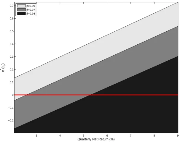
Proposition 6(Liquidity Frontier). ∃!, φ∗ :A×K→Rdefined by:
φ∗(A, K) = [(1−π) (1−θ)−θπ]
λπ [ς
s
t (r(A, K) +λ)−λ]
liquidity constraints (9) bind iffφt< φ∗.
Here, r(A, K) is defined by equation (16). The proposition states that for any (K, A)
selection of the state-space, S, there is a threshold value φ∗ such that if liquidity shocks
fall below that value, the liquidity constraints bind. We call the function φ∗ the liquidity
frontier, as it separates the state space into two regions. Sn is the set of points where the
liquidity constraint binds soφ∗ =∂Sn. The interpretation of the liquidity frontier is simple.
[ςts(r(A, K) +λ)−λ]is the amount of entrepreneurs want to hold atq= 1. Since both types are identical when q = 1, then ςs
t characterizes the demand for equity by both groups. By
propositions1and2, we know thatςs
t (r(A, K) +λ)is the demand for equity stock per unit
of wealth and λ the remaining stock of equity per unit of wealth. The difference between these quantities is the per-unit-of-capital demand for investment.
[(1−π) (1−θ)−θπ]is the degree of enforcement constraint in this economy. As either the fraction of savers,(1−π),or the private benefit of diverting resources,(1−θ),increase, the economy requires more liquid assets to finance a larger amount of down-payment in order to carry out investment efficiently. λπφ is maximal supply of equity. Therefore, the liquidity frontier is the degree of liquidity that allows the largest supply of assets to equal the demand for investment project times the degree of enforcement exactly at the point where q = 1. There are several lessons obtained from this analysis.
Lessons: Proposition 6shows that liquidity shocks have stronger effects as the return to
The proposition is also important because it gives us a good idea of the magnitude that liquidity shocks must have in order to cause a disruption on efficient investment. Since ςs
t ≈ 1, (because it is a marginal propensity to save wealth at a high frequency), then
[ςs
t (r(A, K) +λ)−λ]≈r(A, K).In addition, ifλ≈1,then,
φ∗(A, K)≈(1−θ)
(1−π)
π −
θ
(1−θ)
r(A, K)
By assumption, θ ∈ (0,(1−π)). This implies that θ → 0, φ∗(A, K) will be close to (1−ππ), that the economy requires a very large amount of liquidity to run efficiently. On the other hand, as θ → (1−π), thenφ∗(A, K)will be close to zero implying that the economy does not require liquidity at all. Moreover, we can show that for two values ofθ there is almost-observational equivalence result.
Proposition 7(Observational Equivalence). Let%be a recursive competitive equilibrium defined
for parameters x ≡ (θ,Π,Φ). Then there exists another recursive competitive equilibrium %0 for
parametersx0 ≡ (θ0,Π0,Φ0)which determines the same stochastic process for prices and allocations
as in%iff:
(1−θ0) (1−π)
θ0πλ
ςts(rt+λqt)
qt
−λ
∈[0,1] (21)
for everyqt, rt, ςts ∈ %whenq > 1and φ
∗(A, K;θ0) ∈ [0,1]
forq = 1. If(21)holds then, the new
triplet of parametersΠ0,Φ0 is constructed in the following way: for everyφ ∈ Φ, φ ≥ φ∗(A, K;θ),
assign toΦ0 any valueφ0 ∈(φ∗(A, K;θ0),1). For everyφ < φ∗(A, K;θ),assign the value given by
(21).This procedure defines a map fromΦtoΦ0. Finally,Π0 should be consistent withΠ.
We provide a sketch of the proof here. Condition(21)is obtained by substituting (18) and (19) into (20) at equality. The left hand side of the condition is the solution to aφ0such that for θ0,(20) also holds at equality. If this is the case, then the same q and investment allocations clear out the equity market. Therefore, if the condition required by the proposition holds,φ0 as constructed, will yield the same allocations and prices as the original equilibrium. Since prices are the same, transition functions will be the same and so will the policy functions. If theφ∗(A, K;x0)6∈ [0,1]then liquidity under the new parameters is insufficient. This shows the if part.
By contradiction, assume that the two equilibria are observationally equivalent. If (21)is violated for somes ∈S, then, it is impossible to find a liquidity shock between 0 and 1, such that (20) is solved at equality. For these states,qt >1in the original equilibrium, but qt = 1
in the equilibrium with the alternative parameters.
A final by-product of Proposition6 is its use to compute an estimate of the amount of outside liquidity needed to run the economy efficiently. In order to guarantee efficient in-vestment, an outside source of liquidity must be provided by fraction (φ∗ −φt)λπ of total
capital stock every period. In this case,φ∗should be evaluated atqt= 1at allst.(φ∗−φt)is a
3 4 5 6 7 8 9 −0.2
−0.1 0 0.1 0.2 0.3 0.4 0.5 0.6 0.7
Quarterly Net Return (%)
φ
* (s
t
)
β=0.99
β=0.97
β=0.94
Figure 2: Liquidity Frontier. Numerical Examples.
Figure 2, plots the liquidity frontier as a function of returns r(A, K), for three differ-ent values of β.Simulations show that the marginal propensities to save for values ofθ =
{0.9,0.7,0.5} are close to β = {0.99,975,0.945} respectively. The frontier is increasing in the returns showing that weaker shocks will activate the constraints for higher returns. As the elasticity of intertemporal substitution increases, weaker shocks activate the liquidity constraints.
4
Results
4.1
Calibration
business cycle theory. Following the standard in the RBC literature, technology shocks are modeled such that their natural logarithm follows an AR(1) process. The persistence of the process,ρA,is set to0.95and the standard deviation of the innovations of this process,σA,is
set to0.016. The weight of capital in productionαis set to0.3611. The depreciation of capital is set toλ= 0.974so that annual depreciation is10%.12
The probability of investment opportunities, π, is set to 0.1so that it matches the plant level evidence of Cooper et al. [1999]. That data suggests that around 40% to20% plants augment a considerable part of their physical capital stock. These figures vary according to a given plant’s age. By setting π to0.1, the arrival of investment opportunities is such that close to30%of firms invest by the end of a year.
There is less consensus about parameters governing preferences. The key parameters for determining the allocation between consumption and investment are the time discount factor,β,and the elasticity of intertemporal substitution,σ. The discount factor,β,is set to
0.9762based on a complete markets benchmark, as inCampanale et al.[2010]. For our base scenario, we setσandγto 1 to recover a log-preference structure. We check the robustness of the results by changing these values in an alternative calibration. Nevertheless, the marginal propensities to saveςi andςsare roughly constant over the state-space. Picking a particular combination of these parameters is similar to modifying β an keeping the log-preference structure.13 Campanale et al.[2010] argue in favor of a low value forσbased on experimental
evidence. Angeletos [2007] argues that empirical work based on asset pricing biases the estimate downwards and sets the parameter to 1. For an alternative calibration, we set this parameter to 0.9. The elasticity of intertemporal substitution σ affects the stationary distribution of the capital stock. Under, lower values of this parameter, the capital stock fluctuates around levels for which the return to capital is above25%which seems large. The size of investment over the capital stock is also unreasonably large. In Campanale et al. [2010] this undesirable feature of a low value forσ in our model is corrected by changing the adjustment costs of investment. Adjustment costs are meant to capture some features of lumpy-investment observed in micro-level data. Since random investment opportunities are already capturing that feature, we do not innu such costs. For the alternative scenario, we follow the estimates ofMoskowitz and Vissing-Jørgensen[2002] suggesting a risk aversion parameter of around10for entrepreneurs.
The Frisch-elasticity is determined by the inverse of the parameterν, which is set to 2. This parameter also shifts the curvature of the aggregate production function as a function of the aggregate capital stock. In other words,ν andαare crucial to determine the volatility of the returns to capital as the capital stock fluctuates around the stationary distribution. Volatility is a second order effect: in equilibrium, the distribution of capital will accommo-date so that the average return to capital is consistent with the agent’s marginal propensities to save (equations (24) and (25)). ω¯ is a normalization constant that plays no role in the
11Acemoglu and Guerrieri[2008] have shown that the capital share of aggregate output has been roughly
constant over the last 60 years.
12It is common to find calibrations where annual depreciation is5%. This parameter is crucial in determining
the magnitude of the response of output to liquidity shocks. In particular, this response is greater the larger the depreciation rate. We discuss this aspect later on.
model.
Two sets of parameters remain to be calibrated:θ,the parameter that governs the limited enforcement problem in investment and the parameters related to the liquidity shocks: Φ
and Π. The limited enforcement parameter satisfies 0 ≤ θ < 1− π = 0.9. Thus, there is very large degree of freedom to calibrate θ. Moreover, there is almost an observational equivalence as shown in Proposition7. Therefore, for comparison reasons only, we setθ = 0.15,as this is the value chosen bydel Negro et al.[2010]. The lower and upper bounds ofΦ
are calibrated by setting(φL, φH) = (0.0,0.3). This choice renders an unconditional mean of
liquidity of 0.15 as indel Negro et al.[2010].
The meaning ofθ should not be taken too literally. There are many ways to introduce financial frictions, the simplest of which is the limited enforcement problem presented here. In our view, θ should be understood as a parameter that captures the idea that external financing requires a down-payment to curtail incentives. Neither should 1
θ be understood as
a leverage ratio for the economy. The financial contracts described in the model as such that equity is sold to finance the down-payment. In reality, equity is sold and used as collateral. As described before, this distinction is irrelevant for the model but implies very different leverage ratios.
In the alternative calibration, we choose Φ using as a target a mean risk-free rate of roughly1% and volatility of1.7%which are roughly the values for the U.S. economy.14 We
argued previously that θ and π determine the liquidity frontier. Φ and Π determine how often and how deeply will liquidity shocks enter the liquidity constrained region. Lower values θ andφ (on average) causeq to become increase. These parameters interplay to de-termine the volatility of the price of equity and the stochastic discount factor since they influence the effect on consumption after the entrepreneur switches from one type to an-other (equations (24) and (25)). Based on this consideration, we set(φL, φH) = (0.17,0.25)in
the alternative scenario.
Finally, we describe the calibration strategy for the transition matrixΠ. There are three desirable features that the transition probability Πshould have: (1) That it induces (At, φt)
to be correlated. Bigio [2009] and Kurlat [2009] study the relation between liquidity and aggregate productivity when liquidity is determined by the solution to a problem of asym-metric information. Both papers provide theoretical results in which the relation between productivity and liquidity is positive. (2) ThatAtand φtare independent ofφt−1. In
princi-ple, at least in quarterly frequency, liquidity should not explain aggregate productivity. We relax this assumption in the appendix where we discuss the effects of rare and persistent liquidity crises. (3) At has positive time correlation, as in the RBC-literature. We calibrate
the transition to obtain these properties. In the computerAis discrete. We letΠAbe the
dis-crete approximation to anAR(1) process with typical elementπa0,a = Pr{At+1 =a0|At=a}.
To construct the joint process forAt andφtwe first construct a monotone map fromΦtoA
and denote it by A(φ).This map is simply the order of elements inΦ. LetΠu be a uniform
transition matrix and let ℵ ∈ [0,1]. We fill inΠ by letting its typical element π(a0,φ0)×(a,φ) be
defined in the following way:
Calibration Preferences Technology Aggregate Shocks
β γ σ ν ω α λ π θ ρA µA σA ℵ φL φH
Baseline 0.976 1 1 2 0.9 0.36 0.974 0.1 0.15 0.95 0 0.016 0.95 0 0.3 Alternative 0.976 0.9 10 2 0.9 0.36 0.974 0.1 0.15 0.95 0 0.016 0.95 0.17 0.25
Table 1: Calibration
π(a0,φ0)×(a,φ) ≡ Pr{At+1 =a0, φt+1 =φ0|At =a, φt=φ}
= πa0,a× ℵ ·πA(φ0),a+ (1− ℵ)·Πu
Approximated in this way, Π has all of the 3 properties we desire. The parametrization ℵ
governs the correlation betweenAtandφt.By construction(A, φ)are independent ofφ,but
A follows an AR(1) process. Under this assumption, the model requires 5 parameters to calibrateΠ: (ρA, σA)the standard parameters of theAR(1) process for technology,(φL, φH)
the lower and upper bounds ofΦandℵ the degree of correlation between liquidity shocks and technology shocks.
When we study the asset pricing properties of the model, we find that the standard devi-ation of the risk-free rate approximates better the values found in the data whenℵis close to 1. It is worth noting that when liquidity shocks are endogenous, as inBigio[2009] orKurlat [2009], a high autocorrelation, ℵand (φL, φH)are delivered as outcomes of the model. The
equity premium is higher for a higher values of the correlation. For these reasons we set
ℵ= 0.95.The same risk free rate may be obtained by different combinations ofΦand a new parameterℵ(which we discuss below) but at the expense of affecting its own volatility and the mean of the equity premium.
Alternative Calibration Strategy: An alternative calibration strategy could have followed
from the work of Chari et al. [2007]. These authors estimate an investment wedge for the U.S. economy, by reverse-engineering a wedge in a standard euler equation. The model pre-sented here, delivers a similar wedge for each entrepreneur type. Since the model has two representative entrepreneurs (as well as hand-to-mouth workers), a direct mapping cannot be constructed from the wedges here to the wedges in that paper. An alternative calibra-tion strategy may reverse-engineer the wedges in our paper, and then calibrate the liquidity shocks to deliver similar wedges as found in the data. We leave this task for a more detailed model.
4.2
Qualitative Results
In this section, we describe the main qualitative findings of the model obtained by comput-ing the recursive competitive equilibria.15 These equilibria are computed using a grid size
15Fortran cand Matlab ccodes are available upon request. The codes run in approximately 25 minutes and
of 6 forAandΦ. The grid size for the capital stock is 120. No important changes in the
mo-ments of the data generated by the model are obtained by increasing the grid size. Figure3 plotsq, qi andqRover the state-space. Each panel corresponds to a combination of an
aggre-gate productivity shock and a liquidity shock. The aggreaggre-gate capital state is plotted in the x-axis of each panel. Some plots show a threshold capital level for whichqis above one and equal to1for capital above that level. Those points of the state-space coincide with points where the liquidity frontier is crossed. The figure helps explain how there are two forces in determining qin the model. By comparing the panels in the left from those in the right, we observe how q is lower in states where liquidity is higher. This happens because more liquidity relaxes the enforcement constraint at the aggregate level. To clear out the equity market when liquidity is tighter,qmust increase to deter saving entrepreneurs from invest-ing in projects that don’t satisfy the incentive compatibility constraint. On the other hand, by comparing the upper row with the one on the bottom, we observe the effects of higher ag-gregate productivity. qincreases when productivity is higher. This happens because agents demand more investment at these states since returns are predicted to be higher in the fu-ture. Inside the area below the liquidity frontier, the enforcement constraint is binding at an aggregate level. In these states, q must increase to make investing entrepreneurs invest more, and deter saving entrepreneurs from financing projects externally.
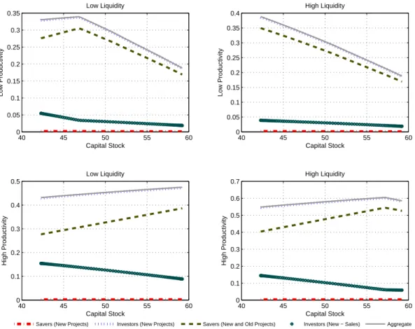
The corresponding plots for aggregate investment are depicted in Figure4. Each panel plots 5 curves. These curves are the aggregate investment, investment in new projects owned by saving and investing entrepreneurs (the aggregate levels of is and ii) and the net change in the equity position of both groups. The plots show that investment is close to being a linear function of capital, but this relation changes when the liquidity frontier is crossed. Why? Notice that there is a kink in aggregate investment when q rises above 1, which corresponds to points inside the liquidity frontier. Outside the liquidity constrained region, the lower the capital stock, the larger the demand to replenish the capital stock (re-turns to equity are higher). Inside the liquidity constrained region, the lower the capital stock, the lower the amount of liquid assets for the same liquidity shock. Because liquidity is lower, investing entrepreneurs have a smaller amount to use as down-payment: invest-ment must be lower. This effect is explained in Section2.5. In addition, there is an important wealth transfer from investing to saving entrepreneurs in the liquidity constrained region. Thus, the overall effect on investment is also influenced by a wealth effect.
in old projects falls as liquidity shocks approach to the liquidity frontier.
Marginal propensities to save are constant and equal toβfor log-utility. Whenσ <1,they satisfy the following characteristics: (1) in the constrained region, investing entrepreneurs have a lower marginal propensity to save which is by a strong governed by a wealth effect; (2) the marginal propensity to save of saving entrepreneurs is decreasing inq and the con-verse is true about investing entrepreneurs. These relations are reverted whenσ > 1. Nev-ertheless, simulations shows that for different choices ofσ,marginal propensities to save are not constant but don’t move very much.
As inHe and Krishnamurthy [2008] andBrunnermeier and Sannikov[2009], this model also highlights the importance of global methods in understanding the interaction between liquidity shocks and the constraints. Is linearizing the model a bad idea? Yes and no. No because, the behavior of inside either region seems to be very linear for our choice of param-eters. This, in fact, is not true for other paramparam-eters. On the other hand, linearization may become problematic. The reason is that it may be highly likely that the liquidity frontier is crossed often because in stochastic environments, the capital stock is often above the desired level of capital. These states necessarily lie in the unconstrained region. Bigio[2009] shows that if illiquidty is caused by asymmetric information, liquidity shocks will fall close to the liquidity frontier. Moreover, in the appendix, we argue that in order to replicate a reasonable risk-free rate, liquidity shocksmustfall close to the liquidity frontier. Because it’s given in an analytical form (at least for log-preferences), the liquidity frontier may be used to asses how close the deterministic steady-states of an approximated model is to the liquidity frontier.
Figure7depicts the marginal uncondition distribution of the capital stock as well as the marginal distribution of conditional on constraints being binding. The next section describes the main quantitative properties of the model.
4.3
Moments
Statistics: Table2 reports the standard RBC moments delivered by the model. The table is
broken into the moments corresponding to the unconditional distribution and conditioned on the event that the economy is in the liquidity constrained region. Whenever they appear, the numbers in parenthesis correspond to the standard deviation corresponding to the av-erage above them. All of the results are computed with respect to the model’s stationary distribution of the aggregate state. The bottom row of the table reports the computed oc-cupation time within the region below the liquidity frontier Sb (the region where liquidity
unconditional volatility of investment over the volatility of output is almost 4 times larger. This relative volatility is much lower within the unconstrained region. This figure is not sur-prising once one considers that workers are not smoothing consumption (on their own will). The fourth and fifth rows describe the average marginal propensities to consume of both en-trepreneurs.16 The seventh column reports the relative size of output within each region.
Output is on average 2.5% lower within the constrained region and 15% larger outside this region. Two things explain this large differences: (1) lower output is associated with a lower capital stock, which in turn, increases returns and the probability of binding constraints. (2) low liquidity is associated with low aggregate productivity shock. Similarly, worked hours are considerably larger within the unconstrained region.
The unconditional correlation between q and investment is negative and close to -95%. This happens because, most of the time, the economy is in the liquidity constrained region and the relation between these two variables is negative in this region (but theoretically undeterminate). The fact that financing constraints can break the relation between q and investment is also found in prior work by Lorenzoni and Walentin [2009]. In our model, the relation between q and investment breaks is explained by Figure 4. The reason is that these correlations are driven by two forces that work in opposite directions: ceteris paribus liquidity shocks reduce these correlations and aggregate productivity shocks increase them. When liquidity shocks hit, the economy is more constrained, so q must rise to clear the market for new equity. This occurs together with a fall in investment. On the other hand, positive productivity shocks drive q as larger returns to equity are expected. q grows to clear out the equity market while investment is larger. The correlation computed under the baseline calibration is considerably lower than in the data. This suggests that the liquidity shocks calibrated here are extremely large, a feature that we openly acknowledge as we want to get as much as we can from the shocks.
Another interesting feature of the model is that it generates right skewness in the station-ary distribution of the capital stock compared to a frictionless economy. The reason is that when the capital stock is lower, the liquidity constraints tend to be tighter. This feature is reflected into less investment than otherwise, which, in turn makes the capital stock recover at a slower pace. On the other hand, the average capital stock is lower in this economy than in a frictionless economy. One way to see this is that under log-preferences, the marginal propensities to save are constant, so all of the effect on investment is through a substitution effect. In the case of saving entrepreneurs, this effect is negative and dominates the increase on investment by investing entrepreneurs.
Results under the alternative calibration: Table 3reports the model’s statistics for the
alter-native calibration. The calibration is such that the model delivers a reasonable risk-free rate, a feature that is discussed in the appendix. The important thing to note here is that the model requires liquidity shocks to be calibrated so that they fall in the region close to the liquid-ity frontier in order to obtain reasonable risk-free rates. Under this alternative calibration, the occupation time of liquidity constraints is 75% which is not very far from the occupa-tion time in the baseline calibraoccupa-tion. In contrast, the magnitude of liquidity shocks is much lower. This reflects itself in the average conditional and unconditional values of q, which