A CAD System for the Automatic Detection
of Clustered Microcalcifications in Digitized
Mammogram Films
Songyang Yu* and Ling Guan
Abstract—Clusters of microcalcifications in mammograms are an important early sign of breast cancer. This paper presents a computer-aided diagnosis (CAD) system for the automatic detec-tion of clustered microcalcificadetec-tions in digitized mammograms. The proposed system consists of two main steps. First, potential microcalcification pixels in the mammograms are segmented out by using mixed features consisting of wavelet features and gray level statistical features, and labeled into potential individual microcalcification objects by their spatial connectivity. Second, individual microcalcifications are detected by using a set of 31 features extracted from the potential individual microcalcification objects. The discriminatory power of these features is analyzed using general regression neural networks via sequential forward and sequential backward selection methods. The classifiers used in these two steps are both multilayer feedforward neural networks. The method is applied to a database of 40 mammograms (Ni-jmegen database) containing 105 clusters of microcalcifications. A free-response operating characteristics (FROC) curve is used to evaluate the performance. Results show that the proposed system gives quite satisfactory detection performance. In particular, a 90% mean true positive detection rate is achieved at the cost of 0.5 false positive per image when mixed features are used in the first step and 15 features selected by the sequential backward selection method are used in the second step. However, we must be cautious when interpreting the results, since the 20 training samples are also used in the testing step.
Index Terms—Computer-aided diagnosis, microcalcification, multilayer feedforward neural network, wavelet transform.
I. INTRODUCTION
T
ODAY, breast cancer is the most frequent form of cancer in women, especially in the western countries. It is also the leading cause of mortality in women each year. The World Health Organization’s International Agency for Research on Cancer in Lyon, France, estimates that more than 150 000 women worldwide die of breast cancer each year [1]. There is clear evidence which shows that early diagnosis and treatment of breast cancer can significantly increase the chance of survival for patients [2]–[5]. The earlier the cancer is detected, the better the chance that a proper treatment can be prescribed. Of all the diagnostic methods currently available for detection of breastManuscript received May 4, 1999; revised December 8, 1999. This work was supported in part by a grant from the Australian Research Council. The Asso-ciate Editor responsible for coordinating the review of this paper and recom-mending its publication was N. Karssemeijer. Asterisk indicates corresponding
author.
*S. Yu and L. Guan are with the School of Electrical and Information Engi-neering, University of Sydney, Sydney NSW 2006, Australia.
Publisher Item Identifier S 0278-0062(00)02298-9.
cancer, mammography is the only reliable and practical method capable of detecting breast cancer at its early stage [6], [7].
With nationwide screening programs in many western countries, the number of mammograms to be analyzed by the radiologists is enormous. However, only a few (approxi-mately 0.5% [8]) cases are actually present with breast cancer. Manual reading, the current examination procedure, is labor intensive, time consuming, and demands great concentration. Furthermore, because of the large number of normal patients in the screening programs, there is a risk that radiologists may miss some subtle abnormalities. The problems associated with the traditional diagnosis procedure prompted medical practi-tioners and scientists in related fields to consider alternative approaches. The rapid advancement of computer technology, pattern recognition, digital image processing, and artificial intelligence has led to a new direction in mammogram analysis and breast cancer diagnosis in recent years. By incorporating the expert knowledge of radiologists, the computer-based systems provide a second opinion in detecting abnormalities and making diagnostic decisions. Such a diagnostic procedure is called computer-aided diagnosis (CAD). A computerized system for such a purpose is called a CAD system. It has been shown that the performance of radiologists can be increased by providing them with the results of a CAD system [9], [10]. Hence, there are strong motivations to develop a CAD system to assist radiologists in reading mammograms.
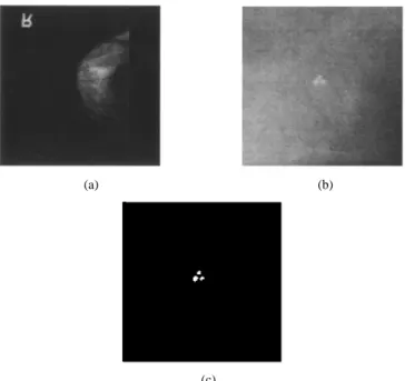
One of the important early symptoms of breast cancer in the mammograms is the appearance of microcalcification clusters, which have a higher X-ray attenuation than the normal breast tissue and appear as a group of small localized granular bright spots in the mammograms. A typical mammogram with clusters of microcalcifications is shown in Fig. 1(a) and the full view of a cluster of microcalcifications in Fig. 1(c).
Computer-aided methods for detecting clustered micro-calcifications have been investigated using many different techniques. Karssemeijer [11]–[13] developed a statistical method for detection of microcalcifications in digital mammo-grams. The method is based on the use of statistical models and the general framework of Bayesian image analysis. Chan
et al. [14]–[16] investigated a computer-based method for the
detection of microcalcification in digital mammograms. The method is based on a difference image technique in which a signal suppressed image is subtracted from a signal enhanced image to remove structured background in the mammogram. Global and local thresholding techniques are then used to extract potential microcalcification signals. Subsequently,
(a) (b)
(c)
Fig. 1. (a) A mammogram from the database. (b) A cluster of microcalcifications in (a). (c) The ground truth image corresponding to the cluster of microcalcifications in (b).
signal extraction criteria are imposed on the potential mi-crocalcifications to distinguish true positives from noise and artifacts. Strickland et al. [17]–[22] developed a method based on undecimated biorthogonal wavelet transforms and optimal subband weighting for detecting and segmenting clustered microcalcifications. Yoshida et al. [23], [24] used decimated wavelet transform and supervised learning for the detection of microcalcifications. Netch [25] proposed a detection scheme for the automatic detection of clustered microcalcifications using multiscale analysis based on the Laplacian-of-Gaussian filter and a mathematical model describing a microcalcification as a bright spot of certain size and contrast. Zheng et al. [26]–[28] proposed a method for the detection of microcalcifications clusters in digitized mammograms using mixed feature-based neural networks. Cheng et al. [29] proposed an approach using fuzzy logic for the detection of microcalcifications.
In this paper, we present the research and development of a CAD system for the automatic detection of the clustered microcalcifications. The proposed system consists of two major steps: segmentation of potential microcalcification pixels and detection of individual microcalcification objects using feature extraction and pattern classification techniques. In the first step, the potential microcalcification pixels are detected and grouped into potential individual microcalcification objects by using mixed features consisting of two wavelet features and two gray level statistical features. The wavelet features are generated by a four-level wavelet decomposition and recon-struction algorithm. The gray level statistical features used in our study are median contrast and normalized gray level value. A multilayer feedforward neural network classifier is then used to generate a likelihood map of potential microcalcification pixels by using the mixed features as inputs. Among these potential individual microcalcification objects there are many false detections due to noise, blood vessels, and dense breast tissue in the mammogram. Therefore, in the second step, these
Fig. 2. Flow chart of our CAD system for the automatic detection of clustered microcalcifications in digitized mammogram films.
potential individual microcalcification objects are classified as true or false individual microcalcification objects using a set of 31 features. The discriminatory power of these features are analyzed and the most discriminatory features are selected by a method using a general regression neural network (GRNN) [30]. A free-response operating characteristics (FROC) curve is used to evaluate the performance of the proposed system. Experiment results show that very satisfactory detection performance has been achieved.
The paper is arranged as follows. In Section II, the mammo-gram database used in our study is introduced. After detailing our method in Sections III and IV, we present the performance of the method on the mammogram database in Section V. Fi-nally, conclusions are drawn in Section VI.
II. MAMMOGRAMDATABASE ANDPREPROCESSING
(a)
(b)
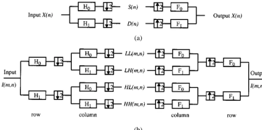
Fig. 3. (a) Filter bank implementation of 1-D wavelet transform. (b) Filter bank implementation of 2-D wavelet transform.
a sampling aperture of 0.05 mm in diameter and 0.1-mm sam-pling distance. The database also comes with a noise equaliza-tion table, which rescales each mammogram image to 256 gray levels. Karssemeijer [13] has shown that the detection result de-pends strongly on this preprocessing step which equalizes the image noise. We applied these scalings to the images as a pre-processing step.
The breast area in this data set only covers about 30%, on average, of each mammogram [13]. Based on this observation, the breast area is first segmented out in order to save processing time and avoid false detections caused by markers and sharp edges near the chest side. Morphological and thresholding tech-niques are used to achieve this purpose. Then further processing is restricted to the breast area.
For the purpose of training the multilayer feedforward neural network, 40 regions of interest (ROI’s) of size 128 128 pixels are randomly selected from the database. Twenty of them con-tain a cluster of true microcalcifications in the center, and the others are chosen from normal areas of the mammogram. There are altogether 174 individual microcalcification objects in the twenty ROI’s which contain a cluster of microcalcification in the center. A ground truth image corresponding to each ROI image was created which contains ones for each pixel consid-ered to be part of a true microcalcification and zeros elsewhere. The ground truth image for the cluster of microcalcifications in Fig. 1(b) is shown in Fig. 1(c).
III. DETECTION OFPOTENTIALMICROCALCIFICATIONPIXELS
The first step of our CAD system is to segment out the pixels that might belong to individual microcalcification objects. This is achieved by using mixed features consisting of wavelet fea-tures and gray level statistical feafea-tures as inputs to a multilayer feedforward neural network to generate a likelihood map of the mammogram.
A. Wavelet Transform
In this subsection we describe the procedure of implementing the one-dimensional (1-D) and two-dimensional (2-D) fast wavelet transform [31]. Interested readers may refer to the following references for wavelet theory [32]–[34].
Wavelets are short basis functions. Unlike sine and cosine which have infinite supports, they drop to zero rapidly. The wavelet transform is implemented by iterations of discrete-time filters. The 1-D wavelet transform is shown in Fig. 3(a). The decomposition part is on the left. It has a lowpass filter and a highpass filter the symbol means downsampling by two—removing the odd-numbered samples. The input signal is filtered by the lowpass filter followed by down-sampling by two to give the low-frequency components. The high-frequency component is created by passing through the highpass filter followed by downsampling by two. Thus, the analysis part yields two half-length outputs and The low-frequency component can be further decomposed into low- and high-frequency component in the same way. The reconstruction part is on the right of Fig. 3(a). It has a lowpass filter and a highpass filter (For orthogonal filter banks is the same as is the same as . For biorthogonal filter banks, they are different). The symbol means upsam-pling by two—inserting zeros between samples. Reconstruction is achieved by first upsampling and and then fil-tered by lowpass filter and highpass filter , respectively. This will get back the original signal if the four filters are chosen correctly. The four filters together are called a perfect re-construction filter bank. In order to achieve perfect reconstruc-tion, the four filters have to obey the following:
(1)
(2)
In order to decompose images, the 1-D wavelet transform is extended to two dimensions. This is achieved by the separable 2-D wavelet transform shown in Fig. 3(b). The decomposition part is on the left. The image is first decomposed row by row using the 1-D wavelet transform, then decomposed column by column, again using the 1-D wavelet transform. This yields four quarter-sized subimages
and The part can be further
B. Wavelet Features and Gray Level Statistical Features
From an image processing point of view, microcalcifi-cations are relatively high-frequency components buried in the background of low-frequency components and very high-frequency noise in the mammograms. Since wavelets are localized in both the space and frequency domains, they have a multiresolution property. This makes it suitable for extracting microcalcifications from low-frequency backgrounds and high-frequency noise. In particular, the wavelet transform decomposes the signal into signal bands of different frequency ranges. It can help to identify useful information relevant to microcalcifications and discard the signal bands which make little contribution to detection.
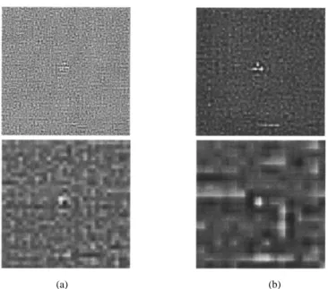
In order to generate the wavelet features, each mammogram image is decomposed up to four levels using the separable 2-D wavelet transform. The wavelet used in this study is Daubechies orthogonal wavelet of length four [33]. The main reason for choosing it is that it needs less computation time comparing to the other wavelets in the Daubechies orthogonal family, while the performance for segmenting microcalcification pixels is comparable to the other ones. It is observed that further decomposition is only sensitive to low-frequency background in the mammograms [35]. Although these subimages may contain useful information for detecting microcalcification pixels, they may not be used readily by a computer for two reasons: 1) because the size of the subimages is smaller than the original image and a subimage in level is one-quarter of the size of a image in level , it is difficult for the computer to find the corresponding pixel in the original image from the subimages and 2) these subimages are sensitive to directions, but microcalcifications are not. Therefore, a reconstruction is performed. We choose to do the reconstruction from each level by setting the transform values of the other levels to zero. This yields four reconstructed images corresponding to levels one to four, respectively. By doing so, we can make sure to preserve all the useful information of microcalcifications and, at the same time, remove the low-frequency background and keep the size of the reconstructed image the same as the original image. The four reconstructed images from levels one to four of the cluster of microcalcifications in Fig. 1(b) are shown in Fig. 4.
By observing these reconstructed images, we note that the reconstructed images from level one are more sensitive to back-ground noise and the reconstructed images from level four are more sensitive to low-frequency background in the mammo-grams. Only the images reconstructed from levels two and three contain meaningful information about the microcalcifications. So we discard the wavelet features from level one and level four and consider adding features from a second source, gray level statistics. Although many such features are available, there are many reasons why only the most effective ones should be se-lected. The most obvious reason is the consideration of compu-tational efficiency. Through experiment, we identified the fol-lowing two effective features: median contrast [36] and normal-ized gray level value (contrast-to-noise ratio) [37] which are de-fined as follows:
medium Window (3)
(a) (b)
Fig. 4. Orthogonal wavelet reconstruction of the mammogram image in Fig. 1(b) from (a) level one to (d) level four, respectively.
mean Window
std Window (4)
where is the pixel value at position Window is an square area centred at position( ), std is the standard deviation of the pixel values in the Window, is the median contrast at position , and is the normalized gray level value at position . Now each pixel in the mammogram is represented by a mixed feature vector of four elements
(5)
where and are the pixel values at position in the reconstructed images from level two and level three, re-spectively, is the median contrast, and is the nor-malized gray level value.
C. Neural Network and Likelihood Map
In order to find the potential microcalcification pixels based on the above mentioned features, a proper classification method must be used. In our study, the classifier chosen is a multilayer feedforward neural network. The main reason for choosing it is because of its nonparametric statistical property. Unlike the classical statistical classification methods, such as the Bayes classifier, no knowledge of the underlying probability distribu-tion is needed by a neural network. It can learn the free pa-rameters (weights and biases) through training by using exam-ples. This makes it suitable to deal with real problems which are nonlinear, nonstationary, and nonGaussian. The neural network classifier is used to generate a likelihood map of each mammo-gram using the mixed features as the input to the classifier. The pixel value in the likelihood map shows the possibility of that pixel being classified as a microcalcification pixel. The larger the value, the more likely it is a microcalcification pixel.
TABLE I
LIST OFFEATURESUSED FOR THEIDENTIFICATION OFINDIVIDUALMICROCALCIFICATIONOBJECTS
of each pixel and two units in the output layer corresponding to microcalcification pixels and normal pixels, respectively. The output unit corresponding to the true microcalcification pixels is then thresholded to segment out the true microcalcification pixels.
The training data set for the above neural network is chosen from the twenty ROI’s with a cluster of microcalcifications in the center. If one microcalcification pixel is picked out from one ROI, a corresponding normal pixel is chosen randomly from the same ROI. This makes the number of microcalcification pixels equal to the number of normal pixels in the training data set. There are totally 1748 microcalcification pixels in the 20 ROI’s. Thus, the size of the training data is 1748 2 4.
After training, the neural network is used to classify the 40 full mammograms in the database. Each pixel in the original mammogram is classified by feeding its mixed feature vector as the input to the network, thus yielding a likelihood map of each mammogram from the feature vector. The likelihood map is then thresholded to get the potential microcalcification pixels. The threshold level is the same for the 40 full mammograms. The criteria for choosing threshold level is to make sure that all the major individual microcalcifications are included in the thresh-olded image. A binary image is generated with zeros for normal pixels and ones for microcalcification pixels after thresholding. Connected pixels in the binary image are considered belonging to potential individual microcalcification objects, which are fur-ther labeled into objects for feature extraction. Single pixels are removed because they are most likely caused by noise. These objects are considered to be potential individual microcalcifica-tion objects.
IV. DETECTION OFINDIVIDUALMICROCALCIFICATION
OBJECTS
In our first step, the potential microcalcification pixels are segmented out using mixed features, and then grouped into po-tential individual microcalcification objects by their spatial
con-nectivity. Because of noise corruption, the mixed features of pixels in dense breast tissue and blood vessels may be sim-ilar to those of the microcalcification pixels. Hence, a large value (near one) may be generated in the likelihood map and the pixels are misclassified as potential microcalcification pixels by the first step. The potential microcalcification objects that are made of these misclassified potential microcalcification pixels are called false individual microcalcification objects. The ex-istence of these false individual microcalcification objects will decrease the performance of our CAD system. In order to elimi-nate these false detections, a second discrimination step is used. In this second step, our CAD system determines whether a po-tential individual microcalcification object segmented out in the first step is a true or a false individual microcalcification object. Karssemeijer’s criteria for counting true positive (TP) and false positive (FP) is adopted. A true cluster is counted to be found if two or more objects in the truth circle are found. A cluster is counted if two or more objects are within the distance of 1 cm. A false positive cluster is counted if none of the objects found in the cluster are inside the truth circle. A feedforward neural network is used as the classifier. In order to generate the FROC curve, the output of the neural network is thresholded at dif-ferent threshold levels. This classification procedure is based on a set of 31 features extracted from these potential individual mi-crocalcification objects. These 31 features are listed in Table I. These features are all calculated from the original image. For calculating the second order histogram related features, a square neighborhood of 10 pixels larger than the potential individual microcalcification object in diameter is used to extract the cooc-currence matrix for each potential individual microcalcification object.
ROI’s with a cluster of microcalcification in the center is used to obtain features for true individual microcalcification objects. To obtain the features for the false individual microcalcification objects caused by noise, blood vessels, and dense breast tissue, the neural network used in the first step is employed to classify the 20 ROI’s extracted from the normal breast area by using its mixed feature vector as input. Then the classification result is thresholded to obtain false individual microcalcification ob-jects. The features of the false microcalcification objects in the 20 normal ROI’s together with the features of the true micro-calcification objects in the other 20 ROI’s, form the training set. There are altogether 338 true/false microcalcification objects in the training data set and 173 of them are true microcalcification objects.
A. SFS and SBS Methods
The performance of a pattern recognition system critically depends on how well the features chosen as the inputs sepa-rate patterns belonging to different classes in the feature space. The ultimate goal of feature selection is to choose a number of features from the extracted feature set that yields minimum classification error. In mathematical terms, the feature selec-tion problem can be expressed in the following way. Let
be a set of possible features providing adequate representation of any pattern belonging to one of classes to be classified. Let be a subset of
features which contain more discriminatory power about than any other subset of features of features in . Let be a measurement of the classification error by using the feature set for classification. Then the feature set must satisfy
(6)
For a pattern recognition problem, the classification error mea-surement is usually the mean square classification error which is defined as
(7)
where is the th pattern to be classified, is the actual output of the classifier, is the desired output, and is the total number of training samples.
The intuitive solution to determine the optimal subset of fea-tures is by exhaustive testing of all the possible combinations, which is equal to . However, even for moderate and , this is a large number and the approach is practically infeasible. Then there exist three more sophisticated feature se-lection methods. The first is by experience which has been used by most researchers in CAD based breast cancer studies [13], [16], [21], [25]. The success of this method relies on the re-searcher’s knowledge of the problem involved. The second is feature transformation, which is implemented in such a way that the transformed features have fewer dimensions than the original features, but have more discriminating power. Principal component analysis [43] is one of the well-known methods in this category. The third is to organize the search method to re-duce the number of feature sets to be evaluated. Woods et al. [44] adopted sequential forward selection and sequential backward
selection methods for the detection of stellate lesion. Dhawan [45], [46] et al. applied the multivariate cluster analysis and ge-netic algorithm based search methods for the analysis of mam-mographic microcalcifications. Kocur [47] et al. used neural network method to select wavelet features for breast cancer di-agnosis, In this paper, we use both the sequential forward selec-tion method and the sequential backward selecselec-tion method for the detection of individual microcalcification objects.
Sequential forward selection is a bottom–up search procedure where one feature at a time is added to the current feature set. At each stage, the feature to be included in the feature set is selected among the remaining available features from which have not been added to the feature set. So the new enlarged feature set yields a minimum classification error comparing to adding any other single feature.
Mathematically, suppose features have been selected to form a feature set . Then select feature from the remaining features to add to so that
for
(8) Then the enlarged feature set is given as
The procedure is initialized by setting =∅.
If we want to find the most discriminatory feature set, the al-gorithm will stop at a point when adding more features to the current feature set increases the classification error. For finding the order of the discriminatory power of all features, the al-gorithm will continue until all the features are added to the feature set. The order in which a feature is added is the rank of the feature’s discriminatory power.
The sequential backward selection is the top down counter-part of the sequential forward selection method. It starts from the complete set of features, At each stage, the feature which shows the least discriminatory power is discarded.
Mathematically, suppose that features have been discarded to form the feature set which has features at this moment. Then the feature is discarded from the remaining
features if
for
(9) Then The procedure is initialized by setting
If we want to find the most discriminatory feature set, the algorithm will stop at a point when further deleting features from the current feature set increases the classification error. For finding the order of the discriminatory power of all features, the algorithm will continue until all the features are deleted from the feature set. The rank of the discriminatory power of a feature is the reverse order in which it is discarded. Hence the first feature discarded has the least discriminatory power, while the last feature discarded has the most discriminatory power.
B. General Regression Neural Networks
Fig. 5. The block diagram of general regression neural network.
needs a large number of iterations to be performed in training to converge to a desired solution, the GRNN needs only a single pass of learning to achieve optimal performance in classifica-tion.
The GRNN is a memory-based feedforward network based on the estimation of probability density function. Originally known as Nadaraya–Watson regression in statistics literature, it is re-discovered by Donald Specht [30]. Let be a vector random variable, be a scalar random variable, and represent the joint probability density function of and . The expected value of given can be computed by
(10)
In practice, the probability density function is usually un-known. Therefore, it must be estimated from sample values of and . The following estimator, also called a kernel func-tion, was proposed by Parzen [48] and adopted here:
(11)
where is the width of the estimating kernel, is the number of samples, and is the dimension of the input vector . Sub-stituting the probability estimator in (11) into (10) gives the de-sired conditional mean of given
(12)
where is defined as
(13)
Fig. 6. The likelihood map of the mammogram in Fig. 1(b).
Fig. 7. The thresholded likelihood map of the mammogram in Fig. 1(b).
The topology of a GRNN is shown in Fig. 5. It consists of four layers: the input layer, the hidden layer, the summation layer, and the output layer. The function of the input layer is simply to pass the input vector variables to all the units in the hidden layer. The hidden layer consists of all the training sam-ples, to . When an unknown pattern is presented, the squared distance between the unknown pattern and the training sample is calculated and passed through the kernel function. The summation layer has two units, A and B. Unit A computes
the summation of multiplied by the
asso-ciated with . The B unit simply computes the summation of The output unit divides A by B to provide the prediction result.
V. IMPLEMENTATION ANDEXPERIMENTALRESULTS
A. Likelihood Map and Feature Extraction
The proposed procedure was tested on the Nijmegen database of 40 mammograms. First, the likelihood map of each mam-mogram is generated by using a multilayer feedforward neural network. The likelihood map is then thresholded to get the po-tential individual microcalcification objects and the 31 features of each potential individual microcalcifications objects are cal-culated. The likelihood map for the mammogram in Fig. 1(b) is shown in Fig. 6 and the thresholded likelihood map is shown in Fig. 7.
B. Feature Analysis Results
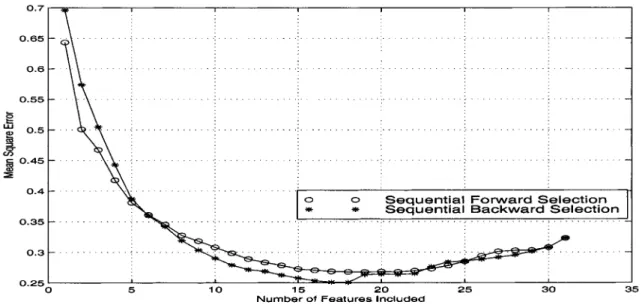
Fig. 8. Feature selection results using SFS and SBS methods.
TABLE II
THEORDER OF THEDISCRIMINATORYPOWER OF THE31 FEATURESOBTAINED BYUSINGSEQUENTIALFORWARDSELECTIONMETHOD
Fig. 8 corresponds to feature order number. For example, for the curve generated by using the SFS method, five features included refer to the top five discriminatory features in Table II, which are feature numbers 11, 5, 22, 1,and 29. From Fig. 8, we can see that when using SFS method, the most discriminatory feature set which gives the minimum mean square error occurs at the point where the top 19 discriminatory features are included and when using SBS method, the most discriminatory feature set which
TABLE III
THEORDER OF THEDISCRIMINATORYPOWER OF THE31 FEATURESOBTAINED BYUSINGSEQUENTIALBACKWARDSELECTIONMETHOD
gives the minimum mean square error occurs at the point where the top 17 features are included.
C. Identification Results Based on Feature Analysis Results
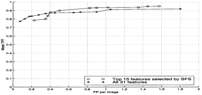
Fig. 9. Comparison of FROC curves obtained by using the top 15 features selected by the SFS method and all 31 features.
Fig. 10. Comparison of FROC curves obtained by using the top 15 features selected by the SBS method and all 31 features.
data set used for feature analysis. Each of the two neural net-works has three layers. The hidden layer has eight units and the output layer has two units, which correspond to true microcal-cification objects and false microcalmicrocal-cification objects, respec-tively. The output unit corresponding to the true microcalcifica-tion objects is thresholded to get individual microcalcificamicrocalcifica-tion objects.
The first neural network used the top 15 features selected by the sequential forward selection method as input. The reason for choosing the top 15 features instead of the top 19 features which gives the minimum mean square classification error is that from Fig. 8, the difference between the mean square clas-sification error using the top 15 features and the top 19 features is so small that it can be ignored. The result is shown in Fig. 9. For a similar reason, the second neural network used the top 15 features selected by the sequential backward method as input. The result is shown in Fig. 10.
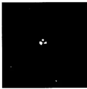
Fig. 11. The final detection result of the mammogram in Fig. 1(b) by using the 15 features selected by SBS.
TABLE IV
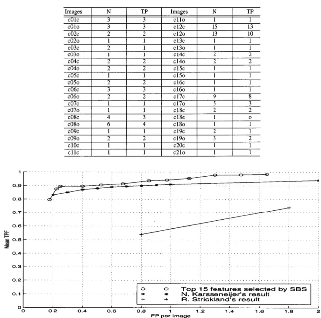
MICROCALCIFICATIONDETECTIONRESULTS AT AFALSEPOSITIVE OF0.5PERIMAGE BYUSING THE15 FEATURESSELECTED BYSBS. THENUMBER OFTRUE
CLUSTERS INEACHMAMMOGRAM IN THEDATABASEISDENOTED BYN. TP IS THETRUEPOSITIVECLUSTERSDETECTED
Fig. 12. Comparison of FROC curves obtained by using the top 15 features selected by the SBS method, N. Karssemeijer’s result and R. Strickland’s result.
31 features. The result using the features selected by the se-quential backward selection method has the best performance. It achieves a 94% mean true positive detection rate at the cost of one false positive per image and a 90% mean true positive detection rate at the cost of 0.5 false positive per image. The final detection result of the mammogram in Fig. 1(b) is shown in Fig. 11. In Table IV, the detection results for each mammo-gram at 0.5 false positive per image are listed. Also plotted in Fig. 12 is the comparison of our results using features se-lected by sequential backward selection with Karssemeijer’s re-sult using the MRF model and IPA scaling with local image fea-ture, namely, local contrast (lc), smoothed local contrast (lcs), and the line/edge feature (lin). It shows that our result, using the features selected by sequential backward selection method, out-performs Karssemeijer’s result. We also plotted the comparison of our best result with Strickland’s result in Fig. 12. It clearly shows the superiority of our method. The experimental results
indicate that using all the 31 features for the detection of indi-vidual microcalcification objects does not give the best perfor-mance, as shown in Figs. 9 and 10. This demonstrates that if a feature does not indicate clearly the difference between the false and true individual microcalcification objects, it will not contribute positively to the classification result.
VI. CONCLUSIONS
step, potential microcalcification pixels are segmented out using mixed features obtained from wavelet transform and gray level statistical analysis and labeled into potential individual microcalcification objects. In the second step, these potential individual microcalcification objects are classified as true or false individual microcalcification objects based on a set of 31 features. The discriminating power of these features is also analyzed using GRNN via SFS and SBS methods. The detected true individual microcalcification objects are then grouped into clusters based on their relative positions. The method is applied to a database of 40 mammograms containing 105 clusters of microcalcifications. Results show that the proposed system gives quite satisfactory detection performance. In particular, a 90% mean true positive detection rate is achieved at the price of 0.5 false positive per image when the 15 features selected by the SBS method are used in the second step. However, caution must be used when interpreting the results since the 20 training samples are included in the testing. Considering that only 20 out of 105 clusters are used in training, the network generalized very satisfactorily. This fact strongly suggests that the selected features are good representations of the microcalcifications and can support robust and effective detection.
ACKNOWLEDGMENT
Images were provided by courtesy of the National Expert and Training Centre for Breast Cancer Screening and the Depart-ment of Radiology at the University of Nijmegen, the Nether-lands.
REFERENCES
[1] R. Gaughan, “New approaches to early detection of breast cancer makes small gains,” Biophotonics Int., pp. 48–53, Sept./Oct. 1998.
[2] S. Shapiro, W. Venet, P. Strax, L. Venet, and R. Roeser, “Ten-to-four-teen-year effect of screening on breast cancer mortality,” JNCL, vol. 69, p. 349, 1982.
[3] R. G. Lester, “The contribution of radiology to the diagnosis, manage-ment, and cure of breast cancer,” Radiology, vol. 151, p. 1, 1984. [4] M. Moskowitz, Benefit and Risk, Breast Cancer Detection:
Mammog-raphy and Other Methods in Breast Imaging, 2nd ed, L. W. Bassel and
R. H. Gold, Eds. New York: Grune and Stratton, 1987.
[5] R. A. Smith, “Epidemiology of breast cancer categorical course in physics,” Tech. Aspects Breast Imaging, Radiol. Soc. N. Amer., pp. 21–33, 1993.
[6] H. C. Zuckerman, The Role of Mammogram in the Diagnosis, Breast
Cancer in Breast Cancer, Diagnosis and Treatment, I. M. Ariel and J. B.
Cleary, Eds. New York: McGraw-Hill, 1987, pp. 152–172.
[7] R. McLelland, “Screening for breast cancer: Opportunity, Status and Challenges,” in Recent Results in Cancer Research, S. Brüner and B. Langfeldt, Eds. Berlin, Germany: Springer-Verlag, 1990, pp. 29–38. [8] M. L. Giger, “Current issues in CAD mammography,” in Digital
Mammography ’96, Proc. 3rd Int. Workshop on Digital Mammography,
Chicago, IL, June 1996, pp. 53–59.
[9] H. P. Chan, K. Doi, C. J. Vyborny, R. A. Schmidt, C. E. Metz, K. L. Lam, T. Ogura, Y. Wu, and H. MacMahon, “Improvement in radiologist’s de-tection of clustered microcalcifications on mammograms,” Investigative
Radiol., vol. 25, pp. 1102–110, 1990.
[10] S. Astley, I. Hutt, and S. Adamson et al., “Automation in mammography: Computer vision and human perception,” Int. J. Pattern Recognit.
Arti-ficial Intell., vol. 7, no. 6, pp. 1313–1338, 1993.
[11] N. Karssemeijer, “A stochastic model for automated detection of calci-fications in digital mammograms,” in Proc. 12th Int. Conf. Information
Processing Medical Imaging, Wye, U.K., July 1991, pp. 227–238.
[12] , “Recognition of clustered microcalcifications using a random field model, biomedical image processing and biomedical visualization,” in
SPIE Proc., vol. 1905, San Jose, CA, 1993, pp. 776–786.
[13] , “Adaptive noise equalization and recognition of microcalcifica-tion clusters in mammograms,” Int. J. Pattern Recognit. Artificial Intell., vol. 7, no. 6, pp. 1357–1376, 1993.
[14] H. P. Chan, K. Doi, S. Galhotra, C. J. Vyborny, H. MacMahon, and P. M. Jokich, “Image feature analysis and computer-aided diagnosis in digital radiography, 1. Automatic detection of microcalcifications in mammog-raphy,” Med. Phys., vol. 14, no. 4, pp. 538–548, July/Aug. 1987. [15] H. P. Chan, K. Doi, C. J. Vyborny, K. L. Lam, and R. A. Schmidt,
“Com-puter-aided detection of microcalcifications in mammograms method-ology and preliminary clinical study,” Investigative Radiol., vol. 23, pp. 664–671, 1988.
[16] H. P. Chan, K. Doi, C. J. Vyborny, R. A. Schmidt, C. Metz, K. L. Lam, T. Ogura, Y. Wu, and H. Maxmahon, “Improvement in radiologists’ detection of clustered microcalcifications on mammogram: The poten-tial of computer-aided diagnosis,” Investigative Radiol., vol. 25, pp. 1102–1110, 1990.
[17] R. N. Strickland and H. I. Hahn, “Wavelet transforms for detecting microcalcifications in mammography,” in Proc. Int. Conf. Image
Processing, Austin, TX, 1994, pp. 402–406.
[18] , “Detection of microcalcifications using wavelets,” in Digital
Mammography’94, Proc. 2nd Int. Workshop Digital Mammography,
York, U.K., July 12, 1994, pp. 79–88.
[19] , “Wavelet transform matched filters for the detection and classi-fication of microcalciclassi-fications in mammography,” in Proc. IEEE Int.
Conf. Image Processing, Washington, DC, Oct. 1995, pp. 422–425.
[20] R. N. Strickland, H. I. Hahn, and L. J. Baig, “Wavelet methods for com-bining CAD with enhancement of mammograms,” in Medical Imaging
1996: Image Processing, SPIE Proc., vol. 2710, 1996, pp. 888–903.
[21] R. N. Strickland and H. I. Hahn, “Wavelet transform for detecting mi-crocalcifications in mammograms,” IEEE Trans. Med. Imag., vol. 15, pp. 218–229, Apr. 1996.
[22] , “Wavelet transform methods for objects detection and recovery,”
IEEE Trans. Image Processing, vol. 6, pp. 724–735, May 1997.
[23] H. Yoshida, K. Doi, and R. M. Nishikawa, “Automated detection of clustered microcalcifications,” in Digital Mammograms Using Wavelet
Transform Techniques, Medical Imaging 1994: Image Processing, Proc. SPIE, vol. 2167, Newport Beach, CA, Feb. 1994, pp. 868–886.
[24] H. Yoshida, W. Zhang, W. Cai, K. Doi, R. M. Nishikawa, and M. L. Giger, “Optimizing wavelet transform based on supervised learning for detection of microcalcifications in digital mammograms,” in Proc. IEEE
Int. Conf. Image Processing, vol. 3, Washington, DC, Oct. 1995, pp.
152–155.
[25] T. Netsch, “A scale-space approach for the detection of clustered micro-calcifications in digital mammograms,” in Digital Mammography 96,
Proc. 3rd Int. Workshop Digital Mammography, Chicago, IL, June 1996,
pp. 301–306.
[26] B. Zheng, W. Qian, and L. P. Clarke, “Artificial neural network for pat-tern recognition in mammography,” in Proc. World Congress Neural
Networks, San Diego, CA, June 1994, pp. I-57–I-62.
[27] , “Multistage neural network for pattern recognition in mammog-raphy,” in Proc. IEEE World Conf. Computational Intelligence, Orlando, FL, July 1994, pp. 3437–3441.
[28] , “Digital mammography: Mixed feature neural network with spec-tral entropy decision for detection of microcalcifications,” IEEE Trans.
Med. Imag., vol. 15, pp. 589–597, Oct. 1996.
[29] H. Cheng, Y. M. Lui, and R. I. Feiimanis, “A novel approach to micro-calcification detection using fuzzy logic techniques,” IEEE Trans. Med.
Imag., vol. 17, pp. 442–450, June 1998.
[30] D. F. Specht, “A general regression neural network,” IEEE Trans. Neural
Networks, vol. 2, pp. 568–576, Nov. 1991.
[31] G. Strang and T. Nguyen, Wavelets and Filter Banks. Cambridge, MA: Wellesley-Cambridge , 1996.
[32] O. Rioul and M. Vetterli, “Wavelets and signal processing,” IEEE Signal
Processing Mag., pp. 14–38, Oct. 1991.
[33] I. Daubechies, Ten Lectures on Wavelets, Society for Industrial and
Ap-plied Mathematics. Montpelier, VT: Capitol City Press, 1992. [34] M. V. Wickerhauser, Adapted Wavelet Analysis from Theory to
Soft-ware. Piscataway, NJ: IEEE Press, 1993.
[35] S. Yu, S. Brown, Y. Xue, and L. Guan, “Enhancement and identification of microcalcifications in mammogram images using wavelets,” in IEEE
SMC Conf. Proc., 1996, pp. 1166–1171.
[36] H. Kong, “Self-organizing tree map and its applications in digital image processing,” Ph.D. thesis, Dept. Elect. Eng., Univ. of Sydney, Sydney, Australia, 1998.
[38] J. A. Freeman and D. M. Skapura, Neural Networks Algorithms,
Applications, and Programming, Techniques. Reading, MA: Ad-dison-Wesley, 1991.
[39] L. Shen, R. M. Rangayyan, and J. E. Leo Desautels, “Shape analysis of mammographic calcifications,” in Proc. Fifth Annu. IEEE Symp.
Com-puter-Based Medical Systems, June 1992, pp. 123–128.
[40] R. C. Gonzalez and R. E. Woods, Digital Image Processing. Reading, MA: Addison-Wesley, 1993.
[41] R. M. Haralick, K. Shanmugam, and I. Dinstein, “Textures features for image classification,” IEEE Trans. Syst., Man, Cybern., vol. SMC-3, pp. 610–621, Nov. 1973.
[42] J. Kittler, Feature Selection Algorithm, Pattern Recognition and Signal
Processing, C. H. Chen, Ed. Alphen aan den Rijn, Germany: Sijthoff & Noordhoof, 1978, pp. 41–60.
[43] S. Haykin, Neural Networks: A Comprehensive Founda-tion. Englewood Cliffs, NJ: Prentice-Hall, 1994.
[44] K. S. Woods and K. W. Bowyer, “Computer detection of stellate lesions,” in Digital Mammography ’94, Proc. 2nd Int. Workshop Digital
Mam-mography. York, U.K., July 12, 1994, pp. 221–229.
[45] A. P. Dhawan, Y. Chitre, C. Kaiser-Bonasso, and M. Moskowitz, “Anal-ysis of mammographic microcalcifications using gray-level image struc-ture feastruc-tures,” IEEE Trans. Med. Imag., vol. 15, pp. 246–259, June 1996. [46] C. C. Peck, A. P. Dhawan, and C. M. Meyer, “Use of genetic algorithms for input selection for feedforward neural networks,” in Proc. IEEE Int.
Conf. Neural Networks, vol. II, 1993, pp. 1115–1122.
[47] C. M. Kocur, S. K. Rogers, L. R. Myers, T. Burns, M. Kabrisky, J. W. Hoffmeister, K. W. Bauer, and J. M. Steppe, “Using neural networks to select wavelet features for breast cancer diagnosis,” IEEE Trans. Eng.
Med. Biol. , pp. 95–102, May/June 1996.
[48] E. Parzen, “On estimation of a probability density function and mode,”
Ann. Math. Statist., vol. 33, pp. 1065–1076, 1962.