Designing ecological and biodiversity sampling strategies

(1)

Designing ecological and biodiversity

sampling strategies

(2)

(3)

Designing

e

cological and

biodiversity sampling strategies

(4)

LIMITED CIRCULATION

Correct citation: Coe, R. 2008. Designing ecological and biodiversity sampling strategies. Working Paper no. 66

Titles in the Working Paper Series aim to disseminate interim results on agroforestry research and practices and stimulate feedback from the scientific community. Other publication series from the World Agroforestry Centre include: Agroforestry Perspectives, Technical Manuals and Occasional Papers.

Published by the World Agroforestry Centre United Nations Avenue

PO Box 30677, GPO 00100 Nairobi, Kenya

Tel: +254(0)20 7224000, via USA +1 650 833 6645 Fax: +254(0)20 7224001, via USA +1 650 833 6646 Email: icraf@cgiar.org

Internet: www.worldagroforestry.org

This paper forms part of Chapter 2 of A Handbook Of Tropical Soil Biology: Sampling and

Characterization of Below-ground Biodiversity, edited by Fatima M. Moreira, E. Jeroen Huising and David E. Bignell (2008, Earthscan, London, ISBN 978-1-84407-593-5). This paper is published separately with permission of Earthscan.

The views expressed in this publication are those of the author and not necessarily those of the World Agroforestry Centre.

(5)

About the authors

Richard CCoe,

Head of the ICRAF-ILRI Research Methods Group,

World Agroforestry Centre (ICRAF),

PO Box 30677, Nairobi, Kenya.

(6)

Abstract

Empirical studies of patterns in biodiversity and other ecological phenomena require

field measurements. While finding a method of measurement at a predetermined site

can be challenging, the locations at which samples are to be taken also have to be

chosen. Despite many years of empirical field research in ecology, many studies seem

to adopt designs which are poorly suited to their purpose. This paper discusses some

of the key issues regarding sampling design in such studies.

Objectives of the study should drive all aspects of design, hence clear and

unambiguous objectives are a prerequisite to good design. These objectives must

include testing hypotheses. Most practical designs are hierarchical. Questions of

replication and sample size can only be addressed once the hierarchy is understood,

and the scales at which different objectives will be met are identified. Stratification is

a key tool in making the design efficient for testing hypotheses. At any level in the

hierarchy there are options of using either systematic or random sampling, with

advantages and disadvantages of both. High levels of unexplained variation are

typical in many ecological studies, and may mean no useful results are obtained. The

(7)

Acknowledgements

The ideas in this paper were prompted by discussions with Jeroen Huising and other

members of the CSM-BGBD project team. I also acknowledge UNEP-GEF, which

provided funds enable us attend project meetings, Simoneta Negrete Yankelevich for

very helpful comments on the initial draft, and Earthscan for granting me permission

(8)

1. Introduction

The study and understanding of biodiversity has become increasingly important over

the past few years, with much data being collected, interpreted and discussed. Yet,

there is no single operational definition of the term ‘biodiversity’ (Magurran 1996,

Yankelevich 2008). This is not uncommon in ecology and other areas of research.

Often vague and complex concepts (such as sustainability or poverty) are discussed

without definition. Scientists take implicit definitions, selecting practical indicators

which, they argue, describe the aspects of the phenomenon that they interested in.

This weak link in scientific method is at the heart of much debate. In this paper, I do

not attempt to resolve the issue. Instead, I assume that the definition and indicators

taken in any study have some validity and focus on problems of designing data

collection for any defined indicator.

Empirical studies of patterns in biodiversity and other ecological phenomena require

field measurements. This paper discusses some of the key issues regarding the choice

of measurement methods and selection of sites for sampling. It was motivated by a

large study of below ground biodiversity (Conservation and Sustainable Management

of Below Ground Biodiversity (CSM-BGBD), http://www.bgbd.net/), but the ideas

are useful in other application areas.

As will be discussed in Section 3, the problem of choosing the location of

measurement points is one that occurs at different scales. At one scale, we have to

choose where the whole study will be located. At another, we need to choose where at

a measurement site (e.g. a 20 x 20 m quadrant) 4 cores for soil chemical analysis will

be taken. Somewhere between the two is the problem of choosing the measurement

sites. While the argument gets a little more complex than this, the problem can be

visualised as choosing the number and location of points in the study landscape at

which the measurement protocols will be implemented.

There is a long tradition of sampling in field ecology, and hence much experience has

been gathered in this field. In addition, there is a well established theory of sampling

for any application area (Cochran, 1977). There are numerous texts describing both

theory and application (e.g. Southwood and Henderson, 2000; Gregoire and

Valentine, 2007). So why is another discussion of sampling in ecology needed?

Despite the knowledge and experience, in any project there will be intense — and

sometimes divisive — discussion of the sampling strategy. There are a number of

(10)

1. Application of the theory or methods successfully used in other studies interacts with

the practical constraints of the new study being designed. For example, it may not be

feasible to take as many samples as you would like due to limited time and cost or

restricted access to ideal sampling locations.

2. Application of sampling theory may require information that is unknown until the

data are collected. For example, the sample size required depends on the variation

between samples. If similar data has not been collected previously then this variation

is not known at the start of the study.

3. There may be limits to the theory. More importantly, there are common

misunderstandings of some of the basic principles, such as the why random sampling

works or what is meant by replication.

4. The objectives of the study drive the design. However, these may not be fully

developed, or there may be multiple objectives that require different approaches to

sampling.

5. Scientists take differing philosophical stands on approaches to sampling, with a

dichotomy between those who aim to ‘see what is there, then seek to understand it’

and those who ‘start with a hypothesis and seek to test it’.

In this paper, I describe some of the options for sampling and the advantages of

(11)

2. Study objectives and sampling basics

Most authors on research study design emphasise the point that the design is

determined by the objectives. Kenkel et al (1989) explain this clearly in the context of

ecological sampling. Many of the debates about appropriate sampling methods turn

out to be due to differences of opinion as to the exact objectives of the study. Ford

(2000) comprehensively discussed research objectives and approaches in ecology.

Simple random sampling (SRS) is the starting point for discussions on sampling. If

the objective is to estimate a population mean (such as the mean biomass of beetles

per m2 within the study area, or the mean number of fungi species within 1 cm3), then

SRS has important properties. The mean of the sample is an unbiased estimate of the

population mean, and its standard error can be estimated without making any

assumptions about the variation within the population (technically, a design-based

estimate of sampling error is available). It is also intuitively appealing. Standard

theory then shows how the precision of the estimate can be controlled by choice of

sample size and the precision increased (for a fixed sample size) by stratification. A

useful alternative to SRS is systematic sampling on a grid, discussed in Section 6.

But few ecological surveys have the limited objective of estimating such a population

mean. An example of an objective that requires a very different approach to sampling

is that of inventory. If the aim is to identify all the species of a given group occurring

in the study area, then SRS is not appropriate. Think of a rare niche in the landscape

(e.g. the bank of a pond which falls on the boundary between forest and field). There

will be a tiny proportion of the whole study area occupied by such niches, so if we are

trying to estimate the mean beetle biomass, it does not matter if such locations are

omitted from the sample. But those rare niches may well be home to species found

nowhere else in the area and, hence, should be included when the objective is

inventory.

Many studies of biodiversity aim to understand patterns of species occurrence. One

approach to sampling is to collect data by SRS or a grid sample, describe the patterns

(for example by clustering and ordination) and then to explain them (for example,

finding correlations with environmental variables). The alternative is to formulate

some hypotheses predicting and explaining patterns in biodiversity, then design a

study specifically aiming at testing the hypotheses.

Proponents of the first approach may claim that they do not want to be ‘biased’ by

(12)

starting out with a limited objective. They would rather ‘keep an open mind’ and see

what they can see. Of course important discoveries in ecology have been made by

chance rather than through planned studies, and every scientist should permanently be

open to the possibility of unanticipated observations, and truly novel explanations.

But there are at least four reasons for trying to design a study with specific objectives,

including testable hypotheses.

1. Without a clear hypothesis, it is impossible to say whether finding no pattern is the

result of none existing or of inadequate (insufficient or inefficient) sampling. There is

no basis for evaluating the success of such a study.

2. Those serendipitous discoveries that might be made usually have the nature of

hypothesis formulation — observations which suggest explanations. Carefully

planned studies are needed to test the explanations.

3. The proponents of the ‘no hypothesis’ approach actually do have some hypotheses,

but these are implicit. For example, without some notion of environmental factors that

might be controlling biodiversity, it is impossible to choose which of an almost

infinite number of such factors should be measured at sample locations. If the implicit

hypotheses are made explicit, study designs can be improved.

4. If we have specific hypotheses, it is often possible to improve the study design,

making the study more efficient.

The last point is behind much of what follows in this paper. Suppose the hypothesis is

that an indicator of below ground biodiversity (BGBD) in agricultural plots is

determined by the level of disturbance (D) and the level of soil organic matter (SOM).

If we collect data by SRS or grid sampling, then it is likely that:

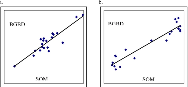
a) Most sample locations will have values of D and SOM around the average,

with relatively few points with very high or low values. But when seeking

to understand the relationship between BGBD and SOM or D, it is the

more extreme points that provide most of the information (Figure 1).

Stratification — dividing the population or study area into sub-populations

and deliberately sampling each — can be used to increase the number of

points with more extreme SOM and improve the estimate of the

(13)

b) SOM and D may well be correlated, for example with plots with high D

typically having low SOM. In such a case, it is hard or impossible to

disentangle the effects of the two variables. However, the study could be

designed to deliberately include some samples with high D and high SOM

as well as others with low D and low SOM. Then the effects of both

variables, and their combined effect, can be estimated.

In practice, it may not be possible or useful to produce a single index of BGBD or D,

as plotted in Figure 1, and relationships may be more complex than straight lines but

the same principles of design apply.

a. b.

BGBD BGBD

SOM SOM

Figure 1. Designs for estimating the relationship between BGBD and SOM.

(a) Simple random or grid sampling will probably give most SOM values near the

average, and a poor estimate of the line. (b) Deliberately including samples more

extreme SOM values through stratification increases the precision of the estimate of

the line at no extra cost.

Another example of a hypothesis implicit in many studies is that of the spatial scale at

which interesting patterns occur. By choosing the distance between sample locations

and the overall size of the study area, the scientist is making choices and assumptions

about the important scales to study. If these are made explicitly, then they are open to

debate, with a likely improvement in the study design.

The overall objective of a project may be to test the hypothesis that increasing land

use intensity changes an indicator of below ground biodiversity, as in the

CSM-BGBD project. This is a rather general statement, but can still be helpful in focusing

(14)

certain way to determine the effect of changing something is to change it, and that is

the basis of an experimental approach. However, this is often not feasible. If we have

to use an observational study design, rather than experimental, then the ideal would be

a longitudinal study, in which plots are monitored over time to see whether changes in

BGBD are correlated with changes in land use.

Generally, this is also not feasible in a project of a short and fixed duration, as the

time over which monitoring may be needed is unknown. Hence the study, like many

others, will have to use a cross-sectional approach, looking at a range of land uses at

one time point. The hope is that correlations between land use intensity and current

BGBD do reflect some causal connections and give indications of what would happen

to BGBD if land use changes take place in the future. Though the validity of this

approach can be questioned, it is often the only option available. Discussions in this

paper therefore only consider alternative sampling schemes for collecting

cross-sectional data.

Note that if historical land use data is available, then it is potentially possible to

examine the effect of different histories of land use. For example, comparing land use

A following B with A following C. However, if A always follows B, it is not possible

to determine whether differences between A and D are a property of A, of B, or of the

sequence B followed by A.

3. Practical approaches

Designing a successful, practical sampling scheme is an art1. It requires deep

understanding of the scientific basis of the research and of the properties of alternative

methods. But these need to be blended with the practical constraints imposed by cost,

the time and expertise available. There may well be additional constraints such as

limited access to desirable sample locations, or the need to rapidly transport samples

from the field to the lab. Details of how these practical and theoretical sides can be

merged will be different for every study and give each investigation its own unique

aspects. However, it is possible to outline steps in the process that can be followed in

any study.

(15)

Step 1: Define objectives

As outlined in Section 2, the objectives determine all aspects of the design. Hence

they must be clearly and precisely determined at the start. Objectives of a research

study must include testing of precisely stated hypotheses. A study may well have

additional objectives, such as compiling a species inventory or estimating parameters

that characterise the study area, that are not usefully stated as hypotheses.

Write down the objectives, so that it is easy to share them with others for suggestions

on how to improve them. Get comments and suggestions from as many other

scientists as you can. These could be scientists working on similar topics but in other

locations, those who have worked in the same location or those with experience in the

methods you plan to use.

One tool to help refine objectives is the simulated presentation of results. Imagine you

have completed the study and obtained results. What tables and graphs would you like

to be able to present to meet your objectives and provide evidence for your

hypotheses? Write these down, with realistic numbers and patterns.— Figure 1 is a

simple example. Then check carefully (a) that those results really would meet the

objectives and, in particular, allow you to reach conclusions about the hypotheses, and

(b) that the sample design imagined could give those results.

Step 2: Review other studies

Look at reports from other related studies. While each study has some unique aspects,

you can learn from earlier studies. Try to understand which aspects of the methods

used appeared successful, and which ones seemed to limit the efficiency or quality of

results. Note in particular sample sizes used and the variability in results.

Step 3: Assemble background data

Assemble background information that will be needed to design sampling details.

These include topological maps (for example, to stratify by altitude or understand

access problems), remote sensing images (to map ground cover), land use maps (to

identify the main land uses to include in the study), meteorological data (to help

decide on suitable seasons for field sampling).

Step 4: Produce a design

Produce a tentative design using a combination of general principles, your own

(16)

do not know much about, but make a realistic suggestion. Write the design down in as

much detail as possible.

Step 5: Review the design

Give the design to other scientists to review and make comments. Again, these may

be people who have worked on similar topics, used similar methods, worked in the

location or are generally perceptive. Include a statistician with experience in

ecological research. A statistician is likely to see aspects of the problem that

ecologists might be missed.

S

tep

6: Pilot

Try out the approach. A pilot investigation is a chance to evaluate the practicality of

the sampling scheme. It also allows testing and refinement of measurement protocols,

data handling procedures, etc. It also allows estimation of the time needed to find,

collect and process samples. If it is possible to process some measurements to the

point of statistical analysis, the pilot also gives an indication of variability, which can

then be used to decide final sample sizes.

Step 7: Iterate

At any step, expect to go back to an earlier one and try again. In particular, revise

objectives in the light of new information and insights. A common mistake is to get

information which suggests the objectives are unobtainable but to carry on anyway.

4. Hierarchy, replication and sample size

Most study designs are hierarchical and the sampling problem is not simply one of

selecting measurement locations within a study area. The CSM-BGBD project

provides a good example. It involves several countries. Within each country one or

more benchmark locations were selected. In each benchmark, one or more study areas

(labelled ‘windows’) were selected. Within each study area, about 100 sample

locations were selected. Measurements are taken at each sample location The

measurement protocol defines further layers in the hierarchy, such as 4 cores being

taken for soil characterisation, and subsamples of the cores subject to chemical

analysis.

At each layer in the hierarchy, the basic sampling questions recur: How many units

(17)

based on scientific grounds. Selection of countries may be based on politics or the

interests of funders and researchers leading the project. But at some level, selection

should be based on the objectives of the study and application of some principles.

The first is the sampling theory idea of a ‘population’ to be sampled. The terminology

is confusing, as this has nothing to do with a biological population. The notion is one

of knowing what your results will refer to. As an example, we could study below

ground biodiversity on farms around the forest boundary of Mt Kenya. That would

require a sample of farms from that location. If we wanted results that apply to the

forest boundaries on mountains in East Africa generally, then we need samples from

some of the other mountains as well. Without that, we can only make statements

about Mt Kenya on the basis of the data, with extrapolation to other locations

dependant on other information or assumptions. The implication for sampling is that

the overall area about which we want to makes inferences (the ‘population’) needs to

be delineated before a sampling scheme can be determined.

The second idea is that of replication, which concerns consistency of patterns and

relationships. The aim of research is to find some patterns, such as patterns of below

ground diversity related to land use. Patterns of interest are those which are consistent

across a number of cases, as it is only these that can be used for prediction and may

reflect some underlying rules or processes. Hence we need repeated observations to

determine whether patterns are indeed consistent.

Suppose we have 10 samples taken from a forest and 10 from nearby cultivated fields,

and the forest plots consistently have higher BGBD. What can we conclude? If the

samples were selected appropriately, we can conclude (to a known degree of

uncertainty assessed by the statistical analysis) that the forest is more diverse than the

fields. But strictly speaking, we can only conclude that that particular forest is more

diverse, not forests in general. If we seek a more general conclusion, then we should

look for consistency across several forests.

Within a hierarchical study design, higher level units such as benchmark sites may

provide one level of replication and consistent patterns across benchmark sites

probably represent some widely applicable ‘rule’. But within benchmark, sites we

would make stronger conclusions if we ensured that several, rather than a single,

forest (or other land use element), are sampled. Multiple samples from the same forest

may not serve the same purpose, representing ‘pseudo-replicates’. The extent to

which repeated samples within one forest serve the same purpose, or can be

interpreted the same way as samples from different forests depends on properties of

the data and not of the design. The safe approach is to ensure valid replication and

(18)

a. b. c. d.

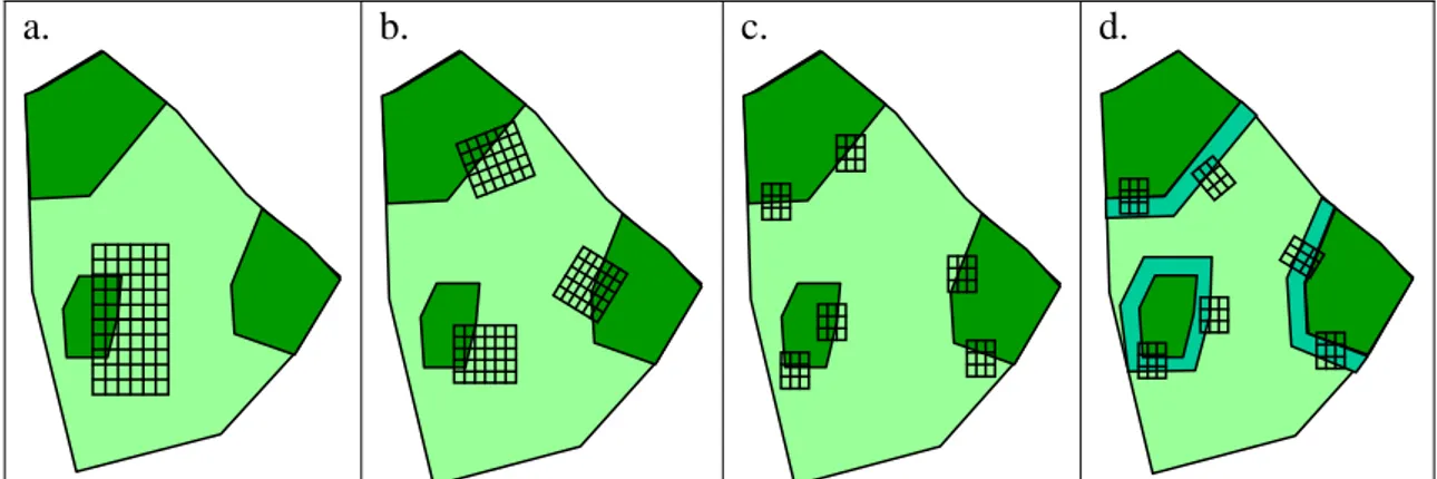
Figure 2: Four approaches to using grid sampling in a landscape with two land uses,

forest and agriculture. (a) A single grid that includes 1 forest patch, (b) 3 grids that

sample 3 different forest patches, (c) increasing the replication, and (d) recognising

the boundaries as another category.

Some of the implications of these ideas for grid sampling (Section 6) are illustrated

for a simplified example in Figure 2. The aim is to sample a landscape with two land

uses, labelled ‘forest’ and ‘agriculture’, in order to examine differences in BGBD. In

Figure 2a, a single large grid has been laid down in such a way as to include both land

uses. The grid is a single ‘window’ with 77 sampling locations (intersections) defined.

In Figure 2b, three smaller windows are used in order to sample three different forest

patches, rather than one only. The replication can be further increased, and more of

the whole study area observed, by using more, smaller windows (Figure 2c).

One criticism of this third design is that all the sample locations in agricultural land

fall close to a forest boundary, and may not be considered representative of the land

use. A response to this is to define a new category of ‘forest boundary’ and ensure

that windows sample all three (Figure 2d). Notice that it is not necessary to have all

land uses sampled in each window. If this process of reducing the size of windows

while increasing their number is continued, then eventually we loose the possible

advantages of grid sampling (Section 6) and end up with a design that looks like a

random sample of individual locations.

‘Scale’ is a confusing and controversial idea in ecology (Peterson and Parker 1998),

but it is clear that the scale at which we anticipate (or hypothesise) patterns

determines the level in the hierarchy at which replication is required. For example, the

hypothesis may be ‘BGBD in agricultural plots decreases with increasing distance

from the forest edge’. This can be investigated with plots (sample locations) at a range

(19)

A different hypothesis is ‘BGBD in agricultural plots decreases with decreasing forest

cover in the landscape’. Here we need to define what is meant by ‘in the landscape’

— that is, the spatial scale at which forest cover is assessed. Suppose that was defined

as areas of 1km2. Then the hypothesis needs a sample of 1km2 units with varying

levels of forest cover. Replication now dictates the need for several such units at each

level of forest cover. To assess the BGBD within such a 1km2 unit, will require

further sampling, with definition of some sample locations within each unit. The

replication at the within-unit level is important for determining the precision with

which the BGBD for each unit is measured, but it is not relevant to affirming the

consistency of pattern across 1km2 units, needed to examine the hypothesis.

In other areas of ecology, landscape factors (e.g. forest fragmentation) are found to

affect processes, so objectives of a BGBD project may include ‘landscape analyses’.

The two examples in the previous paragraph are both examples of analyses that use

landscape factors, yet are based on data from different levels in the hierarchy — one

using plot-level data and the other data from 1km2 units. The message is clear:

‘landscape level’ is not well defined and aiming to do a ‘landscape level analysis’

does not tell you the sampling design needed.

Once we know what is to be replicated, standard methods are available to help select

sample size and so is software to implement them. The methods require knowledge of

two things: the magnitude of difference (for example, differences in BGBD between

two land uses) that it is important to detect, and the variability between replicates of

the same land use. It is clear why the sample size decision depends on these, but it is

usually rather hard to specify them. When research is directed at measuring economic

responses to management decisions (e.g. crop response to fertilizer), then it is feasible

to specify a minimum response that it is important to detect. However, when the

research aims to detect and understand processes, it is often impossible to specify a

size that is important.

A rough estimate of variance between replicates can often be obtained from previous

studies, but how relevant these will be in new environments may be unknown.

Another complication arises from the multivariate responses of interest. The standard

methods assume there is a measured response of BGBD that we can use when

planning sample size. But any real study has multiple responses of interest, such as

the diversity of different functional groups measured in different ways, numbers,

biomass and ratios of these for functional groups or even species, and so on. Hence, in

practice, sample size has to be based on a combination of information from formal

methods — which can give indications of orders of magnitude needed — previous

(20)

A sampling design and sample size determined in this way will not be that which,

given perfect information, would be optimal. But if serious consideration is given to

sample size, then the study has a greater chance of succeeding and providing

insightful results than if the sample size were simply that which you first thought of or

the maximum that you can afford.

Several ‘newer’ sampling approaches have been developed. Sequential designs

(Pedigo and Buntin 1993) allow sampling to continue until some criteria are met.

While theoretically attractive, they are unlikely to be practical for many studies as

work needs planning in distinct phases of field and lab, with many measurements only

becoming available a long time after field sampling. Adaptive sampling (Thompson

and Seber 1996) allows the design to respond to patterns being detected. Again, there

are some attractions in the idea but they are unlikely to be feasible given the need to

plan field campaigns in advance. A range of multiscale designs have been used in

ecological studies. The idea of these designs is to choose sampling positions so that

patterns at several different scales can be investigated. Fine scale patterns require

points close together. Larger scale patterns require points further apart. Hence, both

are included, with efficient designs having a clustered structure (Stein and Ettema

2003; Urban et al, 2002).

At each selected sampling location, further sampling is usually required in order to

take measurements (Section 8). Think of the selected location not as a point but as

plot, perhaps with an area of the order of 100 m2. If measuring BGBD, sampling is

needed within this plot, as only a very limited volume of soil can actually be

examined for most BGBD measurements, and several samples are taken to represent

the whole plot. However, typically, the measurements within each plot are bulked —

that is, the several soil samples from the plot are mixed before measurement of the

BGBD. There are two reasons for bulking. One is simply practical. There would be

too many samples to process without bulking. The second is the need for coincident

measurements of different functional groups of BGBD. If several groups of species

are being assessed, then presumably the relationships between them are important.

This means they must be measured in the same place. However, it is usually only

possible to examine one group in a given soil sample, and extracting the sample for

one group may disturb it for others. Hence all measurements are at the plot level.

This means that variation and patterns at the scale of within-plot (e.g. <10m) are not

(21)

5. Focus on objectives: stratification

In the introduction to this paper, I suggested that focussing on objectives of a study

will increase the efficiency of the design. Consider the example of the objective of

discovering and understanding land use effects on BGBD. This requires comparison

of different land uses. One approach to improving the sampling design (relative to

SRS or a single grid) is to use ‘stratification’ to ensure that we do indeed have

adequate sample sizes of each land use. Used in this sense, the strata are land areas

under different uses, and the idea is to deliberately sample from each of these. It is

sometimes suggested that this approach is ‘biased’, as the land use classes to sample

are determined a priori. If the data were used to make statements about the overall

study area (e.g. the mean number of beetles per m2) without accounting for the design,

then the result may be biased, as different land uses may not be represented in the

sample with frequencies that are proportional to their occurrence in the study area.

But the design is not biased for the objective of comparing land uses. Furthermore, it

is efficient. If we have a total of N samples to compare two land uses, then, in the

absence of further information, the best design is to have N/2 in each of the two

groups. With the stratified sampling approach we can choose a suitable sample size

for each land use.

If this approach is to be employed, then there are two prerequisites:

1. We need to know which land uses will be compared and have precise definitions of

them.

2. The location of these land uses must be known — a land use map of the study area is

needed.

The first of these makes some scientists uncomfortable, with the feeling that prior

definition of the land uses to investigate excludes discovery of potentially important

patterns. But the definition has to be done at some stage anyway. The need to define

them precisely also has to be done at some time. For example, where is the boundary

between ‘pasture with trees’ and ‘secondary forest’ along a gradient of increasing tree

cover? Here, we have another potential gain in efficiency from thinking through these

requirements at design rather than only analysis stage. If a sampling design does not

take landuse into account, then there is a good chance that many of the selected

(22)

not sure how to classify. With the stratified approach, these areas can be excluded

from the sampling. Of course, if the aim is inventory of the landscape, we do not want

to exclude some land use types and transition zones may be important. But if the aim

is to investigate land use effects, it does make sense to exclude such locations.

If the objectives include investigation of boundaries between areas of different land

use, or of rare niches such as linear features, then these should be specifically

included in the sampling. If this is not done, the sample is likely to include only a few

observations of these categories from which nothing can be concluded. It is much

more efficient to either (1) include them with a large enough sample size if they are

required by the objectives, or (2) exclude them (give them a sample size of zero) if

they are not required by the objectives.

Note that similar arguments apply if the hypothesised factors influencing BGBD are

not forms of land use per se, but environmental variables influenced by land use, such

as SOM or frequency of fire.

The requirement to have land use mapped for use in sampling should not be a

constraint. Interpretation of remote sensed imagery is a possibility, although not easy

if other land use maps of suitable resolution are not available. The same may not be

true if variables such as SOM are to be used for stratification. It may be useful to do a

rapid survey of SOM, calibrate it to a land-use map or RS image and use that to define

strata.

6. Random and systematic sampling

The essential reasons for using simple random sampling (SRS) in many applications

were outlined in Section 2 and are elaborated in texts such as Cochran (1977). To

implement SRS, it is necessary to delineate the study area and then select sampling

locations inside it at random. This should be done in such a way that (a) every point is

equally likely to be selected, and (b) selection of one point does not change the

probability of including any other point. Stratified random sampling requires doing

the same thing within each stratum. With software to aid in the randomisation and

GPS to locate selected sample locations in the field, this scheme is feasible. However,

ecological sampling often uses non-random sample selection, sometimes for good

reasons.

A common non-random approach is subjective selection of sample locations. This

means, for example, choosing the samples to include sites judged to be interesting or

(23)

hierarchy. While sometimes necessary, this approach is limited because the

‘representivity’ of the sampled area (the extent to which findings can reasonably be

assumed to apply to a larger population) depends on the judgement of the designer,

not on any inherent property of the design. It is therefore open to dispute when results

are presented. If a subjective sample of size 1 is taken, this is equivalent to limiting

the study area. For example, if a single ‘window’ is subjectively placed in a

benchmark area, then in fact we have reduced the study to that window, and any claim

to represent the benchmark area depends solely on the expertise of the designer.

Systematic sampling has found much application in ecology, both with 1-d transects

and 2-d grids. In the case of transects, samples are selected at points in a fixed

distance apart along a predetermined line. For grid sampling, a (usually) rectangular

grid is defined in the area and samples taken at each intersection point. The potential

advantages of these types of systematic sampling derive from both theory and

practice. The practical advantages include:

Ease of locating sampling points and description of the location and means of finding

them in the field. For example, the protocol may be something as simple as, ‘from the

starting point, walk north and sample every 50m’.

Ease of planning field work, for example, estimating the time needed to sample a fixed

number of points.

The statistical reason for using grid sampling is because they can be efficient

(Webster and Oliver, 1990). Consider a study with the objective of measuring the

average or total of some quantity (for example total soil carbon in the study area or

average number of beetles per m2). A grid sample will give a better estimate than a

simple random sample of the same size if the measured quantity varies in a patchy

way, which is typical for environmental and biological variables. The efficiency

comes from the fact that closely neighbouring points are similar to each other and so

do not add much new information. In addition, the grid spreads the sample as evenly

as possible through the study area. For similar reasons, the grid approach can be

expected to be good for compiling the inventory of a study area, except that it may

miss rare niches (see below).

There are some negative aspects of grid sampling. These include:

1. Some points of the grid may be at points which should not be included in the study,

(24)

2. Grids will sample different land uses with a sample size roughly proportional to the

areas of those different land uses. In particular, rare land use classes may be omitted

completely. While this can be compensated by moving the window around and

adding points, the process could be rather arbitrary and subjective.

3. It is sometimes not possible to characterise the land use unambiguously at every

sample point.

These are all related to the problem discussed in Section 5. If the aim of the study is

comparison of land use classes, then grid sampling may not capture those in an

optimal way. Thus, grids and transects are probably most appropriate for sampling

when either (a) there is no explicit objective or hypothesis involving comparison or

relationship with environment variables, or (b) the hypothesis refers to a higher level

spatial unit than the scale at which the grid or transect sampling is done. For example,

Swift and Bignell (2001) recommend 40m long transects, but these are within each

land use class.

For the purpose of comparing land uses, transects are replicated and randomised to

strata defined by different land uses. In this way, systematic grid or transect sampling

are usually combined with random sampling. For example, there may be several grids

defined, as in Figure 2d, with their location and orientation randomised. Similarly, the

starting points and orientation of repeated transects may be randomly oriented.

Transects can also usefully be aligned with environmental gradients hypothesised to

be important when they are known as ‘gradsects’ (Wessels et al 1998). With

randomisation at some level in the hierarchy, statistical analysis based on the random

properties of the design is possible. For example, if a number of small grids are

randomly placed in the study area, then we have the replication necessary to establish

the consistency across windows of patterns found.

Statistical analysis at the sample point level of data collected by grid sampling cannot

be based on randomisation, as the locations were not independently selected within

each grid. There are two possible approaches to analysis. One is to assume that the

data behave as random (i.e. the statistical properties are the same as if the point had

been randomly located). The second is to use an explicit model of spatial pattern. In

most analyses looking for relationships between environmental variables and BGBD,

the former method is used, mainly because alternatives are complex. The

consequences of this assumption are rarely investigated.

It is clear that the spacing and overall size of a grid determine the scale of the spatial

patterns that it can be used to detect. It will not be possible to pick up patterns (e.g.

(25)

grid. Likewise, it will not be possible to detect patterns larger than the overall size of

the grid. In fact, the maximum size must be less that the size of the grid, as the

patterns can only be recognised if there are several repeats within the grid. It is this

aspect of pattern scale, set by the objectives of the study, which should determine the

spacing and overall size of a grid.

It is sometimes suggested that grid spacing should be such that neighbouring points

are uncorrelated. This notion of spatial correlation is important but also confusing.

The correlation between measurements at a given distance apart is not an absolute

quantity, but is measured relative to an average (technically, the issue is one of

stationarity). To see this, think of analysing data from a single window in Kenya.

Points more than 200m apart may well show no similarity in BGBD. But if we put

data from a global dataset together, we would expect to find similarity not just

between points in the same window but perhaps between all points in Kenya.

7. Dealing with variability

Experience from studies suggests that one should expect a high level of variation in

many key measurements in biodiversity or other ecological studies. Even over short

distances we expect large variation in numbers and diversity of different functional

groups. In tropical agricultural landscapes, the variation within a land-use category

may be considerable in terms of management practices, variation in above-ground

vegetation characteristics, differences in land use history of the plot, edge effects,

topographic position and bio-physical characteristics. If formal methods of

determining sample size requirements were followed through, they are likely to give

indications of sample size many times larger than that which is feasible and

affordable. What should be done?

First, there is no point in doing nothing. Simply carrying on with the preconceived

sample size will mean objectives will not be met. If the original plan was to have

about 10 samples of each land use within a benchmark site, and the indications are

that we need about 100 samples of each, there is no point continuing. The result will

be vague and inconclusive results, reflected in high standard errors and no significant

effects when analysing the data. There are three possible responses:

1. Increase the sample size.

2. Use sampling methods to reduce the variability

(26)

The first option is obviously impractical in many cases. There are always limitations

in time, money, facilities and expertise.

There are various methods of reducing variability by sampling. Most useful are

stratification and matching. Note this use of the term ‘stratification’ is the common as

that in sampling, but different from that in Section 5. If some sources of variability

can be predicted, they can be used to define strata and removed from the analysis. For

example, if the benchmark site covers a range of altitudes, we may expect variation in

BGBD by altitude. Stratification would then divide the site into altitude zones, and

sample within each of these. During data analysis, land uses would be compared

within strata and in-between stratum variation not obscure the results. This approach

requires that some (not all) different land uses occur within given altitude zones. If

land use only varies with altitude,, then the two factors are confounded and their

effects on BGBD cannot be distinguished. It is typical for environmental variation to

be patchy, which explains some of the variation in response to show patchiness.

Hence, strata may be usefully defined as geographically close sets of sampling points.

The windows in Figure 2 can be seen in this way.

Matching takes stratification to an extreme. Suppose two of the land uses to be

compared are forest and maize fields. We can expect the BGBD to depend on many

environmental variables such as climate, topography, soil and geology. These

environmental variables typically vary in a patchy way, with sites that are close

together being similar. Hence, if we choose forest and maize plots which are close

together, then differences between them will be mainly due to the land use rather than

other factors, and we remove those other ‘noise’ factors from the analysis. Thus, the

approach would be to identify and sample, say, 10 pairs of sites, each pair consisting

of a forest and maize plot which are close together, either side of a land use boundary.

Formally, each pair constitutes a stratum of size 2. For more than two land uses, the

design can be extended. Ideas of design for incomplete block experiments are relevant

to choosing suitable pairs of land uses to match. Of course, the study should check for

systematic difference between the land use units other than their current land use.

There may be important reasons why current land use is either forest or maize which

have a bearing on the variables measured.

Managing variability by reducing the scope of the study is often the best solution. The

scope could be reduced by cutting down the size of a benchmark site, naturally

reducing the heterogeneity. This is unsatisfactory as it also reduces the generality of

the result. If we only sample in a small area, then there is no basis for assuming we

have found widely applicable patterns. Other ways of reducing the scope of the study

(27)

Not including all land uses found in the benchmark area, but a selection that covers a

clear gradient in land use intensity or represent some typical land use transitions.

Tightening the definition of a land use class. For example, rather than having ‘maize

field’ as a land use, we could limit attention to maize fields that have been in continuously

cultivated for 10 years, have not received fertilizer in the last 3 years and are tilled by hoe.

Avoiding samples in ambiguous sample locations, such as those near a boundary.

While ways will all help in detecting and measuring the effect of land use intensity on

BGBD, they may not be consistent with objectives of species inventory. A trade off

between these two objectives may be necessary. This is common in design, the

bottom line being that we cannot expect to find out everything from one limited size

sample.

8. Other considerations

There are two further areas in which sampling ideas are important. In Section 4, it was

indicated that the sampling location, selected using all the ideas discussed earlier, is

not a point. It will be a sampling unit of (usually) fixed area and shape within which

measurements will be taken. Typically, it will be a plot, for example of 10m x 10m.

Some variables, such as tree cover, can be measured on the whole plot. Others, such

as counts of below ground organisms or measurements of soil properties, require

further sampling. The definition of this within-unit sampling is usually part of the

measurement protocol. The aim is simply to provide estimates of the whole-plot value

of the variable which are unbiased and of sufficient precision. Since analysis of the

data (detection of patterns linking the different variables) is at the plot or higher level,

the specific objectives of the study do not enter the sampling design at this stage.

When should measurements be made? The studies discussed here are cross-sectional,

so that time is not an explicit element of the method. However, decisions have to be

made on when samples will be collected. These should be determined by

understanding the seasonality in the ecosystems being studied. Suitable times for

sampling will be when the patterns to be investigated are most strongly expressed. If

repeated samples can be taken in time in order to investigate differences between

seasons, there is a further choice to make. Should the same sample plots be measured

(28)

situations, the best information on seasonal change will be obtained from

re-measuring the same plots. However, new plots should be sampled if either (a) the

previous measurement disturbed the plot to such an extent that its effect may still be

(29)

References

Cochran W.G. (1977). Sampling techniques. 3rd edition. Wiley, New York.

Ford E.D. (2000). Scientific method for ecological research. Cambridge University Press. 564pp

Gregoire T.G. and Valentine H.T. (2007) Sampling strategies for natural resources and the

environment. Chapman and Hall, London. 474pp

Kenkel N.C., Juhfisz-Nagy P. and Podani J. (1989) On sampling procedures in population and

community ecology. Vegetatio 83, 195 – 207

Magurran A.E. (1996). Ecological diversity and its measurement (First Ed). Cambridge University

Press.

Pedigo L.P. and Buntin G.D. (eds) (1993) Handbook of sampling methods for arthropods in

agriculture. CRC, New York. 736pp

Peterson D.L. and Parker T. (eds) (1998) Ecological Scale. Theory and applications. Columbia

University Press, New York. 615 pp

Thompson S.K. and Seber G.A.F. (1996) Adaptive Sampling. Wiley, New York.

Southwood T.R.E. and Henderson P.A. (2000) Ecological Methods, 3rd edition. Blackwell

Science, Oxford.

Stein A. and Ettema C. (2003) An overview of spatial sampling procedures and experimental

design of spatial studies for ecosystem comparison. Agriculture, Ecosystems and Environment

94, 31-47.

Swift M. and. Bignell D. E. (2001) Standard methods for the assessment of soil biodiversity and

land-use practice. International Centre for Research in Agroforestry, South EastAsian Regional

Research Programme. ASB-Lecture Note 6B, Bogor, Indonesia. Available at

http/:http://www.worldagroforestrycentre.org/Sea/Publications/

Urban D. Goslee S., Pierce K. and Lookingbill T. (2002) Extending community

ecology to landscapes. Ecoscience 9(2):200-202.

Webster R. and Oliver M.A. (1990) Statistical Methods in Soil and Land Resource Survey. Oxford

University Press, Oxford. 316pp

Wessels K.J., Van Jaarsveld A.S., Grimbeek J.D. and Van der Linde M.J. (1998) An evaluation of the gradsect biological survey method. Biodiversity Conservation 7 1093–1121.

Yankelevich S.N. (2008) What do we mean by biodiversity? Ludus Vitalis XV, 28 (online at

(30)

WORKING PAPERS IN THIS SERIES

1. Agroforestry in the drylands of eastern Africa: a call to action

2. Biodiversity conservation through agroforestry: managing tree species diversity within a network of community-based, nongovernmental, governmental and research organizations in western Kenya.

3. Invasion of prosopis juliflora and local livelihoods: Case study from the Lake Baringo area of Kenya

4. Leadership for change in farmers organizations: Training report: Ridar Hotel, Kampala, 29th March to 2nd April 2005.

5. Domestication des espèces agroforestières au Sahel : situation actuelle et perspectives

6. Relevé des données de biodiversité ligneuse: Manuel du projet biodiversité des parcs agroforestiers au Sahel

7. Improved land management in the Lake Victoria Basin: TransVic

Project’s draft report.

8. Livelihood capital, strategies and outcomes in the Taita hills of Kenya

9. Les espèces ligneuses et leurs usages: Les préférences des paysans dans

le Cercle de Ségou, au Mali

10. La biodiversité des espèces ligneuses: Diversité arborée et unités de gestion du terroir dans le Cercle de Ségou, au Mali

11. Bird diversity and land use on the slopes of Mt. Kilimanjaro and the adjacent plains, Tanzania

12. Water, women and local social organization in the Western Kenya Highlands

13. Highlights of ongoing research of the World Agroforestry Centre in Indonesia

14. Prospects of adoption of tree-based systems in a rural landscape and its likely impacts on carbon stocks and farmers’ welfare: The FALLOW Model Application in Muara Sungkai, Lampung, Sumatra, in a ‘Clean Development Mechanism’ context

15. Equipping integrated natural resource managers for healthy agroforestry landscapes.

16. Are they competing or compensating on farm? Status of indigenous and

exotic tree species in a wide range of agro-ecological zones of Eastern and Central Kenya, surrounding Mt. Kenya.

17. Agro-biodiversity and CGIAR tree and forest science: approaches and examples from Sumatra.

18. Improving land management in eastern and southern Africa: A review of policies.

19. Farm and household economic study of Kecamatan Nanggung, Kabupaten

Bogor, Indonesia: A socio-economic base line study of agroforestry innovations and livelihood enhancement.

20. Lessons from eastern Africa’s unsustainable charcoal business.

21. Evolution of RELMA’s approaches to land management: Lessons from two

decades of research and development in eastern and southern Africa

22. Participatory watershed management: Lessons from RELMA’s work with

farmers in eastern Africa.

23. Strengthening farmers’ organizations: The experience of RELMA and

ULAMP.

(31)

25. The role of livestock in integrated land management.

26. Status of carbon sequestration projects in Africa: Potential benefits and challenges to scaling up.

27. Social and Environmental Trade-Offs in Tree Species Selection: A Methodology for Identifying Niche Incompatibilities in Agroforestry [Appears as AHI Working Paper no. 9]

28. Managing tradeoffs in agroforestry: From conflict to collaboration in natural resource management. [Appears as AHI Working Paper no. 10] 29. Essai d'analyse de la prise en compte des systemes agroforestiers pa les

legislations forestieres au Sahel: Cas du Burkina Faso, du Mali, du Niger et du Senegal.

30. Etat de la recherche agroforestière au Rwanda etude bibliographique, période 1987-2003

31. Science and technological innovations for improving soil fertility and management in Africa: A report for NEPAD’s Science and Technology Forum.

32. Compensation and rewards for environmental services.

33. Latin American regional workshop report compensation.

34. Asia regional workshop on compensation ecosystem services.

35. Report of African regional workshop on compensation ecosystem

services.

36. Exploring the inter-linkages among and between compensation and

rewards for ecosystem services CRES and human well-being 37. Criteria and indicators for environmental service compensation and

reward mechanisms: realistic, voluntary, conditional and pro-poor

38. The conditions for effective mechanisms of compensation and rewards

for environmental services.

39. Organization and governance for fostering Pro-Poor Compensation for

Environmental Services.

40. How important are different types of compensation and reward

mechanisms shaping poverty and ecosystem services across Africa, Asia & Latin America over the Next two decades?

41. Risk mitigation in contract farming: The case of poultry, cotton, woodfuel and cereals in East Africa.

42. The RELMA savings and credit experiences: Sowing the seed of

sustainability

43. Yatich J., Policy and institutional context for NRM in Kenya: Challenges and opportunities for Landcare.

44. Nina-Nina Adoung Nasional di So! Field test of rapid land tenure assessment (RATA) in the Batang Toru Watershed, North Sumatera.

45. Is Hutan Tanaman Rakyat a new paradigm in community based tree

planting in Indonesia?

46. Socio-Economic aspects of brackish water aquaculture (Tambak)

production in Nanggroe Aceh Darrusalam.

47. Farmer livelihoods in the humid forest and moist savannah zones of Cameroon.

48. Domestication, genre et vulnérabilité : Participation des femmes, des Jeunes et des catégories les plus pauvres à la domestication des arbres agroforestiers au Cameroun.

49. Land tenure and management in the districts around Mt Elgon: An

(32)

50. The production and marketing of leaf meal from fodder shrubs in Tanga, Tanzania: A pro-poor enterprise for improving livestock productivity.

51. Buyers Perspective on Environmental Services (ES) and Commoditization

as an approach to liberate ES markets in the Philippines.

52. Towards Towards community-driven conservation in southwest China:

Reconciling state and local perceptions.

53. Biofuels in China: An Analysis of the Opportunities and Challenges of Jatropha curcas in Southwest China.

54. Jatropha curcas biodiesel production in Kenya: Economics and potential value chain development for smallholder farmers

55. Livelihoods and Forest Resources in Aceh and Nias for a Sustainable Forest Resource Management and Economic Progress.

56. Agroforestry on the interface of Orangutan Conservation and Sustainable Livelihoods in Batang Toru, North Sumatra.

57. Assessing Hydrological Situation of Kapuas Hulu Basin, Kapuas Hulu

Regency, West Kalimantan.

58. Assessing the Hydrological Situation of Talau Watershed, Belu Regency, East Nusa Tenggara.

59. Kajian Kondisi Hidrologis DAS Talau, Kabupaten Belu, Nusa Tenggara

Timur.

60. Kajian Kondisi Hidrologis DAS Kapuas Hulu, Kabupaten Kapuas Hulu,

Kalimantan Barat.

61. Lessons learned from community capacity building activities to support agroforest as sustainable economic alternatives in Batang Toru orang utan habitat conservation program (Martini, Endri et al.)

62. Mainstreaming Climate Change in the Philippines.

63. A Conjoint Analysis of Farmer Preferences for Community Forestry Contracts in the Sumber Jaya Watershed, Indonesia.

64. The Highlands: A shower water tower in a changing climate and changing

Asia.

65. Eco-Certification: Can It Deliver Conservation and Development in the Tropics.

(33)

Designing ecological and biodiversity sampling strategies