Multivariate analysis, mass balance techniques, and statistical tests as tools in igneous petrology: application to the sierra de las cruces volcanic range (mexican volcanic belt)

Volume2014, Article ID793236,32pages http://dx.doi.org/10.1155/2014/793236

Research Article

Multivariate Analysis, Mass Balance Techniques, and Statistical

Tests as Tools in Igneous Petrology: Application to the Sierra de

las Cruces Volcanic Range (Mexican Volcanic Belt)

Fernando Velasco-Tapia

Universidad Aut´onoma de Nuevo Le´on, Facultad de Ciencias de la Tierra, Ex-Hacienda de Guadalupe, Carretera Linares-Cerro Prieto km8,67700Linares, NL, Mexico

Correspondence should be addressed to Fernando Velasco-Tapia; [email protected]

Received26August2013; Accepted25November2013; Published2March2014

Academic Editors: J. Glodny, N. Hirao, and G.-L. Yuan

Copyright ©2014Fernando Velasco-Tapia.This is an open access article distributed under the Creative Commons Attribution

License, which permits unrestricted use, distribution, and reproduction in any medium, provided the original work is properly cited.

Magmatic processes have usually been identified and evaluated using qualitative or semiquantitative geochemical or isotopic tools

based on a restricted number of variables. However, a more complete and quantitative view could be reached applying multivariate analysis, mass balance techniques, and statistical tests. As an example, in this work a statistical and quantitative scheme is applied to analyze the geochemical features for the Sierra de las Cruces (SC) volcanic range (Mexican Volcanic Belt). In this locality,

the volcanic activity (3.7to0.5Ma) was dominantly dacitic, but the presence of spheroidal andesitic enclaves and/or diverse

disequilibrium features in majority of lavas confirms the operation of magma mixing/mingling. New discriminant-function-based

multidimensional diagrams were used to discriminate tectonic setting. Statistical tests of discordancy and significance were applied

to evaluate the influence of the subducting Cocos plate, which seems to be rather negligible for the SC magmas in relation to

several major and trace elements. A cluster analysis following Ward’s linkage rule was carried out to classify the SC volcanic rocks geochemical groups. Finally, two mass-balance schemes were applied for the quantitative evaluation of the proportion of the end-member components (dacitic and andesitic magmas) in the comingled lavas (binary mixtures).

1. Introduction

Several conventional mineralogical, geochemical, and iso-topic tools, using a limited number of variables (e.g., bivariate, trilinear, multielement, and semilogarithmic diagrams), have usually been applied to establish a qualitative or semi-quantitative view of igneous petrological mechanisms [1,2]. Particularly, the interaction between, at least, two magmas is one of the most important mechanisms of compositional diversification of igneous rocks [3]. According to genetic relations between the original or resident magma and the laterinvasivemagma, two scenarios could be expected [4,5]: (a) successive pulses of magma derived from a common source intersect in time and space or (b) unrelated chemical distinct magmas, derived from different sources are involved in the interaction episode. Additionally, different styles of the interaction phenomena are related to the variation of physicochemical parameters (e.g., [3, 6, 7]): (a) the initial

used with classification purposes in igneous rocks [9], their use to understand magma mixing/mingling processes is still limited [7,10–13].

On the other hand, magma mixing/mingling processes have been observed in diverse tectonic settings. Conse-quently, a complete vision of these magmatic localities, commonly dominated by rocks with[SiO2]adj > 52% (the subscriptadjrefers to the adjusted silica from the SINCLAS computer program [14,15]), would be facilitated from the tec-tonic regime. However, a restricted number of conventional diagrams are available for tectonic discrimination of inter-mediate ([SiO₂]adj=52–63%; [16,17]) and acid ([SiO2]adj > 63%; [1,18]) magmas. Additionally, these schemes have been critiqued as a result of a statistically wrong treatment of compositional data, eye-drawn subjective boundaries for different tectonic fields, and lack of representation of the entire statistical population [19, 20]. S. P. Verma and S. K. Verma [21] and Verma et al. [22], to solve the limitations of the tectonic discrimination conventional schemes, have proposed a set of new discriminant-function-based multidi-mensional diagrams for intermediate and acid magmas from four tectonic settings (island arc, continental arc, continental rift+ ocean island, and collision).

In this context, Velasco-Tapia et al. [23] recently reported, based on mineralogical, geochemical, and Sr-Nd isotopic conventional tools, that the formation of the Sierra de las Cruces (SC) volcanic range (3.7 to 0.5Ma; central part of the Mexican Volcanic Belt (MVB);Figure1) was mainly con-trolled by a magma mixing/mingling process. In this work, as an example, multivariate techniques (linear discriminant, cluster, and principal component analysis), discordancy and significance statistical tests, and mass-balance approaches were applied to establish the tectonic setting and to obtain a quantitative picture of the magmatic evolution of this volcanic range.

2. Geological Synthesis

The SC volcanic range is an elongated volcanic range, extending in a NNW-SSE direction for∼65km, with a width varying between47km to the north and27km to the south (Figure2; [23–25]). According to K-Ar geochronological data [26], the main mass of SC volcanic range was erupted between 3.7 and 1.8Ma. After that, in the middle Pleistocene (∼

0.5Ma), another volcanic event produced andesitic domes, being labeled as Ajusco period. It has been considered as the transition to the Sierra de Chichinautzin monogenetic eruptive period (<40ka; [27–29]).

On the basis of morphostructural and radiometric age criteria, the SC volcanic range has been divided into four sectors bounded by E-W faults [23,24]: (a) northern sector (SCN; 2.9–3.7Ma), (b) central sector (SCC; 1.9–2.9Ma), (c) southern sector (SCS; 0.7–1.9Ma), and (d) las Cruces-Chichinautzin transition sector (SCT;∼0.5Ma).The north-ern and central sectors are characterized by morphostruc-tures controlled by N-S and NE-SW fault systems. In contrast, E-W faults have ruled the morpholineaments and drainage

patterns observed in the southern sector and the transition region.

The SC stratovolcanoes underwent alternated episodes, associated with faulting, of effusive and explosive activity. Porphyritic andesite to dacite lava flows (Lava Dac´ıtica Apilulco; thickness<4m) with planar fracturing subparallel to the surface constitute the main effusive products. They generally show a mineralogical assemblage of plagioclase + amphibole + orthopyroxene ± clinopyroxene ± quartz + Fe-Ti oxides. Spherical to ellipsoidal magmatic enclaves occasionally occur in these lavaflows. They are randomly distributed along the volcanic range, although the number and size apparently increase towards the north. Majority of the magmatic enclaves display a few millimeters to 4 centimeters in diameter, although in some northern outcrops they reach∼20cm in diameter.The explosive products con-sist in pyroclastic deposits (Brecha Pirocl´astica Cantimplora; thickness =1–4m), conformed by dacitic blocks (20–30cm), pumice clasts (<15cm), and ash, that occurred intercalated with the lavaflows.

Velasco-Tapia et al. [23] developed an extensive study in the SC volcanic range that includes detailed petrog-raphy, mineral chemistry, whole-rock geochemistry, and Sr-Nd isotopic data. These authors reported that several disequilibrium features confirm the significant role of the magma mingling/mixing processes between andesitic and dacitic magmas with concomitant fractional crystallization. The SC magmas were probably generated at different levels of the continental crust by partial melting. The magma mixing/mingling evidence includes (a) normal and sieved plagioclases in the same sample, rounded and embayed crystals, and armored rims over the dissolved crystal surfaces; (b) subrounded, vesicular magmatic enclaves, ranging from a few millimeters to∼20centimeters in size (mineralogical assemblage: plagioclase + orthopyroxene + amphibole + quartz ±olivine±Fe-Ti-oxides); (c) crystals with reaction rims or heterogeneous plagioclase compositions (inverse and oscillatory zoning or normally and inversely zoned crystals) in the same sample; and (d) elemental geochemical variations and trace element ratio more akin to magma mixing and to some extent diffusion process. Andesitic enclaves have been interpreted as portions of the intermediate magma that did not mix completely (mingling) with the felsic host lavas.

3. Methods

In the present work ten samples, collected along the SC volcanic range (Figure2; SCN: SC46, SC52, and SC52a; SCS: SC51, SC53, and SC58; SCT: SC03, SC16, SC22, and SC60), were studied to obtain new petrographic and geochemical data. Modal compositions were determined by point count-ing on thin sections uscount-ing a Prior Scientific petrographic microscope. Approximately 500 points per sample were counted in order to obtain a representative mode (Table1).

PV _MVB

SC NT _Po

MC 20∘

15∘

10∘

102∘ 98∘ 94∘ 90∘

W N

5 10 15

EPR

EAP

V LTVF Gulf of Mexico

Cocos plate

plate

plate North American

Ch

Tac

20

MA T

200km Caribbean

CAVA

Iz

Mexico

Figure 1: Location of the Sierra de las Cruces (SC) volcanic range (blue shaded box) at the central part of the Mexican Volcanic Belt (MVB)

(modified from [30]). For guidance, the black box at the upper right side shows the location of this zone in North America.Thefigure also

includes the approximate location of the Eastern Alkaline Province (EAP), Los Tuxtlas Volcanic Field (LTVF), Central American Volcanic Arc (CAVA), and the Chich´on (Ch) and Tacan´a (T) volcanoes. Other tectonic features are the Middle America Trench (MAT, shown by a

thick black curve) and the East Pacific Rise (EPR, shown by a pair of dashed-dotted black lines).The traces marked by numbers5to20on

the oceanic Cocos plate give the approximate age of the oceanic plate in Ma. Locations of Iztacc´ıhuatl (Iz), Popocat´epetl (Po), and Nevado de Toluca (NT) are also shown. Cities are PV: Puerto Vallarta, MC: Mexico City, and V: Veracruz.

Major elements were analyzed by inductively coupled plasma-optical emission spectrometry (ICP-OES) with an analytical precision<2% and accuracy typically better than 5% at 95% confidence level, based on analysis of diverse geochemical reference materials (GRM). Trace element con-centrations were determined by inductively coupled plasma-mass spectrometry (ICP-MS) with an analytical precision3– 6% (occasionally reaching9-10%) and an accuracy typically better than7–12% for most elements at the95% confidence level, based on analysis of diverse GRM.

4. Sierra de las Cruces Database and

Evaluation Scheme

4.1. Mineralogical and Geochemical Database. A more com-plete SC database of the mineralogical modes and the whole-rock geochemical composition was established from the new as well as the published information reported by Velasco-Tapia et al. [23]. CIPW norms for samples were calculated on a100% anhydrous adjusted basis of major element com-position, with[Fe₂O₃]adj/[FeO]adjratios adjusted depending on the rock type [34]. Rock classification was based on the total alkali-silica (TAS) scheme [35, 36]. All computations (anhydrous and iron-oxidation ratio adjustments, norm com-positions, and rock classifications) were automatically done using the SINCLAS software [14,15].

4.2. Linear Discrimination Analysis. The tectonic affinity of the SC volcanic rocks was established applying new discriminant-function-based multidimensional diagrams for intermediate ([SiO₂]adj = 52–63%) and acid ([SiO2]adj >

63%) rocks using the linear discriminant analysis (LDA) of natural logarithm ratios of major elements, immobile major and trace elements and immobile trace elements.These diagrams [21, 22] were proposed to discriminate island arc (IA), continental arc (CA), within-plate (continental rift, CR, and ocean island, OI, together), and collisional (Col) settings. Based on the earlier work of Verma and Agrawal [39] and the modifications outlined by Verma [40], these diagrams also provide probability estimates for individual samples, which were used in the present work.

19∘45󳰀N

19∘35󳰀N

19∘25󳰀N

19∘15󳰀N

19∘₀₅󳰀_N

19∘45󳰀N

19∘35󳰀N

19∘25󳰀N

19∘15󳰀N

19∘₀₅󳰀_N

99∘₄₀󳰀_{W 99}∘₃₀󳰀_{W 99}∘₂₀󳰀_{W 99}∘₁₀󳰀_W

99∘40󳰀W 99∘30󳰀W 99∘20󳰀W 99∘10󳰀W

Locality Sector limit Road Fault Sample

Lacustrine sediments Alluvium

Conglomerates Volcaniclast sediments

Sedimentary breccia Basic volcanic breccia Intermediate volcanic breccia

Basalt

Basalt-basic volcanic breccia

Basic tuff

Andesite Andesite-dacite Dacite SC46

SC51 SC52

SC58

SC53

SC60

SC03 SC16

SC22 Toluca

Cd. de Mexico

5 10 (km)15 20 25

N

E W

S

Figure 2: Geologic sketch of the Sierra de las Cruces volcanic range, showing lithology, faults, roads, and distribution of the samples (green

stars) collected along the volcanic range in this work (modified from [23]). Study area division in four sectors from N to S based on K-Ar

radiometric data [26]: (a) SCN-northern sector (2.9–3.7Ma), (b) SCC-central sector (1.9–2.9Ma), (c) SCS-southern sector (0.7–1.9Ma), and

(d) SCT-transition sector that include the Ajusco volcano (<0.7Ma).

4.3. Discordancy and Significance Tests. In order to better understand the contribution of the subducted Cocos plate to the SC magmas, the methodology put forth and practiced by Verma [38] was applied.This approach basically consists of comparing the magmas closer to the Middle America Trench (MAT) to those farther from it; that is, the SC sectors were statistically compared as two groups.The null hypothesis (H₀: the two groups did not differ significantly at strict99% confidence level) and the alternate hypothesis (HA: the two groups differ significantly at 99% confidence

level) were tested by Fisher𝐹and Student’s𝑡-tests (UDASYS software, [37]). Because the significance tests require that the data be normally distributed, single-outlier type discordancy tests were applied at strict99% confidence level, for which DODESSYS software of Verma and D´ıaz-Gonz´alez [41] was used.

8

6 4 2 0 −2 −4 −6 −8

8

6 4 2 0 −2 −4 −6 −8

DF

2(IA

+

CA

−

CR

+

OI

−

Co

l

)

min

t

DF1(IA+CA−CR+OI−Col)mint

Col (86.8%)

IA (90.0%) +CA (79.3%) CR (71.6%)

+OI (96.4%)

(a)

DF

2(IA

−

CA

−

CR

+

OI

)

min

t

DF1(IA−CA−CR+OI)mint

CA (72.5%)

IA (71.3%) +CR (76.6%)OI (93.9%)

8

6 4 2 0 −2 −4 −6 −8

8

6 4 2 0 −2 −4 −6 −8

(b)

8

6 4 2 0 −2 −4 −6 −8

8

6 4 2 0 −2 −4 −6 −8

DF

2(IA

−

CA

−

Co

l

)

min

t

DF1(IA−CA−Col)mint

CA (69.1%) IA (69.1%)

Col (85.5%)

(c)

8

6 4 2 0 −2 −4 −6 −8

8

6 4 2 0 −2 −4 −6 −8

DF

2(IA

−

CR+O

I

−

Co

l

)

min

t

DF1(IA−CR+OI−Col)mint

CR (75.0%) +OI (94.9%)

Col (86.7%)

IA (89.0%)

(d)

8

6 4 2 0 −2 −4 −6 −8

8

6 4 2 0 −2 −4 −6 −8

CR (71.6%) +OI (96.0%)

Col (85.5%) CA (80.0%)

Field boundary Group centroid Northern sector

Central sector Southern sector Transition sector

DF1(CA−CR+OI−Col)mint

DF

2(CA

−

CR

+

OI

−

Co

l

)

min

t

(e)

Figure 3: Discriminant-function multidimensional diagrams [21], based on ln-transformed ratios of major elements, for the tectonic

discrimination of intermediate Sierra de las Cruces rocks. Tectonic settings: IA: island arc, CA: continental arc, CR: continental rift, OI:

ocean island, and Col: collision.The symbols are explained as inset in (a). In (a),five groups are represented as three groups by combining IA

and CA as IA + CA and CR and OI as CR + OI.The other four diagrams ((b)–(e)) are for three groups at a time.The subscript mint refers to

the set of multidimensional diagrams based on ln-transformed major element (m) ratios for intermediate (int) magmas. Filled circles display

the compositional centroid for each tectonic setting.The percentages in eachfield are the discrimination effectivity.The thick lines represent

equal probability discrimination boundaries in all diagrams.The coordinates of thefield boundaries and additional information are reported

8

6

4

2

0

−2

−4

−6

−8

8

6 4 2 0 −2 −4 −6 −8

DF

2(IA

+

CA

−

CR

+

OI

−

Co

l

)

m

tin

t

DF1(IA+CA−CR+OI−Col)mtint

CR (72.9%) +OI (100%)

Col (90.2%)

IA (86.3%) +CA (88.5%)

(a)

8

6

4

2

0

−2

−4

−6

−8

8

6 4 2 0 −2 −4 −6 −8

DF

2(IA

−

CA

−

CR

+

OI

)

m

tin

t

DF1(IA−CA−CR+OI)mtint

CR (79.2%) +OI (100%)

IA (70.4%)

CA (81.8%)

(b)

8

6

4

2

0

−2

−4

−6

−8

8

6 4 2 0 −2 −4 −6 −8

DF

2(IA

−

CA

−

Co

l

)

m

tin

t

DF1(IA−CA−Col)mtint

Col (92.7%) IA (62.8%)

CA (76.2%)

(c)

8

6

4

2

0

−2

−4

−6

−8

8

6 4 2 0 −2 −4 −6 −8

DF

2(IA

−

CR+O

I

−

Co

l

)

m

tin

t

DF1(IA−CR+OI−Col)mtint

CR (74.2%) +OI (98.7%)

Col (90.2%) IA (85.5%)

(d)

8 6

4

2

0

−2

−4

−6

−8

8 6 4 2 0

−2

−4

−6

−8

CR (72.9%)

+OI (98.7%)

Col (90.8%) CA (94.7%)

Field boundary Group centroid Northern sector

Central sector Southern sector

Transition sector DF1(CA−CR+OI−Col)mtint

DF

2(CA

−

CR

+

OI

−

Co

l

)

m

tin

t

(e)

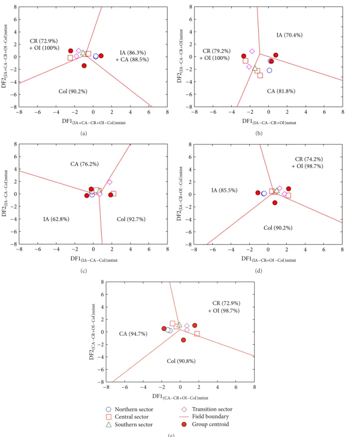
Figure 4: Discriminant-function multidimensional diagrams based on ln-transformed ratios of immobile major and trace elements for

tectonic discrimination of intermediate Sierra de las Cruces magmas.The symbols are explained as inset in (a); more details are inFigure3.

8

6

4

2

0

−2

−4

−6

−8

8

6 4 2 0 −2 −4 −6 −8

DF

2(IA

+

CA

−

CR

+

OI

−

Co

l

)

tin

t

DF1(IA+CA−CR+OI−Col)tint

CR (74.3%) +OI (100%) Col (81.0%)

IA (91.4%) +CA (90.4%)

(a)

8

6

4

2

0

−2

−4

−6

−8

8

6 4 2 0 −2 −4 −6 −8

DF

2(IA

+

CA

−

CR

+

OI

)

tin

t

DF1(IA+CA−CR+OI)tint

CR (80.5%) +OI (100%)

IA (75.7%)

CA (65.8%)

(b)

8

6

4

2

0

−2

−4

−6

−8

8

6 4 2 0 −2 −4 −6 −8

DF

2(IA

−

CA

−

Co

l

)

tin

t

DF1(IA−CA−Col)tint

Col (84.0%) IA (72.7%)

CA (64.5%)

(c)

8

6

4

2

0

−2

−4

−6

−8

8

6 4 2 0 −2 −4 −6 −8

DF

2(IA

−

CR+O

I

−

Co

l

)

tin

t

DF1(IA−CR+OI−Col)tint

CR (74.7%) +OI (100%)

Col (84.7%) IA (90.3%)

(d)

8 6

4

2

0

−2

−4

−6

−8

8 6 4 2 0

−2

−4

−6

−8

CR (74.3%)

+OI (94.1%)

Col (81.0%)

CA (95.7%)

Field boundary Group centroid Northern region

Central region Southern region Transition region DF1(CA−CR+OI−Col)tint

DF

2(CA

−

CR

+

OI

−

Co

l

)

tin

t

(e)

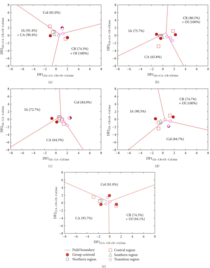
Figure 5: Discriminant-function multidimensional diagrams based on ln-transformed ratios of immobile trace elements for tectonic

discrimination of intermediate Sierra de las Cruces magmas.The symbols are explained as inset in (a); more details are inFigure3.The

8

4

0

−4

−8

8 4 0

−4

−8

CR (73.8%)

Col (75.3%)

+OI (95.4%) ₊IA (94.0%)_{CA (86.7%)}

DF

2(IA+CA

−

CR

+

OI

−

Co

l

)

macid

DF1(IA+CA−CR+OI−Col)macid

(a)

8

4

0

−4

−8

8 4

0

−4

−8

CR (83.2%)

+OI (96.9%)

IA (71.2%)

CA (79.5%)

DF

2(IA

−

CA

−

CR

+

OI

)

macid

DF1(IA−CA−CR+OI)macid

(b)

8

4

0

−4

−8

8

4 0

−4 −8

DF

2(IA

−

CA

−

Co

l

)

macid

DF1(IA−CA−Col)macid

Col (77.4%) IA (69.1%)

CA (82.3%)

(c)

8

4

0

−4

−8

8

4 0 −4 −8

CR (78.9%) +OI (96.9%)

Col (83.1%)

IA (85.5%)

DF1(IA−CR+OI−Col)macid

DF

2(IA

−

CR

+

OI

−

Co

l

)

macid

(d)

8

4

0

−4

−8

8

4 0 −4 −8

Field boundary Group centroid SC northern sector

SC central sector SC southern sector CR (73.2%)

+OI (95.4%) Col (74.1%)

CA (88.6%)

DF1(CA−CR+OI−Col)macid

DF

2(CA

−

CR

+

OI

−

Co

l

)

macid

(e)

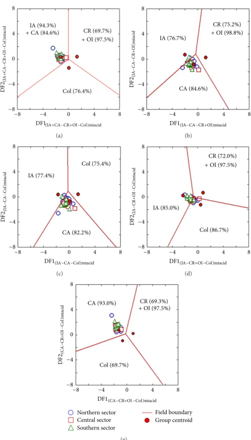
Figure 6: Discriminant-function multidimensional diagrams [22], based on ln-transformed ratios of major elements, for the tectonic

discrimination of acid Sierra de las Cruces rocks. Tectonic settings: IA: island arc, CA: continental arc, CR: continental rift, OI: ocean island,

and Col: collision.The symbols are explained as inset in (a). In (a),five groups are represented as three groups by combining IA and CA

as IA + CA and CR and OI as CR+OI.The other four diagrams ((b)–(e)) are for three groups at a time.The subscript “macid” refers to

the set of multidimensional diagrams based on ln-transformed major element (m) ratios for acid (acid) magmas. Filled circles display the

compositional centroid for each tectonic setting.The percentages in eachfield are the discrimination effectivity.The thick lines represent

equal probability discrimination boundaries in all diagrams.The coordinates of thefield boundaries and additional information are reported

IA (94.3%)

+CA (84.6%) CR (69.7%)

+OI (97.5%)

Col (76.4%) 8

4

0

−4

−8

8 4

0

−4

−8

D

F2(IA

+

CA

−

CR

+

OI

−

Co

l

)

m

tacid

DF1(IA+CA−CR+OI−Col)mtacid

(a)

8

4

0

−4

−8

8

4 0 −4 −8

DF

2(IA

−

CA

−

CR

+

OI

)

m

tacid

DF1(IA−CA−CR+OI)mtacid

IA (76.7%)

CA (84.6%)

CR (75.2%) +OI (98.8%)

(b)

8

4

0

−4

−8

8

4 0

−4 −8

DF

2(IA

−

CA

−

Co

l

)

m

tacid

DF1(IA−CA−Col)mtacid

Col (75.4%)

CA (82.2%) IA (77.4%)

(c)

8

4

0

−4

−8

8

4 0

−4 −8

DF1(IA−CR+OI−Col)mtacid

DF

2(IA

−

CR

+

OI

−

Co

l

)

m

tacid

Col (86.7%) IA (85.0%)

CR (72.0%) +OI (97.5%)

(d)

8

4

0

−4

−8

8

4 0

−4 −8

DF

2(CA

−

CR+O

I

−

Co

l

)

m

tacid

DF1(CA−CR+OI−Col)mtacid

CA (93.0%)

Col (69.7%)

CR (69.3%) +OI (97.5%)

Field boundary Group centroid Northern sector

Central sector Southern sector

(e)

Figure 7: Discriminant-function multidimensional diagrams based on ln-transformed ratios of immobile major and trace elements for

tectonic discrimination of acid Sierra de las Cruces magmas.The symbols are explained as inset in (a); more details are inFigure6.The

8

4

0

−4

−8

8 4

0

−4

−8

IA (92.6%)

+CA (60.3%)

CR (94.0%) Col (81.8%)

D

F2(IA

+

CA

−

CR

+

OI

−

Co

l

)

tacid

DF1(IA+CA−CR+OI−Col)tacid

(a)

8

4

0

−4

−8

8

4 0

−4 −8

DF

2(IA

−

CA

−

CR+O

I

)

tac

id

DF1(IA−CA−CR+OI)tacid

CA (85.5%)

IA (86.2%) CR+OI (95.7%)

(b)

8

4

0

−4

−8

8

4 0

−4 −8

DF

2(IA

−

CA

−

Co

l

)

tac

id

DF1(IA−CA−Col)tacid

CA (71.0%) Col (84.8%)

IA (83.1%)

(c)

8

4

0

−4

−8

8

4 0

−4 −8

DF

2(IA

−

CR+O

I

−

Co

l

)

tac

id

DF1(IA−CR+OI−Col)tacid

IA (91.3%)

CR+OI (97.4%)

Col (88.2%)

(d)

Field boundary Group centroid Northern sector

Central sector Southern sector

8

4

0

−4

−8

8

4 0

−4 −8

DF

2(CA

−

CR+O

I

−

Co

l

)

tac

id

DF1(CA−CR+OI−Col)tacid

Col (78.9%)

CA (74.5%)

CR+OI (93.1%)

(e)

Figure 8: Discriminant-function multidimensional diagrams based on ln-transformed ratios of immobile trace elements for tectonic

discrimination of acid Sierra de las Cruces magmas.The symbols are explained as inset in (a); more details are inFigure6.The subscript

30

25

20

15

10

5

0

Lin

ka

ge

d

ist

an

ce

SC

56

SC

55

SC

54

SC

42

SC

41

SC

45 _JQ2

SC

48

SC

51

SC

46

SC

39

SC

47

SC

40 _AJ2

SC

52 _JQ4

SC

43

CH

1

SC

49

SC

52

a

SC

49

a

SC

49

b

N1 N2

N3

(a)

16

14

12

10

8

6

4

2

0

Lin

ka

ge

d

ist

an

ce

C2 C1 C3

C4

SC

31

SC

30

SC

34

PC

2

SC

36

SC

35

SC

38

SC

35

A

SC

32 _ST1

SC

37

SC

37

A

(b) 20

15

10

5

0

Lin

ka

ge

d

ist

an

ce

ST1

ST2 ST3

SC

21

SC

28

SC

60

SC

25

SC

8

TO

1

SC

29

SC

57

SC

24

SC

10

SC

27

SC

20

SC

58

SC

59

SC

22

SC

16

SC

3

SC

53

SC

57

A

SC

24

A

TO

2

SC

26

(c)

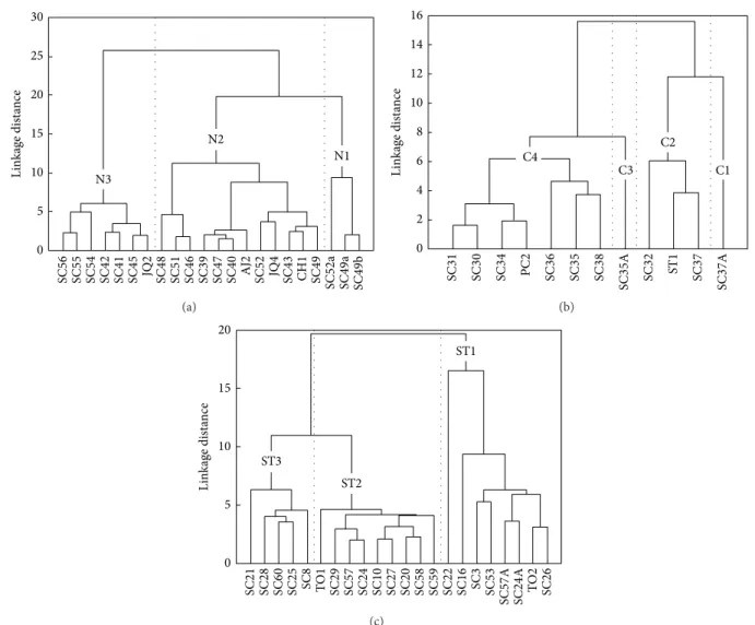
Figure 9: Dendrograms showing the results of the cluster analysis (considering Euclidean linkage distances) for the volcanic rocks from the (a) northern, (b) central, and (c) south + transition Sierra de las Cruces sectors.

as possible, whereas the differences between the clusters are as large as possible. In magma mingling scenario, this technique would be helpful for the SC sample distribution in resident, invasive, and comingled magmas.

In this work, cluster analysis was performed using the natural logarithm of major elements ([SiO2]adj–[P2O5]adj) and representative trace (transition: Co, V; rare earth: La, Eu, Yb; lithophile: Ba, Sr, U; high-field strength: Hf, Y, Zr) elements to[Al₂O₃]adjratios by using a hierarchical cluster method (HCM; [42]). Geochemical ratios were previously standardized (z-scores) by means of

𝐾𝑖𝑗=𝑋𝑖𝑗_𝑆− 𝑋

𝑖𝑐 , (1)

where𝐾𝑖𝑗is the standardized value of𝑋𝑖𝑗, the𝑖th variable for the𝑗th sample,𝑋is the mean value of the𝑖th variable, and𝑆𝑖𝑐 is its standard deviation. Additionally, the normality of each standardized variable was confirmed by the Shapiro-Wilks test. Cluster analysis applied a Ward’s linkage rule, which linked iteratively nearby points through a similarity matrix

and performed an ANOVA test to evaluate the distance between clusters [43]. The adopted procedure gives equal weight to each geochemical ratio.The measure of similarity was simply the distance as defined in Euclidean space.The distance between two samples(𝑗,𝑘)is given by

𝑑𝑗𝑘=[ 𝑁 ∑

𝑖=1(𝐾𝑖𝑗− 𝐾𝑖𝑘)

2 ]

1/2

, (2)

where𝐾𝑖𝑗denotes the𝐾th variable measured on object𝑖in sample𝑗and𝐾𝑗𝑘is the𝐾th variable measured on object𝑖in sample𝑘.The results of the cluster analysis were graphically displayed in three dendrograms with units in Euclidean values, corresponding to northern, central, and southern-transition SC sectors.

1.0

0.5

0.0

−0.5

−1.0

1.0 0.5

0.0

−0.5

−1.0

Fac

to

r

2

:

18.6

%

Factor1:57.4%

Na Si

U

K Ba

Hf Zr

La

Eu

Y

Sr Yb

P

Ti

Fe2 Fe3

V Co Mg

Mn Ca

(a)

1.0

0.5

0.0

−0.5

−1.0

1.0 0.5

0.0

−0.5

−1.0

Fac

to

r

2

:

32.0

%

Factor1:45.0%

P

Fe2

Si

Na K

Zr U Hf Ba La

Y Eu

Sr Mn

Ti_{V Ca}

CoFe3 Mg

(b)

1.0

0.5

0.0

−0.5

−1.0

1.0 0.5

0.0

−0.5

−1.0

Fac

to

r

2

:

24

.7

%

Factor1:42.8%

Fe3

Si

U K

Na

Ba Hf La

Sr Zr

Y Yb _EuP

V Ca

Ti, Fe2

Co Mn Mg

(c)

Figure 10: Projection of the variables on the factor-plane F2-F1generated by principal component analysis (PCA) for the Sierra de las Cruces sectors: (a) northern, (b) central, and (c) southern + transition.

“principal components.” Each factor will be a function of the individual contributions of the original variables [44]. The greatest variance for the transformed data was linked to thefirst principal component, whereas the second variance magnitude was related to the second principal component, and so on.The PCA considers a data matrix,X(𝑛rows×𝑝 columns; rows represent different samples, and columns give a particular chemical component; each component which has been standardized yielded a zero empirical mean).The transformation is stated by a set of 𝑝-dimensional vectors w_(𝑘)= (𝑤₁, . . . ,𝑤_𝑝)_(𝑘)that map each row vectorx_(𝑖)ofXto a

new vector of principal component factorst_(𝑖)= (𝑡₁, . . . ,𝑡_𝑝)_(𝑖) given by

t_𝑘(𝑖)=x_(𝑖)⋅w_(𝑘). (3) Individual variables of t considered over the data set successively inherit the maximum possible variance fromx, with each loadingwconstrained to be a unit vector.Thefirst principal componentw₍₁₎satisfied

w₍₁₎=arg max{∑

𝑖 (𝑡1)

2

(𝑖)}=arg max∑

𝑖 (

2.4

2.1

1.8

1.5

1.2

0.9

0.6

48 52 56 60 64 68 72

[

Fe2 O3

]adj

(%wt)

[SiO2]adj(%wt)

N = 22; R2_{= 0.97}

MIZ MPO _ISC

F_IZ FPO

FSC

[Fe2O3]adj=−0.073∗[SiO2]adj+ 5.98

(a)

48 52 56 60 64 68 72

8

6

4

2

0

[

FeO

]adj

(%wt)

[SiO2]adj(%wt)

N = 22; R2_{= 0.97}

MIZ

MPO

FPO

I_SC

F_SC FIZ

[FeO]adj=−0.267∗[SiO2]adj+ 20.54

(b)

48 52 56 60 64 68 72

12

10

8

6

4

2

0

[

MgO

]adj

(%wt)

[SiO2]adj(%wt)

N = 22; R2= 0.93 MIZ

M_PO

ISC

FPO

F_SC FIZ

[MgO]_adj=−0.437∗[SiO2]adj+ 31.2

(c)

48 52 56 60 64 68 72

0.14

0.12

0.10

0.08

0.06

0.04

[

Mn

O

]adj

(%wt)

[SiO2]adj(%wt)

N = 22; R2= 0.96

MIZ

MPO

I_SC

FIZ

FPO

F_SC M_{IZ [MnO]}

adj=−0.0038∗[SiO2]adj+ 0.318

(d)

48 52 56 60 64 68 72

9

8

7

6

5

4

3

2

[

CaO

]adj

(%wt)

[SiO2]adj(%wt)

N = 22; R2_{= 0.90} MIZ

MPO

ISC

F_IZ FPO

F_SC

N1 N2 N3

[CaO]adj=−0.238∗[SiO2]adj+ 19.9

(e)

48 52 56 60 64 68 72

2.8

2.4

2.0

1.6

1.2

0.8

[

K2

O

]adj

(%wt)

[SiO2]adj(%wt)

N = 22; R2_{= 0.89}

MIZ

MPO

I_SC

FIZ

F_PO

F_SC

N1 N2 N3

[K2O]adj= 0.093∗[SiO2]adj−3.84

(f)

Figure 11: Major element Harker-type diagrams for volcanic rocks from the Sierra de las Cruces northern sector. An ordinary least-squares

(OLS) regression model is included in each diagram (OLS equation;𝑁is number of samples;𝑅2_{is Pearson regression coefficient; solid line}

is OLS model; discontinuous lines are95% confidence regression bands). Abbreviations for end-members in mixing/mingling models: (a)

Sierra de las Cruces:𝐼SC: intermediate and𝐹SC: felsic; (b)Iztacc´ıhuatl volcano[31]:𝑀IZ: mafic and𝐹IZ: felsic; (c)Popocat´epetl volcano[32]:

N = 22; R2_{= 0.87} I_SC

FSC

[SiO2]adj(%wt)

400

300

200

100

0

52 56 60 64 68 72

Cr (p

pm)

Cr=−20.87∗[SiO2]adj+ 1461

N1 N2 N3

(a)

N = 22; R2_{= 0.97}

MSC

F_SC

[SiO2]adj(%wt)

52 56 60 64 68 72

50

40

30

20

10

0

C

o (

pp

m)

N1 N2 N3

Co=−1.89∗[SiO2]adj+ 136

(b)

N = 22; R2_{= 0.83}

ISC

FSC

[SiO2]adj(%wt)

52 56 60 64 68 72

120

80

40

0

N

i (p

pm)

N1 N2 N3

Ni=−5.82∗[SiO2]adj+ 422

(c)

N = 22; R2= 0.95

[SiO2]adj(%wt)

52 56 60 64 68 72

240

200

120 160

80

40

V

(p

pm)

N1 N2 N3

V=−8.52∗[SiO2]adj−647

(d)

Figure 12: Trace element Harker-type diagrams for volcanic rocks from the Sierra de las Cruces northern sector. OLS regression models as

those presented inFigure11.

where the quantity to be maximized is known as Rayleigh quotient.The𝑘th component was determined by subtracting the𝑘–1principal components fromX:

̂

X_𝑘−1=X−

𝑘−1

∑

𝑠=1

Xw_(𝑠)w₍T_𝑠). (5)

The vector associated with this component and showing the maximum variance from this new matrix would be defined as

w_(𝑘)=arg max {󵄩󵄩󵄩󵄩󵄩̂X_𝑘−1w󵄩󵄩󵄩󵄩_󵄩2}. (6) All calculations related to cluster analysis were carried out using the STATISTICA for Windows software.

4.5. Mass-Balance Evaluations. Nixon [31] applied a simple mass-balance scheme for the quantitative characterization of binary mixtures and end-member compositions in the Iztacc´ıhuatl volcano (central MVB). The author suggested that, despite the compositional heterogeneity, if a chemical component can be found whose concentration is invariant in time and known in the mix and in each of the end-members, it is possible to treat quantitatively the magma mixing process.

1.0

0.8

0.6

0.4

0.2

0.0

1.0 0.8

0.6 0.4

0.2 0.0

Intermediate end-member proportion

In

ter

m

ed

ia

te e

nd

-m

em

be

r p

ro

po

rt

io

n

QFe2

QSi

(a)

1.0

0.8

0.6

0.4

0.2

0.0

1.0 0.8

0.6 0.4

0.2 0.0

Intermediate end-member proportion

In

ter

m

ed

ia

te e

nd

-m

em

be

r p

ro

po

rt

io

n

Q_Si QMg

(b)

1.0

0.8

0.6

0.4

0.2

0.0

1.0 0.8

0.6 0.4

0.2 0.0

Intermediate end-member proportion

In

ter

m

ed

ia

te e

nd

-m

em

be

r p

ro

po

rt

io

n

Q_Si QCo

(c)

1.0

0.8

0.6

0.4

0.2

0.0

1.0 0.8

0.6 0.4

0.2 0.0

Intermediate end-member proportion

In

ter

m

ed

ia

te e

nd

-m

em

be

r p

ro

po

rt

io

n

QSi

Q_V

(d)

Figure 13: Mean proportions of mafic end-members in the comingled lavas from the Sierra de las Cruces, calculated using the mass-balance

equation𝑄𝑖

𝐴 = |𝐶𝑖𝑀− 𝐶𝑖𝐵|/|𝐶𝑖𝐴− 𝐶𝑖𝐵|[31] for[SiO2]adj,[FeO]adj,[MgO]adj, Co, and V. Proportions determined using[SiO2]adjare plotted

against those obtained using the other constituents.The diagonal line indicates perfect agreement between results.

amount of a component in the mixed lava could be repre-sented by

𝑄𝑖_𝐴= 󵄨󵄨󵄨󵄨󵄨𝐶 𝑖

𝑀− 𝐶𝑖𝐵󵄨󵄨󵄨󵄨_󵄨

󵄨󵄨󵄨󵄨𝐶𝑖

𝐴− 𝐶𝑖𝐵󵄨󵄨󵄨󵄨,

(7)

where 𝑄𝑖

𝐴 +𝑄𝑖𝐵 = 1, and𝑄𝑖 and 𝐶𝑖 represent the weight fraction and concentration, respectively, of element 𝑖 in subscripted end-members 𝐴 and 𝐵 and mixture 𝑀. The composition of an end-member could be estimated by

𝐶𝑗_𝐴=󵄨󵄨󵄨󵄨󵄨𝐶 𝑗

𝑀− 𝑄𝑖𝐵𝐶𝑗𝐵󵄨󵄨󵄨󵄨_󵄨

𝑄𝑖

𝐴 ,

(8)

where constituent 𝑖 ̸=𝑗. In this work, this mass-balance approach (model A) was applied to SC lavas, being restricted to those sectors where the end-member compositions were available and to those components that exhibit a statistically significant linear coherence in [SiO2]adj-Harker diagrams. This test involved the evaluation, at99% confidence level, of

Pearson product-moment correlation coefficient(𝑟)and the sample size (𝑛). Details and required caution in the use of𝑟

have been reported in Bevington and Robinson [45]. On the other hand, Zou [33] reported a mass-balance approach to explain the 𝑦𝑚 = (𝑢/𝑎)𝑚 and 𝑥𝑚 = (V/𝑏)𝑚 geochemical ratios (where 𝑎, 𝑏, 𝑢, and V represent major or trace elements) in SC comingled lavas as a product of a mixture of two components 1 and 2. The variation in the

𝑦𝑚 and 𝑥𝑚 geochemical ratios could be modeled by the hyperbolic equation (condition𝑎1/𝑎2≠𝑏1/𝑏2):

Table 2: Major element composition (% m/m) and CIPW norm for the volcanic rocks from the Sierra de las Cruces rangea_.

Sample SC03 SC16 SC22 SC46 SC51 SC52 SC52a SC53 SC58 SC60

Sector SCT SCT SCT SCN SCN SCN SCN SCS SCS SCS

TAS D A BTA D D D BA A D D

Major-element measured composition (% m/m)

SiO2 60.88 54.64 53.44 64.29 65.91 60.73 48.34 54.81 63.21 66.71

TiO2 0.981 0.912 1.542 0.661 0.583 0.785 1.636 1.128 0.695 0.582

Al2O3 16.72 19.80 15.51 15.98 15.24 16.10 16.91 18.99 16.89 15.85

Fe2O3t 4.57 5.43 8.66 4.28 4.00 5.43 9.35 6.67 5.00 3.90

MnO 0.099 0.092 0.136 0.065 0.061 0.062 0.105 0.103 0.073 0.062

MgO 6.12 2.23 6.71 1.52 2.02 2.43 6.59 2.34 1.37 1.68

CaO 5.57 2.66 7.43 3.69 3.87 4.44 5.56 4.59 4.30 3.90

Na2O 2.97 3.47 3.98 4.07 4.01 4.01 2.36 3.68 4.40 4.56

K2O 0.80 0.80 1.53 2.50 2.52 1.89 1.30 0.84 1.68 2.23

P2O5 0.14 0.22 0.63 0.18 0.18 0.21 0.19 0.26 0.13 0.17

LOI 0.60 8.95 0.11 2.70 2.30 3.01 7.59 7.01 3.06 0.24

Total 99.430 99.204 99.678 99.906 100.704 99.097 99.931 100.421 100.808 99.884

CIPW norm

Q 18.730 23.358 — 20.600 21.530 16.476 5.223 16.302 18.988 20.458

Or 4.621 5.260 9.142 15.123 15.182 11.672 8.386 5.342 10.194 13.261

Ab 25.520 32.678 34.050 35.539 34.591 35.463 21.797 33.517 38.230 38.839

An 27.132 13.089 20.155 17.677 16.451 21.265 28.762 22.684 21.039 16.298

C 1.230 9.925 — 0.330 — — 2.145 4.633 0.333 —

Di — — 10.431 — 1.568 0.264 — — — 1.685

Hy 18.933 11.093 18.543 7.305 7.560 10.617 26.668 12.075 7.579 6.444

Ol — — 0.202 — — — — — — —

Mt 1.612 2.099 3.040 1.695 1.564 2.178 3.146 2.494 1.970 1.506

Il 1.892 1.928 2.961 1.295 1.128 1.557 3.392 2.306 1.356 1.113

Ap 0.329 0.568 1.476 0.431 0.424 0.507 0.480 0.649 0.308 0.396

Mg-v 77.719 51.684 66.871 48.905 57.634 54.66 63.940 47.752 42.473 53.718

FeOt_{/MgO 0.672 2.191 1.161 2.533 1.782 2.01 1.277 2.565 3.283 2.089}

a_{TAS: rock classification following the Le Bas et al [36] scheme. A: andesite, BA: basaltic andesite, BTA: basaltic trachyandesite, and D: dacite.}

Adjusted composition (% m/m) and CIPW norm calculated applying SINCLAS program [14,15]. Mg-v =100∗Mg+2_/(Mg+2_{+ 0.9∗[Fe}+2_+Fe+3_{]), atomic;}

Fe+2_{and Fe}+3_{calculated from adjusted FeO and Fe}

2O3following Middlemost [34]. In this model, the𝐴to𝐷coefficients have been defined as

𝐴= 𝑎2𝑏1𝑦2− 𝑎1𝑏2𝑦1, (10a) 𝐵= 𝑎1𝑏2− 𝑎2𝑏1, (10b) 𝐶= 𝑎2𝑏1𝑥1− 𝑎1𝑏2𝑥2, (10c) 𝐷= 𝑎1𝑏2𝑥2𝑦1− 𝑎2𝑏1𝑥1𝑦2, (10d)

where the geochemical ratios in the components1and2are

𝑥1= V_𝑏1

1, (11a)

𝑥2= V_𝑏2

2, (11b)

𝑦1= 𝑢_𝑎1

1, (11c)

𝑦2= 𝑢_𝑎2

2. (11d)

The proportion of thefirst component could be estimated by

𝑓1= _(𝑎 −𝑎2𝑦𝑚+𝑎2𝑦2

1− 𝑎2) 𝑦𝑚− 𝑎1𝑦1+𝑎2𝑦2. (12)

In this work, the scheme described by Zou ([33], model B) was applied to evaluate the mixing/mingling process in the SC northern sector. All calculations of mixing models were carried out using the STATISTICA for Windows software.

5. Results

Table 3: Trace element composition (ppm) for the volcanic rocks from the Sierra de las Cruces range.

Sample SC03 SC16 SC22 SC46 SC51 SC52 SC52a SC53 SC58 SC60

Sector SCT SCT SCT SCN SCN SCN SCN SCS SCS SCS

TAS D A BTA D D D BA A D D

La 14.1 20.0 34.8 23.4 25.2 24.1 16.2 18.8 11.1 17.1

Ce 31.2 47.9 77.8 41.2 40.6 38.2 40.9 41.2 21.8 34.1

Pr 4.03 7.28 10.10 6.54 6.12 6.71 5.19 5.14 2.99 4.35

Nd 17.1 29.7 42.9 26.5 24.7 28.4 24.3 21.6 12.6 17.4

Sm 3.9 6.1 9.0 5.4 4.8 5.6 5.5 4.6 2.9 3.6

Eu 1.24 1.77 2.67 1.52 1.37 1.66 1.65 1.57 1.08 1.10

Gd 3.9 6.2 8.0 4.4 4.3 5.0 5.3 4.6 2.9 3.3

Tb 0.6 0.9 1.1 0.7 0.7 0.7 0.8 0.7 0.5 0.5

Dy 3.3 5.2 5.7 3.8 3.7 4.0 4.6 3.9 2.6 2.7

Ho 0.7 1.0 1.0 0.7 0.7 0.8 0.9 0.8 0.5 0.5

Er 1.9 2.7 2.9 2.0 2.1 2.2 2.5 2.2 1.5 1.6

Tm 0.28 0.37 0.42 0.30 0.30 0.30 0.36 0.32 0.22 0.22

Yb 1.7 1.8 2.5 2.0 1.9 1.9 2.2 1.9 1.4 1.4

Lu 0.24 0.32 0.40 0.30 0.30 0.29 0.33 0.29 0.23 0.21

Sc 15 19 11 9 15 37 18 13 8

V 102 39 150 88 75 109 216 119 59 51

Cr 246 28 260 60 60 150 360 150 170 40

Co 18 10 29 10 9 15 40 21 15 9

Ni 88 110 30 30 50 110 80 50 20

Cu 21 94 30 10 20 20 60 20 20

Ga 13 22 20 18 20 21 22 24 21 21

Rb 13 3 28 59 61 40 22 6 38 58

Sr 380 303 763 521 502 582 445 569 454 368

Y 20 32 28 20 21 19 22 21 15 18

Zr 136 156 237 156 160 158 162 194 143 149

Nb 6.0 5.4 17.0 4.0 4.0 3.0 3.0 8.0 13.0 4.0

Cs 2.1 2.8 2.7 1.1 1.2 2.1

Ba 276 412 648 542 571 481 344 660 388 481

Hf 3.4 4.4 5.4 4.2 4.2 4.4 4.7 4.8 3.8 4.2

Ta 0.40 0.33 1.10 0.5 0.5 0.30 0.20 0.7 0.3 0.6

Pb 72 11 11 14 11 23 10 9 11

Th 1.8 3.0 4.1 6.7 6.7 4.0 3.0 5.0 3.4 8.2

U 0.6 1.3 1.2 2.6 2.5 1.6 1.1 1.1 1.4 3.1

10; Table4 and Figure3) showed a collisional setting with total percent probability value (% prob) of about 45.8%. However, immobile major and trace element based diagrams (𝑛= 9;Table4andFigure4) indicated a within-plate regime, although with a relatively low % prob of only about 38.1. Unlike other sets of diagrams, a continental arc setting can be inferred from those based on immobile trace elements (𝑛= 10; % prob =39.7;Table4 andFigure5). It is important to note that intermediate samples from southern and transition sectors (1.9to0.5Ma) represent the main contribution to the collisional and within-plate settings.

A relatively large number of samples (𝑛 = 46) from SC database proved to be of acid magma. In contrast to intermediate magmas, all diagrams indicated a subduction-related setting for the SC acid magmas, with total percent

probability values for this tectonic regime of about74.1%, 63.0%, and68.7%, respectively, for the major, major and trace, and trace element based diagrams (Table5and Figures6,7, and8).The results of the tectonic setting are further evaluated from discordancy and significance tests in the Discussion section below.

T ab le 5 :T ec to ni cd isc rim in at io n an al ys is of fe lsi cm ag m as fro m th eS ie rr ad el as Cr uc es us in g m ul tid im en sio na ld ia gr am s[ 22 ] a . Fi gu re na m e Fi gu re ty pe To ta ln um be ro fs am pl es N um be ro fd isc rim in at ed sa m pl es Ar c Wi th in -p la te C ol lis io n IA + CA [ 𝑥 ± 𝑠 ] (

𝑝IA+C

Table 6: Statistical parameters of major (%wt) and trace (ppm) element composition for the Sierra de las Cruces magmatic clusters. (a)

Element N1(𝑛= 3) Northern SC sector (N2(𝑛= 12) 𝑛= 22) N3(𝑛= 7)

𝑥 Min. Max. s 𝑥 Min. Max. s 𝑥 Min. Max. s

[SiO2]adj 57.6 52.77 60.38 4.2 65.1 63.25 67.19 1.5 69.0 67.94 69.98 0.8

[TiO2]adj 1.1 0.71 1.79 0.6 0.69 0.59 0.82 0.07 0.522 0.486 0.552 0.031

[Al2O3]adj 16.5 15.38 18.46 1.7 16.2 15.54 16.83 0.5 15.9 15.11 16.49 0.5

[Fe2O3]adj 1.68 1.42 2.17 0.42 1.23 1.08 1.50 0.13 0.89 0.83 0.96 0.05

[FeO]adj 5.1 4.05 7.23 1.8 3.08 2.70 3.76 0.33 2.22 2.08 2.39 0.11

[MnO]adj 0.103 0.095 0.115 0.011 0.070 0.059 0.082 0.008 0.0574 0.053 0.060 0.0026

[MgO]adj 6.7 6.23 7.19 0.5 2.5 1.15 4.17 0.8 1.11 0.698 1.577 0.30

[CaO]adj 6.34 6.07 6.59 0.26 4.4 3.41 5.18 0.5 3.31 3.08 3.79 0.30

[Na2O]adj 3.3 2.58 3.66 0.6 4.28 4.09 4.53 0.13 4.37 4.20 4.48 0.11

[K2O]adj 1.442 1.419 1.462 0.022 2.23 1.84 2.61 0.30 2.51 2.29 2.80 0.19

[P2O5]adj 0.164 0.143 0.207 0.037 0.193 0.151 0.292 0.036 0.1344 0.130 0.141 0.0043

La 14.0 12.3 16.2 2.0 20 13.6 34.8 6 19.8 15.1 23.6 3.2

Eu 1.26 1.03 1.65 0.34 1.32 1.04 2.15 0.32 1.07 0.91 1.25 0.12

Yb 1.90 1.60 2.20 0.30 1.76 1.26 2.70 0.40 1.52 1.16 1.70 0.22

Ba 344 329 358 15 500 414 571 60 530 472 578 50

Co 28 22 40 10 12.3 9.0 16.0 2.2 6.4 6.0 7.0 0.5

Cr 290 230 360 70 90 60 160 34 32 20 40 7

Hf 3.5 2.9 4.7 1.0 3.96 3.20 4.60 0.40 4.13 3.8 4.7 0.39

Sr 459 445 474 15 520 431 601 60 410 351 566 70

Th 2.87 2.80 3.00 0.12 5.3 3.6 6.7 1.2 6.0 3.4 8.2 1.4

U 1.03 0.90 1.10 0.12 2.10 1.40 2.60 0.44 2.4 1.10 3.00 0.6

V 160 123 216 50 92 75 109 10 60 52 73 7

Y 20.7 18 22 2.3 19 12 34 6 16.1 12.0 22.0 3.2

Zr 122 100 162 35 146 109 162 15 151 133 184 18

(b)

Element _C1( Central SC sector (𝑛= 12)

𝑛= 1) C2(𝑛= 3) C3(𝑛= 1) C4(𝑛= 7)

𝑥 Min. Max. s 𝑥 Min. Max. s

[SiO2]adj 58.329 65.1 63.76 67.30 1.9 61.338 64.2 63.61 65.16 0.5

[TiO2]adj 1.109 0.71 0.63 0.77 0.08 0.791 0.69 0.65 0.78 0.05

[Al2O3]adj 17.043 16.3 15.89 16.84 0.5 17.400 16.46 15.99 17.10 0.40

[Fe2O3]adj 1.778 1.24 1.08 1.35 0.15 1.424 1.29 1.16 1.57 0.13

[FeO]adj 5.079 3.11 2.70 3.36 0.36 4.068 3.23 2.90 3.91 0.33

[MnO]adj 0.118 0.0783 0.0760 0.0810 0.0025 0.071 0.078 0.070 0.088 0.007

[MgO]adj 3.663 2.2 1.51 3.06 0.8 3.918 3.0 2.31 3.61 0.5

[CaO]adj 6.764 4.5 3.79 5.23 0.7 4.962 4.78 3.97 5.37 0.42

[Na2O]adj 4.290 4.35 4.27 4.49 0.12 4.270 4.36 4.16 4.62 0.17

[K2O]adj 1.497 2.163 2.136 2.180 0.023 1.592 1.77 1.66 1.95 0.11

[P2O5]adj 0.329 0.21 0.16 0.24 0.05 0.165 0.157 0.141 0.165 0.009

La 26.8 26.0 23.6 27.7 2.2 11.1 14.3 12.1 19.1 2.3

Eu 2.09 1.68 1.45 2.12 0.38 1.10 1.07 0.99 1.34 0.12

(b) Continued.

Element Central SC sector (𝑛= 12)

C1(𝑛= 1) C2(𝑛= 3) C3(𝑛= 1) C4(𝑛= 7)

𝑥 Min. Max. s 𝑥 Min. Max. s

Ba 507 550 485 602 60 309 400 364 447 29

Co 26 13.0 10.0 15.0 2.6 17 13.9 12.0 17.0 2.0

Hf 3.90 3.73 3.60 3.90 0.15 3.20 3.59 3.40 3.70 0.11

Sr 813 600 434 683 140 453 469 451 507 21

U 1.70 1.94 1.80 2.02 0.12 1.20 1.38 1.00 1.70 0.22

V 150 89 71 103 16 100 88 81 99 7

Y 24.0 19.7 17.0 21.0 2.3 14.0 15.6 13.0 20.0 2.2

Zr 138 137.7 137 139 1.2 114 131 123 138 6

(c)

Element ST1(𝑛= 8) Southern and transition SC sectors (ST2(𝑛= 9) 𝑛= 22) ST3(𝑛= 5)

𝑥 Min. Max. 𝑠 𝑥 Min. Max. 𝑠 𝑥 Min. Max. 𝑠

[SiO2]adj 59.3 54.03 61.83 2.5 64.6 63.30 65.97 0.9 67.4 64.92 69.41 1.8

[TiO2]adj 1.09 0.84 1.56 0.23 0.72 0.63 0.92 0.09 0.61 0.54 0.66 0.05

[Al2O3]adj 18.1 15.68 22.04 2.1 16.7 15.76 17.75 0.6 16.26 15.95 17.04 0.44

[Fe2O3]adj 1.59 1.11 2.10 0.28 1.28 1.11 1.44 0.12 1.03 0.86 1.17 0.13

[FeO]adj 4.5 3.18 5.99 0.8 3.21 2.78 3.61 0.30 2.58 2.14 2.92 0.33

[MnO]adj 0.105 0.079 0.138 0.018 0.071 0.052 0.088 0.014 0.054 0.022 0.079 0.021

[MgO]adj 4.0 2.48 6.78 1.7 2.3 1.41 3.51 0.7 1.6 0.49 2.81 1.0

[CaO]adj 5.6 2.96 7.51 1.4 4.53 4.04 5.11 0.39 3.9 3.23 4.87 0.7

[Na2O]adj 4.00 3.02 4.39 0.44 4.51 4.28 4.77 0.14 4.34 4.05 4.59 0.26

[K2O]adj 1.33 0.78 2.01 0.43 1.84 1.63 2.09 0.15 2.19 1.94 2.35 0.15

[P2O5]adj 0.27 0.14 0.64 0.16 0.17 0.11 0.25 0.05 0.155 0.135 0.177 0.018

La 18 11.5 34.8 7 14.5 11.1 18.2 2.2 19.0 16.9 25.2 3.5

Eu 1.6 1.13 2.67 0.5 1.13 1.04 1.34 0.09 1.24 1.10 1.49 0.16

Yb 2.0 1.3 2.7 0.5 1.52 1.01 2.30 0.34 1.74 1.40 2.10 0.30

Ba 420 276 660 150 416 369 471 37 469 434 499 25

Co 19 10 29 5 12.9 10.0 20.0 3.3 8.8 5.0 12.0 2.9

Hf 4.2 3.4 5.4 0.7 3.68 3.30 4.10 0.24 3.90 3.60 4.20 0.28

Sr 500 303 763 130 474 416 533 40 410 364 495 50

U 1.04 0.60 1.32 0.28 1.50 0.80 2.00 0.34 2.0 1.5 3.1 0.6

V 110 39 150 33 83 59 96 12 69 51 84 12

Y 23 13.0 32.2 6 14.9 11.0 17.0 1.8 22 16 36 8

Zr 162 129 237 38 136 125 149 8 148 126 164 14

The studied rocks from northern SC sector (Table6; Figure9(a)) were distributed in three general clusters (N1 [13.6%], N2[54.5%], and N3[31.9%]).The PCA calculation indicated that the ∼94.2% of geochemical variability of samples from northern SC sector could be explained by three factors.The factor F1contributed with57.4%, being associated with major (excepting Na and P) and transition elements; rare earth elements and yttrium ruled a contribution of 18.6% by means of the factor F2(Figure10(a)).The principal component F3(a function of Na, P, and Sr) explained the8.2% of the chemical variability.

The samples from central SC conformed four groups (C1 [8.3%], C2[25.0%], C3[8.3%], and C4[58.3%];Table6and Figure9(b)). A ∼94.1% of the chemical variability can be

explained by means of five factors. The factor F1 (45.0%) is controlled by Si and alkali composition. A 32.0% of the compositional heterogeneity has been associated with the incompatible elements using the principal component F2 (Figure10(b)).The factor F3(ruled by Mg, Ca, and HFSE) contributed with a10.6%.

Table 7:𝐴–𝐷coefficients of hyperbolic Equations (10a)–(10d) for magma mixing between N1and N3end-members (northern Sierra de las

Cruces sector), generated applying the mass-balance model by Zou [33].

Ratio-ratio system 𝑦-axis 𝑥-axis Hyperbolic mixing equation coefficients

𝐴 𝐵 𝐶 𝐷

1 [Fe2O3]adj/[K2O]adj [SiO2]adj/[FeO]adj 0.81 −9.60 45.1 64.7

2 [Fe2O3]adj/[Al2O3]adj [SiO2]adj/[FeO]adj 0.81 −44.5 −223 64.7

3 V/Ba [SiO2]adj/[FeO]adj −49.2 −1939 6792 7584

4 V/U [SiO2]adj/[FeO]adj −49.2 −9.95 67.2 7584

5 Cr/Th [SiO2]adj/[FeO]adj −481 −24.2 148 18168

6 Cr/Yb [SiO2]adj/[FeO]adj −481 −3.53 −43.5 18167

7 [MgO]adj/Eu [SiO2]adj/V −224 −96 −25.3 398

8 [MgO]adj/Hf [SiO2]adj/V −225 −451 −3.61 398

9 [CaO]adj/Ta [SiO2]adj/V 149 −66 12.7 247

10 [CaO]adj/Zr [SiO2]adj/V 149 −16840 280 247

11 Ga/Ni [SiO2]adj/V 2038 2600 −5518 167

12 Ga/Rb [SiO2]adj/V 2037 −8280 1685 167

1.0

0.8

0.6

0.4

0.2

0.0

63 64 65 66 67

M

a

fi

c e

nd

-m

em

be

r p

ro

po

rt

io

n

SC

49

SC

52

SC

43

JQ

4 CH

1

SC

47

SC

40

AJ

2

SC

39

SC

46

SC

48

SC

51

[SiO2]_adj(%wt)

Model A (Nixon,1988[31])

Model B (Zou,2007[33])

Figure 14: Mean±one standard deviation of intermediate

end-member proportions (N1) in the comingled lavas (N2) from the

Sierra de las Cruces northern sector versus[SiO₂]adj, produced by

the incomplete mixing of N1and N3end-members: (a) redfilled

circle and line calculated (𝑛= 11) from the mass-balance approach

proposed by Nixon [31] and (b) bluefilled square and line calculated

(𝑛= 12) from the mass-balance approach proposed by Zou [33].

(Figure10(c)). An 11.9% of the chemical heterogeneity is explained by the factor F3, a variable ruled by Na, K, and V composition.

The mass-balance approach for magma mixing (model A) used by Nixon [31] was applied to the geochemical data from SC northern sector (i.e., intermediate N1cluster interacting with felsic N3 group resulting in N2 comingled lavas). The mixing analysis was essentially limited to [SiO2]adj, [Fe2O3]adj,[FeO]adj,[MnO]adj,[MgO]adj,[CaO]adj,[K2O]adj, Co, Cr, Ni, and V, since all these constituents exhibit a statistically significant linear coherence in Harker diagrams

(𝑟 = 0.89–0.98; 𝑛 = 22; statistically significant at 99%

confidence level; Figures11and12) and have relatively small concentration ranges in felsic N3end-member (Table6).

The proportion of the intermediate N1 end-member in each N2 mixed lava was calculated using (7) and the average composition of the intermediate (𝐼SC) and felsic (𝐹SC) end-members. Calculated proportions exhibit inter-nal consistency for majority of the chemical components (Figure13). For each sample, the estimated proportions display a Gaussian distribution (their normality behavior was proved by a Schapiro-Wilks test), covering between∼15and 47% in average proportion of the andesitic N1end-member (Figure14).

On the other hand, the mixing model B [33] was applied to lavas of the northern SC sector.The coefficients

𝐴 to 𝐷 ((10a)–(10d)) of the hyperbolic mixing equation (9) were established for twelve geochemical ratio-ratio

𝑢/𝑎–V/𝑏 systems (Table7): (1)𝑢/𝑎: [Fe₂O₃]adj/[K2O]adj, [Fe₂O₃]adj/[Al2O3]adj, V/Ba, V/U, Cr/Th, and Cr/Yb –V/𝑏: [SiO₂]adj/[FeO]adj; (2)𝑢/𝑎 : [MgO]adj/Eu, [MgO]adj/Hf, [CaO]adj/Ta, [CaO]adj/Zr, Ga/Ni, and Ga/Rb –V/𝑏: [SiO2]adj/V). Figures 15 and 16 show some examples of the ratio-ratio diagrams for the SCN lavas, including the average composition of the intermediate (𝐼SC) and felsic (𝐹SC) end-members (blackfilled square and circle) and their hyperbolic mixing models (black solid line).The application of model B revealed that the percentages (100∗𝑓1) of the

component N1 in each of the comingled lavas N2 range from11to58% (Figure14). Each mean and its uncertainty were estimated from a statistic sample of twelve ratio-ratio systems displaying a Gaussian behavior (normality proved by a Schapiro-Wilks test).

6. Discussion

1.6

1.2

0.8

0.4

0.0

10 20 30

[SiO2]_adj/[FeO]adj

[

Fe2 O3 ]adj

/[

K2

O

]adj N1

N3

(a)

0.6

0.4

0.2

0.0

10 20 30

[SiO2]_adj/[FeO]adj

V

/

Ba

N1

N3

(b)

120

80

40

0

10 20 30

[SiO2]_adj/[FeO]_adj

Cr

/

Th N1

N3

(c)

2

1

0

0.0 0.5 1.0 1.5

[

MgO

]adj

/

Hf

[SiO2]adj/V

N1

N3

(d) 0.08

0.06

0.04

0.02

0.00

0.0 0.5 1.0 1.5

N1

N1

N2 N3

N3

[

CaO

]adj

/

Zr

[SiO2]adj/V

(e)

1.2

0.9

0.6

0.3

0.0 0.5 1.0 1.5

N1 N1

N2 N3

N3

Ga

/

Rb

[SiO2]adj/V

(f)

Figure 15: Geochemical ratio-ratio diagrams of the Sierra de las Cruces northern sector that include hyperbolic mixing models (black

solid line) between average intermediate N1 lavas (black filled circle, 𝐼SC) and average felsic N3 lavas (black filled square, 𝐹SC): (a)

[Fe2O3]adj/[K2O]adj–[SiO2]adj/[FeO]adj; (b) V/Ba –[SiO2]adj/[FeO]adj; (c) Cr/Th–[SiO2]adj/[FeO]adj; (d)[MgO]adj/Hf –[SiO2]adj/V; (e)

[CaO]adj/Zr –[SiO2]adj/V; (f) Ga/Rb –[SiO2]adj/V. Hyperbolic mixing equations, generated following the mass-balance approach by Zou

N1

N3

[SiO2]adj/[FeO]adj

[

Fe2 O3 ]adj

/[

Al2 O3 ]adj

0.12

0.10

0.08

0.06

0.04

10 20 30

(a)

N1

N3

[SiO2]adj/[FeO]adj

V

/

U

10 20 30

200

150

100

50

0

(b)

N1

N3

[SiO2]_adj/[FeO]adj

Cr

/

Yb

10 20 30

200

150

100

50

0

(c)

N1

N3

[

MgO

]adj

/

Eu

[SiO2]adj/V

0.0 0.5 1.0 1.5

8

6

4

2

0

(d)

N1

N3

[

CaO

]adj

/

Ta

[SiO2]adj/V

0.0 0.5 1.0 1.5

40

30

20

10

0

N1 N2 N3

(e)

N1

N3

Ga

/

Ni

[SiO2]adj/V

N1 N2 N3 1.2

0.9

0.6

0.3

0.0

0.0 0.5 1.0 1.5

(f)

Figure 16: Geochemical ratio-ratio diagrams of the Sierra de las Cruces northern sector that include hyperbolic mixing models (black

solid line) between average intermediate N1 lavas (black filled circle, 𝐼SC) and average felsic N3 lavas (black filled square, 𝐹SC): (a)

[Fe2O3]adj/[Al2O3]adj –[SiO2]adj/[FeO]adj; (b) V/U –[SiO2]adj/[FeO]adj; (c) Cr/Yb –[SiO2]adj/[FeO]adj; (d)[MgO]adj/Eu –[SiO2]adj/V; (e)

[CaO]adj/Ta –[SiO2]adj/V; (f) Ga/Ni –[SiO2]adj/V. Hyperbolic mixing equations, generated following the mass-balance approach by Zou [33],

Table 8: Results of the application of significance tests of Fisher𝐹and Student𝑡to the acid rock data from the Sierra de las Cruces at the

strict99% confidence level (CL) prepared from Excel output of UDASYS [37].

Element Group A Group B 𝑛A 𝑛B Df Sign 𝑡calc

𝑡criteria

One-sided

H0

One-sided

CL𝑡

One-sided

𝑡criteria

Two-sided

H0

Two-sided

CL𝑡

Two-sided (a) Major

elements

[SiO2]adj Gr2 Gr1 32 11 41.0 − 0.471 2.421 True <50 2.701 True <50

[TiO2]adj Gr2 Gr1 32 11 41.0 − 0.509 2.421 True <50 2.701 True <50

[Al2O3]adj Gr2 Gr1 32 11 41.0 − 0.687 2.421 True 72.5 2.701 True 44.9

[Fe2O3]adj Gr2 Gr1 32 11 41.0 + 0.571 2.421 True <50 2.701 True <50

[FeO]adj Gr2 Gr1 32 11 41.0 + 0.575 2.421 True <50 2.701 True <50

[MnO]adj Gr2 Gr1 32 11 12.0 + 1.599 2.680 True 93.2 3.053 True 86.4

[MgO]adj Gr2 Gr1 32 11 41.0 + 0.612 2.421 True <50 2.701 True <50

[CaO]adj Gr2 Gr1 32 11 41.0 + 0.602 2.421 True <50 2.701 True <50

[Na2O]adj Gr2 Gr1 32 11 41.0 − 1.877 2.421 True 96.6 2.701 True 93.2

[K2O]adj Gr2 Gr1 32 11 41.0 + 0.917 2.421 True 81.7 2.701 True 63.3

[P2O5]adj Gr2 Gr1 31 11 40.0 + 0.431 2.423 True <50 2.705 True <50

(b) Trace elements

La Gr2 Gr1 32 10 39.1 + 2.661 2.425 False 99.4 2.707 True 98.9

Ce Gr2 Gr1 32 11 41.0 + 1.915 2.421 True 96.9 2.701 True 93.8

Pr Gr2 Gr1 32 10 40.0 + 2.507 2.423 False 99.2 2.705 True 98.4

Nd Gr2 Gr1 31 10 38.9 + 2.117 2.426 True 98.0 2.708 True 95.9

Sm Gr2 Gr1 31 10 37.9 + 1.454 2.429 True 92.3 2.713 True 84.6

Eu Gr2 Gr1 30 10 37.6 + 0.909 2.430 True 81.4 2.713 True 62.8

Gd Gr2 Gr1 31 11 40.0 + 0.096 2.423 True <50 2.704 True <50

Tb Gr2 Gr1 31 11 40.0 + 0.144 2.423 True <50 2.704 True <50

Dy Gr2 Gr1 31 11 40.0 + 0.331 2.423 True <50 2.704 True <50

Ho Gr2 Gr1 31 11 40.0 + 0.503 2.423 True <50 2.704 True <50

Er Gr2 Gr1 31 11 40.0 + 0.147 2.423 True <50 2.704 True <50

Tm Gr2 Gr1 31 11 40.0 + 0.243 2.423 True <50 2.704 True <50

Yb Gr2 Gr1 31 11 40.0 + 0.590 2.423 True <50 2.704 True <50

Lu Gr2 Gr1 32 11 41.0 + 0.996 2.421 True 83.7 2.701 True 67.5

Ba Gr2 Gr1 32 11 41.0 + 1.433 2.421 True 92.0 2.701 True 84.0

Be Gr2 Gr1 31 9 38.0 + 1.070 2.429 True 85.5 2.712 True 70.9

Co Gr2 Gr1 32 10 40.0 + 1.330 2.423 True 90.5 2.705 True 80.9

Cr Gr2 Gr1 30 11 39.0 + 0.511 2.423 True <50 2.708 True <50

Cs Gr2 Gr1 32 11 41.0 + 1.297 2.421 True 89.9 2.701 True 79.8

Cu Gr2 Gr1 27 11 36.0 − 0.180 2.434 True <50 2.720 True <50

Ga Gr2 Gr1 32 11 41.0 + 0.817 2.421 True 78.5 2.701 True 57.0

Hf Gr2 Gr1 32 11 41.0 + 1.305 2.421 True 90.0 2.701 True 80.1

Nb Gr2 Gr1 30 11 39.0 + 1.425 2.426 True 91.9 2.708 True 83.8

Ni Gr2 Gr1 27 9 34.0 + 0.583 2.441 True <50 2.728 True <50

Pb Gr2 Gr1 31 11 40.0 + 1.226 2.423 True 88.6 2.704 True 77.3

Rb Gr2 Gr1 32 11 41.0 + 0.735 2.421 True 75.2 2.701 True 50.5

Sb Gr2 Gr1 32 11 41.0 + 0.809 2.421 True 78.2 2.701 True 56.5

Table 8: Continued.

Element Group A Group B 𝑛A 𝑛B Df Sign 𝑡calc

𝑡criteria

One-sided

H0

One-sided

CL𝑡

One-sided

𝑡criteria

Two-sided

H0

Two-sided

CL𝑡

Two-sided

Sr Gr2 Gr1 32 10 40.0 + 1.528 2.423 True 93.3 2.705 True 86.6

Ta Gr2 Gr1 32 10 40.0 + 1.528 2.423 True 93.3 2.705 True 86.6

Th Gr2 Gr1 32 10 40.0 + 2.216 2.423 True 98.4 2.705 True 96.8

Tl Gr2 Gr1 32 11 41.0 − 0.509 2.421 True <50 2.701 True <50

U Gr2 Gr1 32 10 40.0 + 1.954 2.423 True 97.1 2.705 True 94.2

V Gr2 Gr1 32 11 41.0 + 0.533 2.421 True <50 2.701 True <50

Y Gr2 Gr1 31 10 39.0 − 0.018 2.426 True <50 2.708 True <50

Zr Gr2 Gr1 32 11 41.0 + 0.478 2.421 True <50 2.701 True <50

(c)

Geochemical

ratiosa

LILE4LREE3 Gr2 Gr1 32 11 41.0 − 0.787 2.421 True 77.4 2.701 True 54.8

LILE4HFSE4 Gr2 Gr1 32 11 41.0 + 0.091 2.421 True <50 2.701 True <50

Nb anomaly Gr2 Gr1 31 11 40.0 + 0.421 2.423 True <50 2.705 True <50

a_{LILE4LREE3= [(K + Rb + Ba + Sr)/4]/[(La + Ce + Nd)/3]; LILE4HFSE4= [(K + Rb + Ba + Sr)/4]/[(Ti + P + Nb + Zr)/4]. Nb anomaly ={Nb/Nb}∗_} pm

= [2×(Nbsa/Nbpm)]/[(Basa/Bapm) + (Lasa/Lapm)]; the subscript sa stands for the sample and pm for the primitive mantle; the superscript∗refers to the Nb

concentration that would result from a smooth pattern for Ba to La on a primitive mantle-normalized multielement diagram [38].

province has been explained by means of the subduction of Cocos and Rivera plates under the North American plate. However, several geological, geophysical, and geochemical characteristics observed in central MVB and the entire province do not support this simple model. Particularly, a strong controversy regarding the tectonic regime has been widely documented in the literature (e.g., [29,30,38,46–53]). How to interpret the seemingly contradictory results obtained in the tectonic discrimination analysis for the SC magmas (Tables 4 and 5)? A transitional continental arc to within-plate setting can be tentatively considered as a consistent model for the central MVB. Felsic magmas display geochemical features consistent with an origin from the upper continental crust.The genesis of the majority of the Mexican crustal source rocks has been associated with continental arc regime. Afterwards, a change in the tectonic setting could be related to a relatively fast variation in the Cocos plate subduction angle.

However, the Cocos plate tectonic evolution is an issue that has not been solved. P´erez-Campos et al. [54] pointed out that the history of volcanism has been used to infer the evolving geometry of subduction. According to this model, during earlier Eocene the volcanic arc in central Mexico was nearer to the coast and parallel to the trench consistent with steep subduction. In late Eocene (30Ma) there was a hiatus, thought to be associated with aflattening process. At20Ma, after a10Ma lull, volcanic activity resumed. At∼10Ma, the western part of the Cocos plate separated to form Rivera plate. At about this time, the development and propagation of a tear in the subduction plate have been suggested, culminating with the lower portion of the Cocos plate breaking off.The west-east propagating volcanism along the MVB reached the longitude of Mexico City at about7Ma. Additionally, Pel´aez Gaviria et al. [55] have reported changes during the last

3.5Ma in the plate configuration at the north of the Middle America Trench (MAT) as a result of (a) the propagation of the Pacific-Cocos Segment of the East Pacific Rise (EPR-PCS), (b) the collision of the EPR-PCS with the MAT at 1.7Ma, and (c) the formation of the Rivera Transform.

Actually, subhorizontal subduction of Cocos plate has been inferred by P´erez-Campos et al. [54], Husker and Davis [56], and Pacheco and Singh [57] from seismic data obtained from a dense network. Particularly, the dip angle of Cocos slab decreases gradually from∼50∘_to0∘_{along the} labeled Michoacan segment of the Mexican subduction zone [57]. However, this quasihorizontal subduction and a very shallow subducted slab (at most at about40km in depth) are not thermodynamically favorable conditions for arc-related magma generation [58].

The diminution or even cessation of arc-related volcanism observed in the south-central Andes has been related to subhorizontal subduction of the Nazca plate [59]. The SC intermediate rocks could be a volcanism generated under this complex condition of the tectonic transition to an extensional regime. Additionally, Velasco-Tapia and Verma [29] have inferred, from inverse and direct immobile trace element modeling, combined 87_Sr/86_{Sr and} 143_Nd/144_Nd

isotopic ratios, and the use of multidimensional log-ratio discriminant-function-based diagrams, that mafic magmas from the Sierra de Chichinautzin (the post-SC volcanic event of<40ka) were undoubtedly generated by partial melting of continental lithospheric mantle in a within-plate setting.