International Conference on Internet Studies, July 22-24, 2016, Osaka, Japan
1
CONTROLLER TUNING IN
MULTI-ROUTER NETWORKS
Teresa Alvarez, University of Valladolid, Spain
tere@autom.uva.es
J.M. Maestre,
Universidad de Sevilla, Spain pepemaestre@us.es
ABSTRACT
The importance of correct tuning on congestion controllers in multi-router networks is studied here. More precisely, the effect of tuning is illustrated by using a simple two-router example, with the controller parameters selected using standard tuning rules for each router. The simulated results show how the performance would deteriorate in practice, due to the interaction between the routers and the inherent variabilities of the process. On the other hand, with the controller structured proposed by the authors robust stability and performance are obtained, even in the presence of wide variations in the network parameters.
Keyword: congestion control, PID, router, bottleneck.
1. INTRODUCTION
The Internet traffic grows daily as new users connect to the network and new online applications are developed. The increment in the amount of data that travel through Internet may cause different problems such as delays, loss of packets and even oscillations and synchronization problems. The root of these problems is congestion, which happens when the capacity of the network becomes insufficient to transmit all the packets sent by the sources.
If the congestion is not properly addressed, network collapse can happen [1] . The most common approach to solve/avoid congestion is to drop packets, when nodes detect losses, they reduce their traffic. There are many congestion control algorithms, when the techniques come from the Automatic Control community; they have to be included into the AQM techniques. We assume that the protocol implemented at the transport layer is the Transmission Control Protocol (TCP). These AQM algorithms implement the congestion control algorithm: a queue is implemented at the interface with each link that holds the packets that have being scheduled. AQM policies have three main goals [1] :
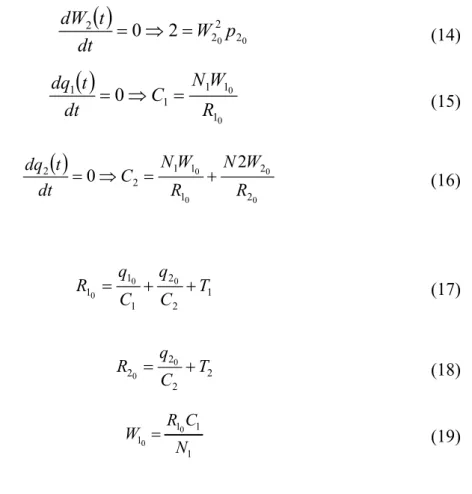
1. Efficient queue utilization: the queue should not be empty or overflown. In the first case, the link capacity is spoilt while in the second the loss of packets will cause retransmissions.
2
3. Robustness: the possible changes in the configuration of a network require AQM controllers to be able to maintain their performance in spite of variations in the number of TCP sessions, the propagation delays or the capacity of the links. There are many congestion control algorithms in the literature:
Classic approaches: RED (and its variants), REM, BLUE, YELLOW, …
Automatic control approaches: fuzzy control, robust control, predictive control, PID, adaptive PID,etc.
These approaches study in depth what happens with one congested router, even there are examples of two or more routers with problems, but, as far as the authors know, no study has been done on how the tuning of the controller can affect other routers. Although each router is considered as an individual control problem, when there are changes (number of users, flow, network capacity, etc) that affect surrounding nodes, this also alters the performance of ‘our’ router. This is a multivariable system (MIMO), there are several inputs and several outputs and the dependency between variables is not linear.
The paper will show how these changes affect routers in the neighborhood and how although working with SISO controllers, results can be very different. The paper presents a topology with two routers that can present congestion and how depending on the type of controller and the tuning method the results can be better or worse. The system is modelled as a non-linear MIMO fluid model ([1] ) . Even as we know that the system is MIMO, controllers are tuned as SISO. This can lead to several problems. The controllers we compare are:
PID for each router tuned following the Cohen-Coons tuning rules.
PID finely tuned.
Simple adaptive gain scheduling PID ([1] ).
The paper is structured as follows: section 2 describes the fluid model of a multi-bottleneck topology and the particularization to 2-routers with congestion problems. Section 3 presents different control approaches; section 4 discusses the working procedure and the simulation results. Finally conclusions and future work are presented.
2. PROBLEM SETTING
There are many variants of TCP, but the one that has been widely studied and analyzed by far is TCP/IP New Reno. This section describes the general fluid model for a network constituted by several routers and then the particular topology utilized as example in this paper.
2.1 Fluid model of a multirouter TCP/IP New Reno scenario
The dynamics of an AQM router are complex due to the number of variables that come into play: packet sources, protocols, etc. Nevertheless, it is possible to obtain a nonlinear model that represents the dynamics of the system
Let us consider a network composed by a set of routers V = {1, . . . , nv} which may
transport a set of TCP flows F = {1, . . . , nf }. Given that flows may not cross all the
routers in the network, we define the auxiliary sets Vf and Fv respectively as the set of
routers crossed by the TCP flow f∈F and the set of TCP flows which cross the router v∈V.
3
that, for simplicity, we will ignore the TCP timeout mechanism in this paper. Thus, the model is given by equations (1) and (2).
Where:
f is the number of routers.
Is the average TCP window size in packets of the TCP fϵF.
Is the average queue length (packets) of the router vϵV.
Rf is the round-trip time of the TCP flow fϵF, which is given by
Tfis the propagation delay of TCP flow fϵF(s).
is the probability of marking a packet of the f flow.
Equation (1) represents the control dynamics of the TCP window. As it can be seen, the size of the window is increased by one unit every round trip time (additive increase effect) and decreased to its half at the instant of the arrival of a loss (multiplicative decrease part). Equation (2) is the differential version of the Lindley equation and models the queue length as the accumulated difference between the packet arrival rate and the link capacity.
Figure 1. Example Topology
R
t
R
t
p
t R
t
tR t W W t R dt dW
f f f
f
f f f
f
f
ˆ
2 1
0 , ,
0 max
0 ,
v F
f f
f v
F
f f v
f v
v
q t R
t W C
q t R
t W C
dt t dq
v v
(1)
(2)
0, max
f
f W
W
0, max
v
v q
q
f
V
v v f
v
f C T
t q t
R
4
2.2 Network topology
As explained in the introduction one of the objectives of the paper is to show that there is a relevant interaction among routers and that depending on the controller and/or tuning method the congestion can be avoided or decreased its influence. In order to show this, a particular case of multi-router topology is used (Figure 1).
There are two routers (R1 and R2) where congestion can occur. Equations 3-6 and their worked out expressions 7-10 represent the non-linear behavior of the topology depicted in Figure 1.
These equations will be simulated in Matlab/Simulink® to represent the real system. The mathematical equations describing this topology are:
R
t
R
t
p
t R
t
p
t R
t
t R t W t W t R dt t dW 2 2 1 1 1 1 1 1 1 1 1 2 1
(3)
t
R
t
W
N
C
dt
t
dq
1 1 1 11
(4)
R
t
R
t
p
t R
t
t R t W t W t R dt t dW 1 2 2 2 2 2 2 2 2 2 1 (5)
R
t
t W N t R t W N C dt t dq 2 2 2 1 1 1 22
(6)
Working with them, we obtain:
()
( ) 2 ) ( 2 ) ( 12 10 10 20 1
10 2 10 2 10 1 10 2 10 1 2 10 20 10 2 10 2 1
1 p p w t
R W t R W t R W t r R p p R W dt t dW
(7)
( ) ( ) 1 2 10 10 1 1 10 11 r t
R W N t W R N dt t
dq
(8)
) ( 2 ) ( 2 ) ( 1 ) ( 2 20 2 20 2 20 2 20 2 20 1 2 20 2 20 20 20 2 t R W t r p R W t r R t w R p W dt tdW
(9)
( ) ( ) ( ) ( ) 2 2 20 20 2 1 2 10 10 1 2 20 2 1 10 12 R t
R W N t R R W N t W R N t W R N dt t
dq
(10)
where:
12 2 1 1 1 T C t q C t q t
R (11)
22 2 2 T C t q t
R (12)
With initial conditions given by:
0 0
0 1 2
2 1
1 0 2 W p p
dt t dW
5
0
0 2
2 2
2 0 2 W p
dt t
dW
(14)
0 0
1 1 1 1
1 0
R W N C dt
t
dq
(15)
0 0
0 0
2 2
1 1 1 2
2 0 2
R W N R
W N C dt
t dq
(16)
Then,
1 2 2
1 1
10 0 C0 T
q C q
R (17)
2 2 2
20 C0 T
q
R (18)
1 1 1
10 0
N C R
W (19)
2.3 One router fluid model
This subsection presents a brief description of the fluid model when only one congested router is taken into account. The non-linear model can be found in [3] and [1] among others. This model is important because it is linearized and then the transfer function that relates the queue size in packets (Q) with the probability of marking a packet (p) is obtained.
Figure 2. Dumbbell Topology
6
The two non-linear equations that define the model are:
1 ( ) ( ( ( )))
( ) ( ( ))
( ) 2 ( ( ))
( )
( ), 0
( ) ( )
( )
max 0, ( ) , 0
( )
TCP
TCP
W t W t R t R t
W t p t R t
R t R t R t
N t
C W t q
R t q t
N t
C W t q
R t
&
&
, (20)
Where:
W: average TCP window size (packets),
q: average queue length (packets), R: round-trip time = q/C+Tp (secs),
C:link capacity (packets/sec), Tp: propagation delay (secs),
NTCP: load factor (number of TCP sessions) and
p: probability of packet mark.
2.4 Classic Approach to Transfer function of one router fluid model
Linearizing the model given by equation (20) and considering only the low frequencies (nominal behavior) the following transfer function is obtained:
0 2
0 2
1 2
2
R s C R
N s
N C s
G
(21)
So, Q(s) =G(s)P(s) if working in an open loop approach. It is a second order system with no zeros and two poles that are always real. The gain is always negative and very big. This affects greatly at the coefficients of the controller: they have to be very small. The negative sign reflects the behavior of the system: the greater the probability, the smaller the queue: if more packets are discarded, the queue size will be smaller.
This transfer function will be used to tune each of the PI controllers that will regulate the queue size of each router of the proposed dumbbell topology.
The block diagram that summarizes the one router congestion control problem is shown in Figure 3. Details regarding the tuning will be given in following section.
7
2.4 Normalized Transfer function of one router fluid model
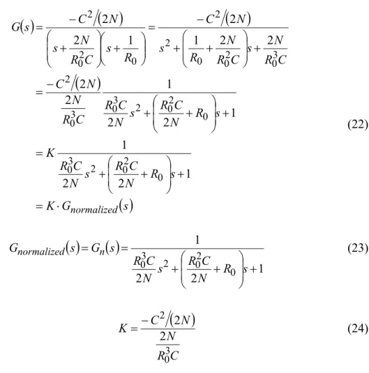
As explained in previous subsection, the system’s gain is very big and depends greatly on the number of users (N) and the link capacity (C). So, some numerical transformations are done and G(s) (equation 21) is now:
s G K s R N C R s N C R K s R N C R s N C R C R N N C C R N s C R N R s N C R s C R N s N C s G normalized 1 2 2 1 1 2 2 1 2 2 2 2 1 2 1 2 2 0 2 0 2 3 0 0 2 0 2 3 0 3 0 2 3 0 2 0 0 2 2 0 2 0 2 (22)
1 2 2 1 0 2 0 2 3 0 s R N C R s N C R s G sGnormalized n (23)
C R N N C K 3 0 2 2 2 (24)
For the sake of clarity, let’s call Gn(s) to Gnormalized(s). The PI controller will include an
adaptive gain K, that will change with the number of users and the link capacity. The block diagram that reflects this is shown in figure 4.
Figure 4. One router control system, PI adaptative gain Next section will describe how each controller has been tuned.
3. TUNING OF CONTROLLERS
We have chosen the PID controller (equation 25, [2] ) as the AQM congestion control algorithm, as it is the most common form of feedback control technique and relevant
CPI K 0 Gn(s
sR
8
results can be found in the literature regarding the stability properties and the tuning. The structure of the controller when the three terms are included: proportional, integral and derivative is:
t d p i t d
i
p et T e d T dedtt K et K e d K dedtt
K t u
0 0
1
(25)
However, the derivative term will not be used in our proposal, due to the presence of noise at high frequencies, which would be amplified by this term. Thus, the performance is better when this term is not considered in the design, so the proposed controller is a Proportional Integral (PI) controller, so Equation 25 can be further simplified to:
t p i t
i
p et T e d K et K e d
K t u
0 0
1
(26)
There are many proposed rules to tune PI controllers; for example, the parameters Kp
and Ti (or Ki) can be selected following the Cohen Coon tuning method, which is
based on estimating some parameters from the response to a step change in the control signal in manual mode and then using simple formula. In any case the two parameters frequently need some fine tuning to ensure robustness and performance at the different working points.
Following the result presented in (23, 24), it is proposed here that the PI controller include an adaptive gain K, that changes with the number of users N and the link capacity C. This makes possible to use optimal values at each combination of users N and link capacity C, which improves the performance when these parameters change, as shown in the Case Study at the end of the paper. Let’s remark that this approach only changes the proportional gain of the controller and that the integral time is the same under both PI approaches.
4. CASE STUDY
This section describes the steps that have been followed to work with the multi-router system, the tuning (exact values of the parameters) and simulation results.
The different stages have been:
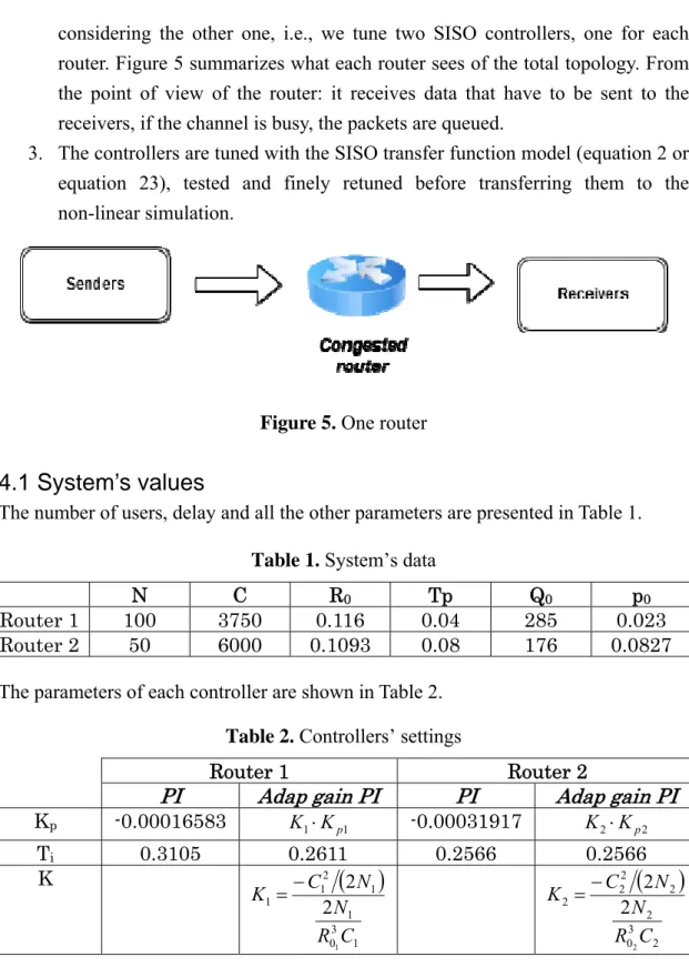
1. Simulate the non-linear model of the system showed in figure 1 and described in section 2 in Simulink©. If we were working with a real network this step would be omitted.
9
considering the other one, i.e., we tune two SISO controllers, one for each router. Figure 5 summarizes what each router sees of the total topology. From the point of view of the router: it receives data that have to be sent to the receivers, if the channel is busy, the packets are queued.
3. The controllers are tuned with the SISO transfer function model (equation 2 or equation 23), tested and finely retuned before transferring them to the non-linear simulation.
Figure 5. One router
4.1 System’s values
The number of users, delay and all the other parameters are presented in Table 1.
Table 1. System’s data
N C R0 Tp Q0 p0
Router 1 100 3750 0.116 0.04 285 0.023 Router 2 50 6000 0.1093 0.08 176 0.0827
The parameters of each controller are shown in Table 2.
Table 2. Controllers’ settings
Router 1 Router 2
PI Adap gain PI PI Adap gain PI
Kp -0.00016583 K1Kp1 -0.00031917 K2Kp2
Ti 0.3105 0.2611 0.2566 0.2566
K
1 3 0
1 1 2 1 1
1
2 2
C R
N N C
K
2 3 0
2 2 2 2 2
2
2 2
C R
N N C K
10
Figure 6. Block diagram, classic PI
Figure 7. Block diagram, adaptive gain PI
4.2. Simulation results
The experiment presented in Figures 8 to 11 correspond to the following changes in some of the router parameters:
1. At time t=10 secs the Capacity of the first router is abruptly reduced from 3750 to 3000 packets.
2. At time t=20 the Capacity of the second router is abruptly reduced from 6000 to 5400. 3. At time t=30 the Number of users of the first router is increased from 100 to 150. 4. At time t=40 the Number of users of the second router is reduced from 50 to 75. During all the experiment the designed controller aims to maintain the flow around 313 in the first router and 192 in the second router (these values are on purpose selected to be different from the nominal values, in order to test the robustness of the designed controller in different working conditions).
11
Figure 8. Predicted flow in Router 1 for the experiment of Section 4 (Blue: using varying gain PI; Purple: using constant gain PI)
Figure 9. Predicted flow in Router 2 for the experiment of Section 4 (Blue: using varying gain PI; Purple: using constant gain PI)
Figure 10. Predicted discard probability in Router 1 for the experiment of Section 4
12
5. CONCLUSIONS
A detailed analysis of the congestion control problem in the presence of multiple routers has been presented using simulation. This has made possible to compare the congestion controller proposed by the authors with PID controllers tuned using standard ideas: as variations in the gain and bandwidth are inherent to the system and interaction between routers is unavoidable the controller has to be robust.
The results are encouraging and more work is being done to show these properties also using standard network simulation software (ns2). These results justify the use of more advanced control structures that pass information between controllers of different routes in the network. This would be the subject of further work, together with the application to other congestion control schemes, such as those in [7,8].
6. ACKNOWLEDGEMENTS
The first author would like to thank funding provided by Funded by MiCInn DPI2014-54530-R and FEDER funds.
7. REFERENCES
[1] T. Alvarez and A. Salim. How to reduce congestion on TCP/AQM networks with simple adaptive PID controllers. Proceedings of the UKACC’12, 2012.
[2] K.J. Aström and T. Hägglund. Advanced PID control. ISA: NC, 2006.
[3] C. V. Hollot, Vishal Misra, Donald Towsley, and Weibo Gong. Analysis and design of controllers for AQM routers supporting TCP flows. IEEE Transactions on Automatic Control, 47(6): 945–959, June 2002.
[4] V. Jacobson. Congestion avoidance and control. ACM SIGCOMM computer communication review,18,(4): 314-329),1998.
[5] V. Misra, W. B. Gong, and D. Towsley. Fluid-based analysis of a network of AQM routers supporting TCP flows with an application to RED. ACM SIGCOMM Computer Communication Review, 30(4): 151-160, 2000.
[6] L. Wang, L. Cai, X. Liu, X. Shen and J. Zhang. Stability analysis of multiple-bottleneck networks. Computer Networks, 53: 338-352, 2009.J
[7] Jain, M., Tomar, D. S., & Singh, S. K. (2015). A Survey on TCP Congestion Control Schemes in Guided Media and Unguided Media Communication. International Journal of Computer Applications, 118(3).