Bounded Rational Formation of Beliefs:
Explaining Biased Assessment of
Probabilities in Insurance and Hedging
Markets
†
Pedro J. Guti´
errez
∗Carlos R. Palmero
∗∗University of Valladolid, Spain
Abstract
We show that, jointly withmoral hazard andadverse selection, insur-ance and hedging activities present an additional problem related to the accuracy of agents’ beliefs. In particular, we show that contrary to the market selection hypothesis, departure from accurate beliefs is, in some circumstances, beneficial for agents. To prove it, we provide a standard canonical general equilibrium model of insurance markets showing that bounded rational moderate optimistic traders with incorrect beliefs ob-tain, period by period, higher actual expected utility and higher actual expected wealth than agents with accurate beliefs. Our findings are then consistent with the empirical evidence showing a systematic and coherent optimistic bias of agents in the assessment of probabilities.
JEL classification: D51, D84, D90.
Keywords: General Equilibrium Model; Arrow-Debreu Securities; Bounded Rationality; Accuracy of Beliefs.
1
Introduction
Once uncertainty was consistently introduced into economic analysis in the early 1950s by Arrow (1953), Debreu (1953, 1959) and Savage (1952, 1954), insurance and hedging activities soon became a central issue in economic theory. As a re-sult of this interest, two important problems inherent to insurance markets were identified during the 1960s and the 1970s, namelymoral hazard andadverse se-lection. In both problems, the ultimate cause is the existence of informational asymmetries. In a moral hazard problem, the insurer is unable to determine
†Financial support from Education and Science Department, Spanish Government, research project ECO2009-10231 is gratefully acknowledged. The suggestions of Alan Kirman, Guido A. Baldi and the participants at the 1st Conference of the Herbert Simon Society noticeably improved the final outcome and are highly appreciated. The authors also acknowledge the kind assistance of A.F. Hynds.
∗Corresponding author. E-mail address: [email protected] (P.J. Guti´errez). ∗∗E-mail address: [email protected] (C. R. Palmero).
1 INTRODUCTION 2
the change in the probability of the risky event motivated by the subscription of the insurance contract1. In an adverse selection problem, the insurer
can-not differentiate between the risky and non-risky insurance buyers, therefore assigning the same probability for the risky event to all the individuals2. As
a consequence of these information asymmetries, the insurance/hedging mar-ket becomes inefficient, fails to reduce individual risks, and does not replicate the social optimum, reasons that justify the great interest in these questions in today’s economics.
In this paper, we show that together with these two well known problems, insurance and hedging markets present additional matters worth examining, directly related to the accuracy of agents’ subjective beliefs. More specifically, two questions arise regarding the rationality of agents beliefs: What are the implications of the accuracy degree in agents’ subjective beliefs?; and, Why agents continuously and consistently incur in an optimistic bias when assessing probabilities?
Indeed, these unknowns are at the core of a central puzzle in today’s eco-nomics. On the one hand, there exist strong theoretical arguments justifying the so called market selection hypothesis, without any doubt the main theoretical result concerning the relevance of accurate beliefs: In canonical models of in-surance markets, essentially Arrow-Debreu general equilibrium economies with complete markets, agents with accurate beliefs are selected by the market over those with incorrect beliefs, since they earn higher expected wealth. This mar-ket selection hypothesis, proposed by Alchian (1950), Friedman (1953), Cootner (1964) and Fama (1965) during the 1950s and 1960s, and more recently by San-droni (2000, 2005) and Blume and Easley (2006), is nevertheless contradicted by empirical evidence. As documented by Arnould and Grabowski (1981), DeJoy (1989), Camerer and Kunreuther (1989), De Long, Shleifer, Summers and Wald-mann (1990, 1991), Shleifer and Summers (1990), Palomino (1996), Alpert and Raiffa (1982), Weinstein (1980), Buehler, Griffin and Ross (1994), and Puri and Robinson (2007), there is substantial evidence revealing that agents habitually overestimate the probability of good outcomes, consistently and continuously maintain an optimistic bias in their assessment of probabilities, and can earn higher expected wealth than agents with correct beliefs by adopting biased be-liefs.
The introduction of a bounded rational mechanism of belief formation can help to solve this puzzle of paramount importance in current economic theory. To provide the intuition behind this possibility, let us consider a standard gen-eral equilibrium model of insurance markets in which insurance and hedging activities operate on the basis of the household heterogeneity condition and the law of large numbers. In simple words, it is assumed that when an agent of-fers an Arrow-Debreu security, there is another agent wishing to demand it; or, equivalently, that when a state of nature is relatively better for a household, it is simultaneously relatively worse for at least another household. Without any loss of generality to our purposes, let us assume that there exist two states of nature (1 and 2) and two households (A and B), and that state of nature 1 is the relatively better for household A and the relatively worse for household B. Therefore, there exist two Arrow-Debreu securities: Arrow-Debreu security 1,
1See Arrow (1965, 1971).
2See the seminal article by Akerloff (1970), and also Laffont (1985) and Hirshleifer and
1 INTRODUCTION 3
which provides 1 unit of good at state of nature 1, and Arrow-Debreu security 2, which provides one unit of god at state of nature 2. To hedge against risk, household A sells Arrow-Debreu security 1 and buys Arrow-Debreu security 2, whilst household B sells Arrow-Debreu security 2 and buys Arrow-Debreu security 1.
Let us consider that there does not exist social risk, that both agents are rational and have the true probabilities as beliefs, and that therefore they totally hedge against risk. From this initial situation, let us now assume that household A becomes optimistic assigning a higher probability of occurrence to his/her relatively better state3of nature 1, and therefore a lower probability to his/her relatively worse state of nature 2. As is well known, agents optimally allocate more wealth to the states of nature that they consider more likely to occur; consequently, in this general equilibrium framework, household A will sell a lower quantity of Arrow-Debreu security 1 in order to increase her/his wealth at state of nature 1, now more probable, and will buy a lower amount of Arrow-Debreu security 2 in order to decrease her/his wealth at state of nature 2, now less likely. The price of the Arrow-Debreu security 1 will then increase since the supply of Arrow-Debreu security 1 has decreased, whilst the lower demand of Arrow-Debreu security 2 will originate a fall in the Arrow-Debreu security 2 price. Obviously, these changes in prices benefit the optimistic agent A and are prejudicial to agent 2 despite his/her more accurate beliefs. Indeed, given that the now more optimistic household A sells Arrow-Debreu security 1 at a higher price and buys Arrow-Debreu security 2 at a lower price, he/she is able to increase his/her wealth at the expense of the rational agent B, who buys Arrow-Debreu security 1 at a higher price and sells Arrow-Arrow-Debreu security 2 at a lower price. This reallocation of wealth alters the initial equilibrium characterized by the total removal of uncertainty, leading to a non-efficient sharing of risk from the social point of view. From the individual perspective, however, optimism is clearly beneficial for agents, and it can be assumed therefore that there is a natural –and rational– tendency for individuals to depart from accurate beliefs and to become optimistic. Indeed, this incentive toward an optimistic change in the agents’ subjective beliefs can be understood as a mechanism of belief formation, worthy of a deeper analysis.
The first question is: How strong and how valid is this incentive to ra-tional optimism? By applying standard economic arguments, we can deduce that the success of becoming more rationally optimisticdepends on several as-pects. The first is the capability of the optimistic agent to exert influence on the Arrow-Debreu security prices. As we have seen, the benefits of optimism are a consequence of the modification in the relative price of the Arrow-Debreu security prices, a modification caused by the alteration of the individual behav-ior. If we assume competitive markets, then the only way optimism can produce an aggregate reallocation of wealth is through some kind of spreading of this sentiment. In this respect, by their nature, hedging and insurance markets are prone to experience contagion of sentiments: on the one hand, although the original underlying market can be atomized, the existence of cooperatives, mu-tual associations, and in general of big insurance and hedging companies, can lead to the concentration of buyers and sellers, opening the possibility to exert
3This intuitive formalization of optimism has been proposed, among others, by Hirshleifer
1 INTRODUCTION 4
influence on the Arrow-Debreu security prices. On the other hand, hedging and insurance markets are markets in which information and news flow very easily and quickly between agents, leading to simultaneous and concordant decisions of a big number of Arrow-Debreu security buyers or sellers, decisions that there-fore can alter the Arrow-Debreu relative prices. In this respect, we will assume throughout this paper that there exists a real possibility of optimism (and pes-simism) having influence over the Arrow-Debreu security prices, focusing on the particularities and effects of this influence.
The second aspect to consider when analyzing this incentive towardsrational optimism is its confrontation against reality. When an individual assigns a higher probability to her/his good states, she/he can get better Arrow-Debreu security prices, as we have seen. Nevertheless, if the actual probability of her/his good state is lower than his/her subjective probability, and, accordingly the true probability of his/her bad state is greater than that subjectively assigned, the real outcomes will imply more than expected bad states and fewer than expected good states. Given that the rationally optimistic agent has decided to allocate a lower wealth to her/his bad states, more probable than expected, and a greater wealth to her/his good states, less likely than expected, she/he is betting against reality and losing expected wealth. On this point and as we will show in the following sections, only when optimism is moderate the positive effects derived from the more favorable Arrow-Debreu security prices surpass the negative effects of the uncertainty misperception. Indeed, under extreme optimism, outcomes are worse than under accurate beliefs, since the costs of the distorted expectations are higher than the benefits of optimism.
Finally, there exists an important additional issue concerning the way in which the agents envisage the uncertainty scheme and formulate the objective for this change in beliefs. Both aspects are the consequence of their ability to perceive and process information and to make the associated calculations. In this respect, we will consider that these tasks are carried out by bounded rational agents, in the sense proposed by Simon (1957, 2000). More specifically and as Simon (2000) summarizes, we will assume that“the choices the people make are determined not only by some consistent overall goal and the properties of the external world, but also by the knowledge that decision makers do and don’t have of the world, their ability or inability to evoke that knowledge when it is relevant, to work out the consequences of their actions, to conjure up possible courses of action, to cope with uncertainty (including uncertainty derived from the possible responses of other actors), and to adjudicate among their many competing ways. Rationality is bounded because these abilities are severely limited.”
1 INTRODUCTION 5
of taking insurance decisions and to the non-existence of plausible explanations of insurance activities. On this point and as usual in the economic literature on insurance and hedging activities, we will assume that the considered insur-ance and hedging markets entail only stationary uncertainty. The second aspect concerning substantive rationality refers to the way the agents formulate their goals when taking decisions under uncertainty and evaluating the implications of changing their subjective beliefs, i.e. to the objective functions considered in the mechanism of belief formation. In this respect and as we will clarify in section 2, our model introduces another suggestion posed by Simon (2000) when dealing with environments with uncertainty, namely the necessity of taking into account, under a bounded rational perspective, how the involved agents react to the action of any of them.
In particular, we will assume that, for a given set of subjective beliefs con-cerning the underlying stationary scheme of uncertainty, agents maximize their logarithmic expected utility. The reason for this formulation is that expected utility maximization with logarithmic utility is an evolutionary dominant objec-tive, coherent with our procedural rationality assumption of agents consciously or unconsciously pursuing their survival. As proved by Sinn (2003), this is a dominant preference in the sense that a population following any other prefer-ence for decision-making under risk, will disappear relative to the population following this preference with a probability that approaches certainty4. It is
worth noting that this assumption does not contradict bounded rationality, since it not only incorporates two universally accepted psychophysical laws –namely Webers and Fechners Psychophysical Laws– as bounded rationality preconizes, but also implies very tractable problems under simple stationary uncertainty schemes.
Concerning the mechanism of belief formation, we will assume that the agents fix as criterion the maximization of theirone-period-ahead true expected utility. This is a logical criterion, not only heuristically reasonable but also compatible with rational decision-making individuals with limited cognitive and calculation abilities. More specifically, we will assume that each household trans-fers probability from a bad state to a good state in order to improve her/his future one-period ahead true expected utility. From the economic point of view, the election of this criterion obeys several reasons, all of them related to the paradigm of bounded rationality proposed by Simon (1957). First, it is obvious that agents do not exactly know the true probabilities of the different states of nature, and they proceed to adjust their subjective probabilities heuristically. Second, we can also admit that households continuously revise their beliefs in the light of the observed actual evidence, and, logically, this revision pursues the improvement of the real outcome that the consumer perceives. The con-sideration of the true/objective expected utility appears then as a very logical criterion for the agents, since it informs on the real gains the agent is obtaining by changing her/his beliefs. Moreover, given the usual assumption on the strict quasi-concavity of the Bernoulli logarithmic utility function, the improvement of the true/objective expected utility necessarily implies the improvement of the true/objective expected wealth/consumption, an additional objective fact that could be assessed by households when modulating their subjective beliefs,
4On the psychlogical and biological aspects of expected logarithmic utility, see also Karni
2 THE OPTIMAL EXPECTATIONS GENERAL EQUILIBRIUM 6
and that, as the former, is compatible and coherent with our assumption on the psychology of agents pursuing survival. In addition, the maximization of the one-period-ahead true expected utility is a problem the agents can tackle from the perspective of bounded rationality: given the stationarity of the uncertainty, it can be considered as a measurable and identifiable objective as time passes; and it is a simple one-period problem, whose solution (carried out consciously or unconsciously) does not entail excessive calculation abilities. Note that a completely rational agent would maximize his/her true expected utility for the total time horizon he/she is considering, a very complicated multi-period prob-lem difficult to visualize, compute and solve and that we consider to be beyond the capabilities of real households (even the abilities of expert mathematicians). Finally, as explained above and as we will clarify in the following sections, this mechanism of belief formation explicitly takes into account the reaction of an agent to the decision adopted by the remaining agents, a salient feature of bounded rationality when dealing with uncertainty according to Simon (2000). The rest of the paper is as follows. After this introduction, section 2 describes the economy -a canonical economy with insurance markets- and defines the bounded rational optimal expectations general equilibrium in the sense we have commented above. Section 3 presents the main theoretical results concerning the role played by biased beliefs, and these results are applied to some illustrative examples in section 4. Finally, section 5 concludes and provides directions for future research.
2
The Economy and its Bounded Rational
Op-timal Expectations General Equilibrium
In essence, our economy is defined by the usual assumptions in a canonical general equilibrium model of insurance/hedging markets5. More specifically, our
economy is an infinite-period exchange economy withIhouseholds, denoted by
i,i= 1,2, . . . , I, and one physical good. Lett= 0,1, . . . ,∞denote the period of time. Uncertainty is originated by the occurrence each periodtof one of a finite set of possible states of nature, characterized by a specific distribution across households of good endowments. Let Lbe the number of states of nature that can happen at any period, and letlbe each particular state,l= 1,2, . . . , L. Let us denote bySthe subsequent uncertainty/event tree; byseach node or history in the uncertainty/event tree; by sl, l = 1,2, . . . , L, the nodes immediately subsequent to s; by s−1 the node immediately preceding s; by wi(s) the
endowment of good for householdiat nodes; and byt(s) the period of time at which history/nodeshappens. Concerning the probability of occurrence of each nodes∈ S, we depart from the canonical model in considering the existence of subjective probabilities that can differ from the objective/true probabilities. On this point, let π(s) andπ1(s) be, respectively, the objective and the subjective
probabilities of occurrence for nodes. Therefore, assuming stationary stochastic processes, for any node/historys∈ S, s:= (s−t(s), s−t(s) + 1, . . . , s−1, s),
π(s) =π(s|s−1)π(s−1|s−2). . . π(s−t(s) + 1|s−t(s))π(s−t(s)),
5The reader can find the basis of the theory of insurance markets in Laffont (1989) and
2 THE OPTIMAL EXPECTATIONS GENERAL EQUILIBRIUM 7
πi(s) =πi(s|s−1)πi(s−1|s−2). . . πi(s−t(s) + 1|s−t(s))πi(s−t(s)).
Insurance/hedging activities operate on the basis of a complete system of Arrow-Debreu securities, in which all the consumers competitively trade. At each node
s ∈ S, there existL possible states of nature with respect to the next period
t(s) + 1, and therefore L Arrow-Debreu securities. We will denote by aisl the amount bought (if positive) or sold (if negative) by householdi of the Arrow-Debreu security l providing one unit of good if state of naturel happens after nodesand 0 units otherwise, and byqsl the price of this Arrow-Debreu security
l.
From the methodological point of view, the main characteristic of our model is the definition of the general equilibrium through a double maximization con-dition. In a first step and as usual, agents maximize their discounted expected utility given their respective subjective beliefs. In a second step, they choose the optimal subjective probabilities in order to maximize their real one-period-ahead expected utility. Our approach therefore follows the idea ofoptimal ex-pectations posed by Brunnermeier and Parker (2005), but with two distinctive features. First, we conclude the existence of benefits from bounded rational optimism through the analysis of the general equilibrium solution objective properties, perfectly observable, and not from the introduction of an additional function maximized by each agent. Second, in our model, agents consistently and continuously keep presenting biased optimistic beliefs because they get, at the next period, a higher actual expected utility and a higher actual expected wealth. These are objective criteria ensuring a systematic and consistent bias in the assessment of probabilities, different and alternative from that proposed by Brunnermeier and Parker (2005), and closer to the idea of bounded rationality. Indeed, in Brunnermeier and Parker (2005), the mechanism of belief forma-tion is based on the improvement, under optimism, of a well-being funcforma-tion defined as an average of real and subjective utilities. This well-being function is defined as the expected time-average of the felicity of the agent, a mix of real historical and future subjective expected utilities6. This implies that the
problem that the households must solve in Brunnermeier and Parker (2005) in order to calculate their optimal expectations, involves not only the maximiza-tion in the subjective probabilities of an infinite-period problem, but also to do so across repeated realizations of uncertainty, actually a very complicated problem demanding a huge capacity and ability of idealization and calculation. Our proposal is, in this respect, much more simple and concordant with the real abilities of real households, since it entails the maximization in the sub-jective probabilities of a one-period function, namely the one-period-ahead true expected utility, a relatively easygoing problem and much easier to visualize by the households. Our mechanism of belief formation is not only closer to the idea of bounded rationality and the real capabilities of households, but also provides a complete explanation of why agents with bounded rational optimal expecta-tions are not driven out of the market by agents with accurate beliefs. Indeed, in Brunnermeier and Parker (2005) there is no formal analysis of the evolutionary consequences of their results, whilst in our model, agents with bounded rational optimism survive in the economy because they earn more expected wealth than agents with accurate beliefs. In any case, our optimal expectations approach joins and complements that proposed by Brunnermeier and Parker (2005) and
2 THE OPTIMAL EXPECTATIONS GENERAL EQUILIBRIUM 8
adds to the literature identifying theoretical arguments implying the consistent persistence of incorrect optimistic beliefs7.
Summing up and to clarify concepts, we will define the optimal expectations general equilibrium in two steps. In a first stage we will impose the usual general equilibrium conditions, so the I households will maximize their expected dis-counted utility given their respective subjective beliefs, and markets will clear. In a second step, we will consider that the consumers choose the subjective beliefs/probabilities that maximize their future one-period-ahead true expected utility, something which ensures the improvement of their one-period-ahead true expected wealth. Therefore, in this second step, the consumers will fix their sub-jective beliefs as those beliefs that make their one-period ahead true expected utility maxima and improve their true expected wealth when the economy is in a general equilibrium consistent with their subjective beliefs.
2.1
Subjective General Equilibrium
Let us consider the problem solved by each household in our economy,
maxCi s,aisl
P s∈Sβ
t(s)
i πi(s)Ui(Csi)
s.t. Ci s+
PL l=1qsla
i
sl≤wi(s) +ais
Ci s≥0
s∈ S
(1)
where βi, Ui and Csi are, respectively, the time discount factor; the Bernoulli
utility function; and the consumption at nodesfor householdi. Under the usual assumptions (U(·) increasing and strictly quasiconcave), the former problem has solutions in Ci
s and aisl, which depend on the whole set of Arrow-Debreu
security prices and on the whole set of subjective probabilities, that is, on qsl
and πi(s), where s∈ S and l = 1,2, . . . , L. Letq and πi be, respectively, the sets q:={qsl|s∈ S, l= 1,2, . . . , L} andπi :={πi(s)|s∈ S}. We will therefore
denote the solution functions byCsi(q, πi) andaisl(q, π
i). These functions must
also verify the market equilibrium conditions
PI i=1C
i
s(q, πi) = PI
i=1w
i(s),
PI i=1a
i sl(q, π
i) = 0,
s∈ S, l= 1,2, . . . , L,
(2)
and then the subjective general equilibrium is defined as:
Definition 1 (Subjective General Equilibrium) Set of functionsCˆi s(q, πi)
andˆai sl(q, π
i),s∈ S,l= 1,2, . . . , L,i= 1,2, . . . , I, and set of pricesqˆ
sl,s∈ S,
l = 1,2, . . . , L, solving the household’s problems (1) and verifying the market clearing conditions (2).
7See De long, Shleifer, Summers and Waldmann (1990, 1991), Shleifer and Summmers
2 THE OPTIMAL EXPECTATIONS GENERAL EQUILIBRIUM 9
2.2
Bounded Rational Optimal Expectations Equilibrium
Under the canonical assumptions –increasing and strictly quasiconcave Bernoulli utility functions and strictly positive endowments– the former subjective general equilibrium exists, and leads to the equilibrium prices of the Arrow-Debreu securities. For each Arrow-Debreu security, its equilibrium price depends on the subjective probabilities of all the households, and therefore so do the general equilibrium optimal consumptions. Let πSE be the set of all the subjective probabilities, i.e. πSE := {πi|i = 1,2, . . . , I}. Then, the solution functionsdefining the subjective general equilibrium are ˆCi
s(πSE) and ˆaisl(π
SE), s ∈ S,
l= 1,2, . . . , L,i= 1,2, . . . , I.
Let us now consider as reference any node s and its immediately subse-quent nodessl,l= 1,2, . . . , L. In our framework of insurance/hedging markets, materialized in the existence at node s of a complete set of L Arrow-Debreu securities, households trade in these Arrow-Debreu securities to transfer wealth across states of nature. Therefore, at node s, each household will sell Arrow-Debreu securitylif nodeslis arelatively good node, and will buy Arrow-Debreu securitylif nodeslis arelatively bad node. Consequently,ai
sl <0 if nodeslis a
relatively good node, andaisl >0 if nodesl is arelatively bad node. Letπi(sl|s) be the subjective beliefs of household i at node s concerning nodes sl. Ac-cording to our reasonings, when household i becomes more optimistic, she/he transfers subjective probability from her/his relatively bad states to her/his relatively good states, causing a favorable alteration in the relative price of the associated Arrow-Debreu securities –determined in the subjective general equilibrium– through changes in the Arrow-Debreu supplies and demands. As a consequence, there also appear changes in the solution allocation defining the subjective general equilibrium, and the question to elucidate is then when these changes are beneficial for the optimistic agent. In other words, since in the subjective general equilibrium the final allocation depends on the set of all the subjective beliefs, it is possible for each consumer to modify in her/his own benefit the equilibrium solutions by modulating her/his subjective probabilities. In this respect and as we explained above, we will assume that each house-hold transfers probability from a bad state to a good state in order to improve her/his future one-period-ahead true expected utility at the subjective general equilibrium. In this respect, let Es[Ui( ˆCi)] denote, at nodes, the household
i true expected one-period-ahead utility at the subjective general equilibrium, i.e.
Es[Ui( ˆCi)] =π(s1|s)Ui( ˆCsi1) +π(s2|s)U
i( ˆCi
s2) +. . .+π(sL|s)U
i( ˆCi sL).
The preceding ideas led to the following definition:
Definition 2 (Bounded Rational Optimal Expectations General Equilibrium) An optimal expectations general equilibrium is a set of functions Cˆsi(q, πi) and
ˆ
ai sl(q, π
i), a set of pricesqˆ
sl, and a set of subjective probabilitiesˆπi(sl|s),s∈ S,
l= 1,2, . . . , L,i= 1,2, . . . , I, such that
• Cˆi
s(q, πi),ˆaisl(q, πi), andqˆsl,s∈ S,l= 1,2, . . . , L, constitute a subjective
general equilibrium, and
• ˆπi(sl|s)solve the household’s problems
max
πi(sl|s)Es[U
3 THEORETICAL RESULTS 10
On the basis of this definition of optimal expectations general equilibrium, we will provide in the following section some useful mathematical results ensuring the existence of bounded rational moderate optimism of agents in insurance and hedging markets. In addition, we will numerically and/or algebraically solve four canonical general equilibrium models of insurance markets, showing how their optimal expectations general equilibrium imply the presence of a bounded rational optimistic bias in beliefs, which in addition are evolutionary compatible.
3
Theoretical Results
By their nature, in general and with very few exceptions, the class of general equilibrium models of insurance/hedging markets that we have considered do not have an algebraic solution, and must be numerically solved. This incon-venience forces us to prove the existence of optimism in agents by making use of very simple models with algebraic solutions, or alternatively, by ensuring the verification of simple mathematical properties in the optimal expectations general equilibrium solutions. In the following lines we present three set of suf-ficient conditions, easily testable, which ensure and/or prove the existence of a bounded rational bias in the optimal expectations equilibrium. As we will show in section 4, these conditions are verified by all the standard models of insurance markets with algebraic solution.
Given nodesand household i, let us subdivide the set of theL immediate subsequent nodes/states into two subsets, namely the subsetGi
sof the household
i relatively good states, and the subset Bi
s of the household i relatively bad
states. Taking into account the sign of the householdi Arrow-Debreu security holdings, these sets are defined as follow:
Gis:={l∈L|aisl<0}, Bis:={l∈L|aisl>0}.
Obviously, for householdi, the total true probabilities of being at a good state or at a bad state, respectively Π(Gis) and Π(Bsi), are given by
Π(Gis) = X
l∈Gi s
π(sl|s), Π(Bsi) = X
l∈Bi s
π(sl|s).
Let ˆCi Gi
s and ˆC
i Bi
s be the set of the subjective general equilibrium optimal
con-sumptions at the good and bad states, respectively
ˆ
CGis :={Cˆsli|l∈Gis}, CˆBis :={Cˆsli|l∈Bis}.
From the definitions of the two aggregate true probabilities Π(Gi
s) and Π(Bis)
and of the sets ˆCGii s and ˆC
i Bi
s, the household itrue expected one-period ahead
utility at the subjective general equilibriumEs[Ui( ˆCi)] can be written
Es[Ui( ˆCi)] = Π(Gis)V( ˆC i Gi
s) + Π(B
i s)W( ˆC
i Bi
s),
where
V( ˆCGii s) =
P l∈Gi
sπ(l|s)U
i( ˆCi sl)
Π(Gi s)
3 THEORETICAL RESULTS 11
W( ˆCBii s) =
P l∈Bi
sπ(l|s)U
i( ˆCi sl)
Π(Bi s)
.
Let us now consider any good state/node g ∈ Gis and any bad state/node
b ∈ Bsi. Let us assume that household i increases πi(sg|s) in detriment of
πi(sb|s), becoming more optimistic. Since the subjective general equilibrium
optimal consumptions ˆCi
sl depend on the subjective probabilities, so do the
functions V( ˆCi Gi
s) and W( ˆC
i Bi
s), and then a change dEs[U
i( ˆCi)] in the
one-period ahead true expected utility appears. This change is given by
dEs[Ui( ˆCi)] = Π(Gis)[
∂V( ˆCGii s)
∂πi(sg|s)dπ
i(sg|s) +∂V( ˆC i Gi
s)
∂πi(sb|s)dπ
i(sb|s)]+
Π(Bsi)[
∂W( ˆCi Gi
s)
∂πi(sg|s)dπ
i(sg|s) +∂W( ˆC i Gi
s)
∂πi(sb|s)dπ i(sb|s)].
Sincedπi(sg|s) =−dπi(sb|s)>0,
dEs[Ui( ˆCi)] =
(
Π(Gis)[∂V( ˆC
i Gi
s)
∂πi(sg|s)−
∂V( ˆCGii s)
∂πi(sb|s)] + Π(B i s)[
∂W( ˆCGii s)
∂πi(sg|s) −
∂W( ˆCGii s)
∂πi(sb|s) )
dπi(sg|s)],
and then
dEs[Ui( ˆCi)]>0⇔
(
Π(Gis)[
∂V( ˆCi Gi
s)
∂πi(sg|s)−
∂V( ˆCi Gi
s)
∂πi(sb|s)] + Π(B i s)[
∂W( ˆCi Gi
s)
∂πi(sg|s) −
∂W( ˆCi Gi
s)
∂πi(sb|s) )
>0.
• Sufficient Conditions 1: Let us assume thatV( ˆCi Gi
s) is increasing and
concave in πi(sg|s) and decreasing and concave in πi(sb|s), and that
W( ˆCi Bi
s) is increasing and concave inπ
i(sb|s) and decreasing and concave
inπi(sg|s). Then, if∀i
∂V( ˆCi
Gis)
∂πi(sg|s)−
∂V( ˆCi
Gis)
∂πi(sb|s)
∂W( ˆCi Gis)
∂πi(sb|s) −
∂W( ˆCi Gis)
∂πi(sg|s)
πi(sg|s)=π(sg|s)
>Π(B
i s)
Π(Gi s)
,
all the households are optimistic at the bounded rational optimal expec-tations general equilibrium.
Proof The proof is immediate by applying basic arguments of algebra and calculus. 2
• Sufficient Conditions 2: Letπi
s= (πi(s1|s), . . . , πi(sL|s)),i= 1, . . . , I.
Let us assume that the optimal consumption functions at the subjective general equilibrium ˆCi
sl(π
SE), s ∈ S, l = 1,2, . . . , L, are concave in πi s.
3 THEORETICAL RESULTS 12
a) If
∂Es[Ui( ˆCi]
∂πi(sl|s)
πi(sl|s)=π(sl|s)
>0
for some i= 1, . . . , I, and some l = 1, . . . , L, the bounded rational optimal expectation equilibrium implies non-accurate biased beliefs.
b) If∀i
∂Es[Ui( ˆCi]
∂πi(sl|s)
πi(sl|s)=π(sl|s)
>0 ∀l∈Gis,
and
∂Es[Ui( ˆCi]
∂πi(sl|s)
πi(sl|s)=π(sl|s)
<0 ∀l∈Bis,
the bounded rational optimal expectation equilibrium implies biased optimistic beliefs for all the agents.
Proof Let πSE
s be the vector of the subjective probabilities assigned at
nodes∈ Sto the occurrence of the different states of the world at the following period for all households, i.e. πSE
s := (πs1, . . . , πsi, . . . , πIs)∈IR
I×L, whereπi s=
(πi(s1|s), . . . , πi(sL|s)) for alli = 1, . . . , I. Let π
s be the vector, at node s ∈
S, of the true probabilities of occurrence of the different states of nature, i.e.
πs := (π(s1|s), . . . , π(sL|s)). As we know, the solution functions defining the
subjective general equilibrium are ˆCi
s(πSE) and ˆaisl(πSE),s∈ S,l= 1,2, . . . , L,
i= 1,2, . . . , I. At any nodes∈ S, the one-period-ahead true expected utility associated to the subjective general equilibrium is given by the expression
Es[Ui( ˆCi)] =
π(s1|s)Ui( ˆCsi1(πSE)) +π(s2|s)Ui( ˆCsi2(πSE)) +. . .+π(sL|s)Ui( ˆCsLi (πSE)).
At each nodes∈ S, let us now consider the game in which each householdi
is described by her/his one-period-ahead true expected utility at the subjective general equilibrium Es[Ui( ˆCi] and by his/her set of available actions, namely
her/his set of subjective probabilities, defined by
Ai={πis= (πi(s1|s), . . . , πi(sL|s))∈IR L
:πi(sl|s)∈[0,1]∀l= 1, . . . , L}.
The cartesian product A = A1× · · · ×AI is the action space of the game,
and an element of A is a vector πSEs := (πs1, . . . , πsi, . . . , πsI) ∈ IRI×L, which specifies the subjective probabilities chosen by all agents. The actions of all agents jointly determine the result of this game in the form of a payoff to each agent,Es[Ui( ˆCi],i= 1, . . . , I, which depends on both her/his actions and those
of all the other agents.
In order to establish the existence of a Nash equilibrium for the game in normal form Γ = ((Es[Ui( ˆCi], Ai) : i= 1, . . . , I), it suffices to show that the
game satisfies the following conditions of Nash’s Theorem:
(i) For eachi= 1, . . . , I, the payoff functionEs[Ui( ˆCi] :A−→IR is
continu-ous and quasi-concave inπSE
s := (π1s, . . . , πis, . . . , πIs)∈IR
I×L, for a given
πsSE−i:= (π1s, . . . , πsi−1, πis+1, . . . , πIs)∈IR
(I−1)×L
,
3 THEORETICAL RESULTS 13
(ii) For each i = 1, . . . , I, the action space Ai is a nonempty, compact, and
convex subset of IRL.
First, notice that Ai is a compact and convex subset of IRL. Next, consider
the payoff function for agent i, Es[Ui( ˆCi]. Since each composite function
Ui( ˆCi
sl(πSE)) is concave inA (this is becauseUi is an increasing and concave
function, and ˆCi
sl is assumed to be concave inπsi), and any nonnegative linear
combination of concave functions is a concave function, Es[Ui( ˆCi] is concave
and therefore quasi-concave. Thus, the conditions of Nash’s Theorem are satis-fied, and it follows that the game has one Nash equilibriumπs?= (π1
?
s , . . . , πL
?
s )
in A, which means that it is a feasible action (i.e. π?s ∈ A) and it is the best
response to the joint actions of all the other agents, that is
¯
πsi?∈arg max
πi s∈Ai
Es[Ui( ˆCi(πsi, π SE−i?
s ).
Hence, given that the rest of the agents playπSEs −i?, there is no incentive for the
ith agent to deviate unilaterally from the equilibrium actionπis?, or equivalently,
for alli= 1, . . . , I,πsi? is a solution for the problem
max
πi s∈Ai
Es[Ui( ˆCi(πsi, π SE−i?
s )], (3)
where the actionsπsSE−i? chosen by the other agents are given.
For our purposes, we are interested in knowing the properties of the Nash equilibrium with respect to the accuracy of the households beliefs. In partic-ular, we would like to know if the optimal probabilities π?
s coincide with the
true probabilitiesπs, or, on the contrary, if the Nash equilibrium πs? implies a
departure from accurate beliefs.
In this sense, we will prove that, under a very weak assumption which is satisfied in practice, then π?
s 6=πs, and the true probability πs is not a Nash
equilibrium, contradicting themarket selection hypothesis. To do this, we con-sider the following result for a nonlinear maximization problem with nonnegative constraints:
Ifπsi? is an optimal solution for problem (3), then
it follows that ∂Es[Ui( ˆCi]
∂πi(sl|s) (πi ?
s , πSE−i
?
s )≤0 for alll= 1, . . . , L.
Thus, whenever ∂Es[Ui( ˆCi]
∂πi(sl|s) (πs)>0 for somei= 1, . . . , I, and somel= 1, . . . , L,
the true probability profile πs will not be a Nash equilibrium, and therefore
π?s6=πsand part a) is proved.
To prove part b), it is enough to consider the sign of the partial derivatives
∂Es[Ui( ˆCi]
∂πi(sl|s)
πi(sl|s)=π(sl|s)
>0 ∀l∈Gis,
and
∂Es[Ui( ˆCi]
∂πi(sl|s)
πi(sl|s)=π(sl|s)
<0 ∀l∈Bsi,
4 PARTICULAR CASES 14
4
Particular Cases
4.1
Model 1
Let us consider the simplest canonical model of insurance markets. The economy is a one-period exchange economy with two households, denoted by A and B, and one physical good. Uncertainty is originated by the occurrence at the unique period of one of two possible states of nature, characterized by a specific distribution across households of good endowments. On this point, letl = 1,2 be the states of nature, and let wA
l and w B
l be the endowments at node l of
householdAandB, respectively. Without any loss of generality, we will assume that state of naturel= 1 is the relatively good state for householdA, and that state of nature l = 2 is the relatively good state for household B. Therefore
wA
1 > wA2 andwB2 > w1B. On the basis of this uncertainty scheme, households
trade in two Arrow-Debreu securities with real pricesq1 andq2.
Let the Bernoulli utility function of the two households beU(C) = ln(C). The subjective general equilibrium is therefore defined as follows:
Definition 3 (Subjective General Equilibrium) Set of functionsCˆlA(q1, q2, π1A, π
A
2),
ˆ
ClB(q1, q2, πB1, πB2), ˆaAl (q1, q2, π1A, πA2) and ˆaBl (q1, q2, π1B, π2B), and set of prices
ˆ
ql,l= 1,2, solving the household’s problems
maxCA l,aAl π
A
1 ln(C1A) + (1−πA1) ln(C2A)
s.t. q1aA1 +q2aA2 = 0
CA
1 =wA1 +aA1
CA
2 =wA2 +aA2
CA
1, C2A≥0
,
maxCB l ,a
B l π
B
1 ln(C1B) + (1−π1B) ln(C2B)
s.t. q1aB1 +q2aB2 = 0
C1B=wB1 +aB1
CB
2 =wB2 +aB2
CB
1 , C2B ≥0
,
and verifying the market clearing conditions
C1A+C1B=wA1 +wB1, C2A+C2B=wA2 +wB2,
aA1 +aB1 = 0, aA2 +aB2 = 0.
This subjective general equilibrium has an algebraic solution, given by the following functions:
ˆ
C1A(π1A, q1, q2) =
πA
1(q1wA1 +q2wA2)
q1
, Cˆ2A(π1A, q1, q2) =
(1−πA
1)(q1wA1 +q2w2A)
q2
4 PARTICULAR CASES 15
ˆ
C1B(πB1, q1, q2) =
πB
1(q1w1B+q2w2B)
q1
, Cˆ2B(π1B, q1, q2) =
(1−πB
1)(q1w1B+q2w2B)
q2
,
ˆ
aA1(π1A, q1, q2) = ˆC1A(π
A
1, q1, q2)−wA1, ˆa
A
2(π
A
1, q1, q2) = ˆC2A(π
A
1, q1, q2)−w2A,
ˆ
aB1(πB1, q1, q2) = ˆC1B(πB1, q1, q2)−wB1, ˆaB2(πB1, q1, q2) = ˆC2B(πB1, q1, q2)−wB2,
ˆ
q1=π1Aw2A+π1BwB2, qˆ2= (1−π1A)wA1 + (1−π1B)wB1.
After substituting the equilibrium prices ˆq1and ˆq2into the optimal
consump-tions, we get the subjective general equilibrium consumptions as a function of the whole set of subjective beliefs and endowments:
ˆ
C1A(π1A, πB1) =
πA
1[πB1(wA1wB2 −w1BwA2) +wA2(w1a+wB1)]
πA
1wA2 +πB1w2B
,
ˆ
C2A(πA1, π1B) =
(1−π1A)[π1B(wA1w2B−wB1w2A) +w2A(wa1+wB1)]
(1−πA
1)wA1 + (1−π1B)wB1
,
ˆ
C1B(πA1, π1B) =π
B
1[(1−πA1)(wA1w2B−w1Bw2A) +w1B(wa2+w2B)]
πA
1w2A+π1BwB2
,
ˆ
C2B(πA1, π1B) = (1−π
B
1)[(1−πA1)(w1AwB2 −w1Bw2A) +wB1(w2a+wB2)]
(1−πA
1)w1A+ (1−πB1)wB1
.
It is immediate to prove that ˆCA
1 is increasing and concave inπA1, and that
ˆ
CA
2 is decreasing and concave inπA1. We can apply the set of sufficient conditions
1 since the optimal expectations general equilibrium problem
max
πA
1
E[ln( ˆCA)] =π1ln( ˆC1A(π
A
1, π
B
1) + (1−π1) ln( ˆC2A(π
A
1, π
B
1)
has a unique interior solution, given by the reaction function
ˆ
π1A(π1B, π1 ) =
p
πB1wB2
2[π(πB
1(w1AwB2 −w1BwA2) +w1BwA2) +wB1wA2(πB1 −1)]
[wb1(1−πB1)p[4π1 (πB1)(wa1wB2 −wB1wA2) +wA2(wA1 +wB1)−4π21∗(πB1 ∗(wA1wB2 −wB1wA2) + (wa2(wa1+wB1)))−πB1wB1wB2(πB1 −1)]+ p
πB1wB2(2∗πB1w1A−w1B(πB1 −1))] and
∂E[ln( ˆCA)]
∂πA 1 πA
1=π1
>0⇔ w
A
1wB2
wB
1w2A
> π1(1−π
B
1)
πB
1(1−π1)
.
Therefore, the last inequality provides a necessary and sufficient condition ensur-ing the bounded rational optimism of household A, i.e. ensuring that ˆπA
1 > π1.
By applying the same arguments to householdB, when the inequality
∂E[ln( ˆCA)]
∂(1−πB
1) πB
1=π1
>0⇔ w
A
1w2B
wB
1wA2
>π
A
1(1−π1)
π1(1−πA1)
,
holds, household B is necessarily bounded rational optimistic and 1−πˆB
1 >
4 PARTICULAR CASES 16
The questions to elucidate are then, first, whether the optimal expectations general equilibrium can imply the existence of optimism for both agents; and second, whether this bounded rational optimistic departure from accurate beliefs has a limit. With respect to the first question, it is enough to show that the second set of sufficient conditions holds, or, equivalently, that the two above inequalities are compatible when there exist insurance markets. Since, when
πA
1 =π1B=π1, we get
wA1w2B
wB
1wA2
>1 = π
A
1(1−π1)
π1(1−π1A)
= π1(1−π
B
1)
πB
1(1−π1)
,
then
∂E[ln( ˆCA)]
∂πA
1
πA
1=π1
>0, ∂E[ln( ˆC
A)]
∂(1−πB
1)
πB
1=π1
>0,
∂E[ln( ˆCA)]
∂(1−πA
1)
πA
1=π1
<0, ∂E[ln( ˆC
A)]
∂πB
1
πB
1=π1
<0,
and the second set of sufficient conditions is verified. Therefore, at the bounded rational optimal expectations equilibrium, both agents are bounded rational optimistic agents.
Alternatively, let us assume that wA1w2B wB
1wA2
>1 and that there exist insurance
markets. Since π1A(1−π1) π1(1−π1A)
is continuous and increasing in πA, and π1(1−πB1) πB
1(1−π1) is continuous and decreasing in πB, given that when πA = π and πB =π both fractions are equal to 1, there always existπB < πandπA> π for which
wA
1wB2
wB
1w2A
> π1(1−π
B
1)
πB
1(1−π1)
and
wA
1wB2
wB
1w2A
>π
A
1(1−π1)
π1(1−π1A)
.
Concerning the second question, it is obvious that the reaction functions ˆ
πA1(π1B, π1) and ˆπ1B(πA1, π1) provide the values above which optimism is
4 PARTICULAR CASES 17
Table 1. Model 1.
π1 = 0.5;π2 = 0.5;wA1 =wB2 = 120;wA2 =wB1 = 80.
Moderate Extreme True expected True expected True expected
πB1 πAˆ1 optimism optimism utility and consumption utility and consumption utility and consumption of agent A, optimal of agent A, accurate of agent B, optimal
optimism of agent A beliefs of agent A optimism of agent A
0.45 0.56 [0.5,0.56] (0.56,1] 4.60001 4.59629 4.598150
100.092013 99.2430 99.90798
0.5 0.58 [0.5,0.58] (0.58,1] 4.61164876 4.60517019 4.59209226
100.971455 100 99.0285448
0.6 0.6 [0.5,0.6] (0.6,1] 4.6443909 4.62941936 4.56434819
104 102.950311 96
Nash Equilibrium.
πA?1 πB?2 πA?2 πB?1 True Expected True Expected (optimistic) (optimistic) (optimistic) (optimistic) Utility and Consumption, Utility and Consumption,
Nash equilibrium accurate beliefs
0.5505 0.5505 0.4495 0.4495 4.60004349 4.60517019
100 100
4.2
Model 2
Let us now consider the simplest dynamic canonical model of insurance markets. The economy is a two-period exchange economy with two households, denoted byAandB, and one physical good. Uncertainty is originated by the occurrence at the second period of one of two possible states of nature, characterized by a specific distribution across households of good endowments. Let s = 0,1,2 denote, respectively, the initial state of nature and the two possible future nodes at periodt= 1, and letwA
s andwsB be the endowments at nodesof households
A and B, respectively. Without any loss of generality, we will assume that node/state of natures= 1 is the relatively good state for householdA, and that state of nature s = 2 is the relatively good state for household B. Therefore
wA
1 > wA2 andwB2 > w1B. On the basis of this uncertainty scheme, households
trade in two Arrow-Debreu securities with real pricesq1 andq2.
Let the Bernoulli utility function of the two households beU(C) = ln(C), and let the time discount factor β be the same for the two households. The subjective general equilibrium is therefore defined as follows:
Definition 4 (Subjective General Equilibrium) Set of functionsCˆsA(q1, q2, π1A),
ˆ
CB
4 PARTICULAR CASES 18
andl= 1,2, solving the household’s problems
maxCA
s,aAl ln(C
A
0) +β[πA1 ln(C1A) + (1−π1A) ln(C2A)]
s.t. CA
0 +q1aA1 +q2aA2 ≤wA0
C1A=wA1 +aA1
CA
2 =wA2 +aA2
CA
0, C1A, C2A≥0
,
maxCB
s,aBl ln(C
B
0) +β[π1Bln(C1B) + (1−π1B) ln(C2B)]
s.t. CB
0 +q1aB1 +q2aB2 ≤w0B
C1B=wB1 +aB1
CB
2 =wB2 +aB2
CB
0, C1B, C2B ≥0
,
and verifying the market clearing conditions
C0A+C0B=wA0 +wB0, C1A+C1B =w1A+w1B, C2A+C2B=wA2 +wB2,
aA1 +aB1 = 0, aA2 +aB2 = 0.
This subjective general equilibrium has an algebraic solution, given by the following functions:
ˆ
C0A(π1A, q1, q2) =
wA
0 +q1w1A+q2wA2)
1 +β) ,
ˆ
C1A(π1A, q1, q2) =
βπA
1(wA0 +q1w1A+q2wA2)
q1(1 +β)
,
ˆ
C2A(π
A
1, q1, q2) =
β(1−πA
1)(w0A+q1wA1 +q2w2A)
q2(1 +β)
,
ˆ
C0B(π1B, q1, q2) =
w0B+q1w1B+q2wB2)
(1 +β) ,
ˆ
C1B(π1B, q1, q2) =
βπ1B(wB0 +q1wB1 +q2wB2)
q1(1 +β)
,
ˆ
C2B(πB1, q1, q2) =
β(1−π1B)(w0B+q1w1B+q2w2B)
q2(1 +β)
,
ˆ
aA1(π
A
1, q1, q2) = ˆC1A(π
A
1, q1, q2)−wA1, ˆa
A
2(π
A
1, q1, q2) = ˆC2A(π
A
1, q1, q2)−w2A,
ˆ
aB1(πB1, q1, q2) = ˆC1B(π
B
1, q1, q2)−wB1, ˆa
B
2(π
B
1, q1, q2) = ˆC2B(π
B
1, q1, q2)−wB2,
ˆ
q1 =
β[β(wA0 +wB0)(πA1wA2 +πB1wB2) + (wA2 +wB2)(πA1wA0 +πB1wB0)] (wA
1 +wB1)(wA2 +wB2)−β[πA1(wA1wB2 −wB1wA2) +πB1(wB1wA2 −wA1wB2)−(wA1 +wB1)(wA2 +wB2)]
4 PARTICULAR CASES 19
ˆ
q2 =
β[β(wA0 +wB0)((1−πA1)wA1 + (1−πB1)wB1) + (wA1 +wB1)((1−πA1)wA0 + (1−πB1)wB0)]
β[πA1(wA1wB2 −wB1wA2) +πB1(wB1wA2 −wA1wB2)−(wA1 +wB1)(wA2 +wB2)]−(wA1 +wB1)(wA2 +wB2)
.
After substituting the equilibrium prices ˆq1and ˆq2into the optimal
consump-tions, we get the subjective general equilibrium consumptions as a function of the whole set of subjective beliefs and endowments:
ˆ
CA0(πA1, πB1) =
β(wA0 +wB0)[πB1(wA1wB2 −wB1wA2) +wA2(wA1 +wB1)] +wA0(wA1 +wB1)(wA2 +wB2) (wA1 +wB1)(wA2 +wB2)−β[πA1(wa1wB2 −wB1wA2) +πB1(wB1wA2 −wA1wB2)−(wA1 +wB1)(wA2 +wB2)]
,
ˆ
CB0(π1A, π1B) =
β(wA
0 +wB0)[πA1(wA1wB2 −wB1wA2)−wB2(wA1 +wB1)]−wB0(wA1 +wB1)(wA2 +wB2)
β[πA
1(wa1wB2 −wB1wA2) +πB1(wB1wA2 −wA1wB2)−(wA1 +wB1)(wA2 +wB2)]−(wA1 +wB1)(wA2 +wB2)
,
ˆ
CA1(πA1, πB1) =
πA
1[β(wA0 +wB0)(πB1(wA1wB2 −wB1wA2) +wA2(wA1 +wB1)) +wA0(wA1 +wB1)(wA2 +wB2)]
β(wA
0 +wB0)(πA1wA2 +πB1wB2) + (wA2 +wB2)(πA1wA0 +πB1wB0)
,
ˆ
CB1(π1A, πB1) =
πB
1[wA0(wA1 +wB1)(wA2 +wB2)−β(wA0 +wB0)(πA1(wA1wB2 −wB1wA2)−wB2(wA1 +wB1))]
β(wA0 +wB0)(πA1wA2 +πB1wB2) + (wA2 +wB2)(πA1wA0 +πB1wB0)
,
ˆ
CA2(πA1, πB1) = (πA
1 −1)[β(wA0 +wB0)(πB1(wA1wB2 −wB1wA2) +wA2(wA1 +wB1)) +wA0(wA1 +wB1)(wA2 +wB2)]
β(wA0 +wB0)((πA1 −1)wA1 + (πB1 −1)wB1) + (wA1 +wB1)((πA1 −1)wA0 + (πB1 −1)wB0)
,
ˆ
CB2(π1A, π1B) =
(1−πB1)[β(wA0 +wB0)(πA1(wA1wB2 −wB1wA2)−wB2(wA1 +wB1))−wA0(wA1 +wB1)(wA2 +wB2)]
β(wA0 +wB0)((πA1 −1)wA1 + (πB1 −1)wB1) + (wA1 +wB1)((πA1 −1)wA0 + (πB1 −1)wB0)
.
It is immediate to prove that ˆCA
1 is increasing and concave inπA1, and that
ˆ
CA
2 is decreasing and concave inπA1. The bounded rational optimal expectations
general equilibrium problem
max
πA
1
E[ln( ˆCA)] =π1ln( ˆC1A(π
A
1, π
B
1) + (1−π1) ln( ˆC2A(π
A
1, π
B
1)
has a unique interior solution8. Given that
(w
A
1w
B
2
wB1w2A >
π1(1−π1B)
π1B(1−π1)
)∧(π1B≤π1+
π1
2β)∧( w1AwA2 wB1wB2 ≥
πB1(1 + 2β)−2βπ1
π1(1 + 2β)−2βπB1
)⇒
∂E[ln( ˆCA)]
∂πA 1 πA
1=π1
>0,
we can apply the first set of sufficient conditions to ensure the presence of bounded rational optimism for householdA, i.e. to ensure that ˆπA
1 > π1.
By applying the same arguments to householdB, when the set of inequalities
(w A 1w B 2 wB 1w A 2 >π A
1(1−π1)
π1(1−π1A)
)∧π1A≤π1+
π1
2β)∧( w1Aw2A wB
1w
B
2
≥ π1(1 + 2β)−2βπ
A
1
πA
1(1 + 2β)−2βπ1
)
holds, household B is necessarily bounded rational optimistic and 1−πˆB
1 >
1−π1.
As in the previous model, the questions to elucidate are the same: first, whether this bounded rational optimistic departure from accurate beliefs has a limit; and second, whether the bounded rational optimal expectations gen-eral equilibrium can imply the existence of bounded rational optimism for both agents. In this respect, we reach the same conclusions as in the previous case by applying the same reasonings. The reader can carry out similar analyses for the
8We do not provide this solution/reaction function given its large expression. The
4 PARTICULAR CASES 20
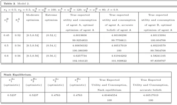
second set of sufficient conditions, and can obtain the conditions under which these results are verified. In table 2 we provide some numerical results showing that moderate optimism is beneficial, extreme optimism is prejudicial, and that there exist optimal expectations equilibria implying bounded rational moderate optimism for both agents. Again, the Nash Equilibrium does not replicate the social optimum and entails the inefficient appearance of macroeconomic risk.
Table 2. Model 2.
π1 = 0.5;π2 = 0.5;wA0 =wB0 = 100;wA1 =wB2 = 120;wA2 =wB1 = 80;β= 0.9.
Moderate Extreme True expected True expected True expected
πB1 πAˆ1 optimism optimism utility and consumption utility and consumption utility and consumption of agent A, optimal of agent A, accurate of agent B, optimal
optimism of agent A beliefs of agent A optimism of agent A
0.45 0.52 [0.5,0.52] (0.52,1] 4.6019606 4.60166296 4.60115094
99.9254853 99.7758811 100.004768
0.5 0.54 [0.5,0.54] (0.54,1] 4.60656332 4.60517019 4.60216579
100.380389 100 99.7804768
0.6 0.56 [0.5,0.56] (0.56,1] 4.6257734 4.61944202 4.58241105
102.164123 101.938822 97.8358767
Nash Equilibrium.
πA?1 πB?2 πA?2 πB?1 True Expected True Expected (optimistic) (optimistic) (optimistic) (optimistic) Utility and Consumption, Utility and Consumption,
Nash equilibrium accurate beliefs
0.5237 0.5237 0.4763 0.4763 4.60404554 4.60517019
100 100
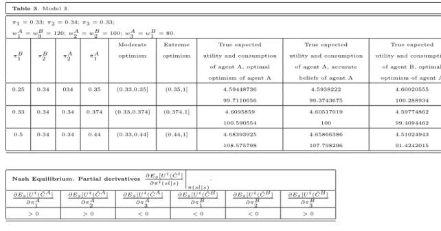
4.3
Model 3
Let us now consider the simplest canonical model of insurance markets when the number of states of nature is greater than 2. The economy is a one period exchange economy with two households, denoted byAandB, and one physical good. Uncertainty is originated by the occurrence at the unique period of one of three possible states of nature, characterized by a specific distribution across households of good endowments. On this point, let l = 1,2,3 be the states of nature, and letwA
l andw B
l be the endowments at nodelof householdAandB,
respectively. Without any loss of generality, we will assume that state of nature
l = 1 is a relatively good state for householdA, that state of nature l = 3 is a relatively good state for household B. Therefore, for householdA, wA
1 ≥wA2
and wA
1 > w3A, or wA1 > wA2 and wA1 ≥ wA3. Analogously, for household B,
wB
3 > w1B and w3B ≥wB2, or wB3 ≥wB1 and w3B > wB2 . On the basis of this
uncertainty scheme, households trade in three Arrow-Debreu securities with real prices q1,q2 andq3.
Let the Bernoulli utility function of the two households beU(C) = ln(C). The subjective general equilibrium is therefore defined as follows:
Definition 5 (Subjective General Equilibrium) Set of functionsCˆA
l (q1, q2, π1A, πA2),
ˆ
CB
4 PARTICULAR CASES 21
ˆ
ql,l= 1,2,3, solving the household’s problems
maxCA l,a
A l π
A
1 ln(C1A) +π2Aln(C2A) + (1−π1A−π2A) ln(C3A)
s.t. q1aA1 +q2aA2 +q3aA3 = 0
C1A=wA1 +aA1
CA
2 =wA2 +aA2
CA
3 =wA3 +aA3
CA
1, C2A, C3A≥0
,
maxCB l ,a
B l π
B
1 ln(C1B) +πB2 ln(C2B) + (1−πB1 −π3B) ln(C3B)
s.t. q1aB1 +q2aB2 +q3aB3 = 0
C1B=wB1 +aB1
CB
2 =wB2 +aB2
CB
3 =wB3 +aB3
CB
1, C2B, C3B ≥0
,
and verifying the market clearing conditions
C1A+C1B=wA1 +wB1, C2A+C2B =w2A+w2B, C3A+C3B=wA3 +wB3,
aA1 +aB1 = 0, aA2 +aB2 = 0, aA3 +aB3 = 0.
This subjective general equilibrium has an algebraic solution, given by the following functions:
ˆ
C1A(π1A, πA2, q1, q2, q3) =
πA
1(q1w1A+q2wA2 +q3w3A)
q1
,
ˆ
C1B(π1B, π2B, q1, q2, q3) =
πB
1(q1wB1 +q2wB2 +q3wB3)
q1
,
ˆ
C2A(πA1, π2A, q1, q2, q3) =
πA
2(q1wB1 +q2wB2 +q3wA3)
q2
,
ˆ
C2B(π1B, π2B, q1, q2, q3) =
π2B(q1wB1 +q2wB2 +q3wB3)
q2
,
ˆ
C3A(π1A, πA2, q1, q2, q3) =
(1−πA
1 −πA2)(q1wA1 +q2w2A+q3wA3)
q3
,
ˆ
C1B(πB1, πB2, q1, q2, q3) =
(1−π1B−πB2)(q1w1B+q2w2B+q3w3B)
q3
,
ˆ
aA1(πA1, π2A, q1, q2, q3) = ˆC1A(π
A
1, π
A