SPECTRAL WAVEGUIDE FINITE ELEMENTS
PACS REFERENCE :43.20 Mv
Peplow, Andrew ; Finnveden, Svante
Marcus Wallenberg Laboratory for Sound and Vibration Research Department of Vehicle Engineering
KTH
Stockholm S 100 44 Sweden
Tel. +46 8 7908017 Fax. +46 8 7906122
Email. [email protected] [email protected]
ABSTRACT
A spectral element method is described which enables reduced wave equation problems defined in regular, arbitrary length regions to be solved as a set of coupled problems over neighbouring domains. A combination of trial functions are considered, namely the specific eigenfunctions of a differential operator and a set of hierarchical polynomials. The coefficients in the representation of the acoustic pressure are obtained by imposing continuity across element interfaces and including the given boundary conditions and sources. Accurate approximations are obtained for computations of local perturbations of the ambient fluid and a study of an optimal non-reflecting boundary is discussed.
INTRODUCTION
A variational formulation for the two--dimensional Helmholtz equation in an acoustic waveguide is presented. The objective is to calculate sound transmission through local perturbations located either within the fluid or at the fluid boundary. The case considered is that of wave propagation from a monofrequency point source in a waveguide that is assumed to be straight and arbitrarily long with uniform rectangular cross--section. Characterisation of an absorbing boundary is modelled by a locally reacting impedance condition. Parameters governing the fluid wavespeed are also allowed to vary along the longitudinal direction of the waveguide. The proposed approach can provide accurate solutions over domains of arbitrary length in a certain direction; namely, an infinite waveguide solution, a semi--infinite waveguide solution and a solution within a finite rectangular region.
leads to systems of equations with a large number of degrees of freedom. Whereas, for acoustic waveguide problems a judicious choice of basis functions, which have an underlying global nature, may lead to significantly less number of degrees of freedom. For the new spectral element method presented here the basis functions inherently possess some of the wave nature of the acoustic field. Consequently, for acoustic problems posed for a waveguide geometry the spectral methods require considerably less degrees of freedom than the discrete methods.
The spectral finite element method (SFEM) applied to waveguide problems, referenced in [ 1 ] – [ 3 ] can be viewed as a merger of the dynamic stiffness method and the finite element method. Specifically the method is based on a variational formulation for non-conservative motion in the frequency domain. The SFEM has been used to study vibration in beam frame--works [ 1 ], beam--stiffened railway cars [ 2 ] and for fluid-filled pipes [ 3 ]. Finnveden used the spectral pipe elements for various cases from assessment of approximate theory, [ 4 ], to experimental SEA calculations, [ 4 ]. Use of a variational formulation for the spectral method provides a natural basis for approximations and a simple tool for combination with standard finite elements. In the following spectral finite elements are combined to solve a waveguide problem, and in particular a possible optimal local boundary condition is presented that approximates the true non-local boundary condition at an interface for a half-space. Optimal local boundary conditions have been discussed comprehensively by Givoli in [ 5 ] and [ 6 ], the ideas used here differ in that a reflection coefficient is minimised for almost all angles for all plane-wave incidence.
FINITE ELEMENT SOLUTION
In acoustic waveguides with constant cross--section the solutions of the equations of motion, {\it i.e.} Helmholtz equation, are exponential terms describing wave propagation in an axial direction with corresponding cross--sectional modes. Polynomials are derived using a procedure developed by Finnveden in [ 3 ] to describe fluid motion in the cross--section of pipe structures. The hierarchical polynomials appear in the trial functions used in the approximation for acoustic pressure,
( , )
( )
( )
N
p
x z
z
x
∧
=
g
B p
(1.1)where
g z
j( )
=
z
j−1is thej
th entry in the vectorg
( ) , 0
z
≤ ≤
z
h
. The polynomials are non-dimensionalised so that the variableξ
=
z h
/
appears in the definitions of the approximating functions.x
z
Inserting the approximating functions into a variational formulation for the Helmholtz equation, see [ 7 ] for details , evaluating certain derivatives and integrals in the z-direction, one obtains an expression for the dynamic stiffness matrices :
2
0
( )
( )
h
T T
z
z dz
r= -
ò
K
B
g
g
B
(1.2)(
)
2 0 0 0 0( )
( )
( )
( )
( )
( )
(0)
(0)
h h T
T T T
T T T
h
d
z
d
z
k
z
z dz
dz
dz
dz
ik
h
h
r r
r z z
=
ò
-ò
g
g
K
B
g
g
B
B
B +
B
g
g
-
g
g
B
(1.3)
assuming an absorbing condition at the upper and lower boundaries. After a little matrix algebra a system, (
N
´N
), of second order differential equations for the unknown functionÙ
p
follows2
2 2 0
0
x
Ù Ù ¶ + = ¶p
K
K p
(1.4) Since the system of equations (1.4) has constant matrix coefficients the solution may be written in the form( )
x
e
i xlÙ =
p
X
(1.5) whereX
is a vector representing wave amplitudes and λ wavenumbers determined by a suitable matrix eigenvalue problem. Using the definition for propagating waves in (1.5) and polynomials in the z-direction it is possible to form an appropriate trial or wave influence function over a finite axial length -L
£x
£L
.Non-reflecting boundary condition
The application of the spectral finite element method on unbounded exterior domains involves a domain decomposition of the exterior region. On an entirely artificial boundary at
z
=0
, it is possible to prescribe artificial boundary conditions (ABC) that approximate the exact non-local boundary condition, [ 5 ] and [ 6 ].Consider a plane wave
P
incincident on the boundaryz
=0
at angle θ from the normal. Writing the addition of the incoming and scattered waves as
( cos sin ) ( cos sin )
ik z x ik z x
inc ref M
P
P
P
e
q+ qR e
- q+ q=
+
=
+
(1.6)it is possible to associate the reflection coefficient with a generalised
M
thlocal boundary condition atz
=0
as, , 0
M
i j i j
i j
P
P
a
z
=x z
=
å
. (1.7)It is also possible to recover the reflection coefficient
R
0from the zero-order or rc
boundary condition, (a
0,0=ik
), and after a little manipulation the well-known expression for the reflection coefficient is obtained,0
cos
1
cos
1
R
q
q
-=
Now, reformulating the generalized boundary condition (1.7) into a form in which the general reflection coefficient may be established:
2 4 6
2,0 4,0 6,0
2 4 6
2,0 4,0 6,0
cos
sin
sin
sin
... 1
( )
cos
sin
sin
sin
... 1
M
a
a
a
R
a
a
a
q
q
q
q
q
q
q
q
q
+
+
+
+
-=
+
+
+
+
+
. (1.9)Minimizing
R
M( )
q under a suitable norm it is possible to find rational values for the unknowncoefficients
a
i j, . In turn the resulting coefficients in equation (1.7) may be incorporated into the finite element model (1.2) and (1.3). The following two examples give some sense of the scope of the method for a waveguide with varying density and a simple exterior problem.RESULTS
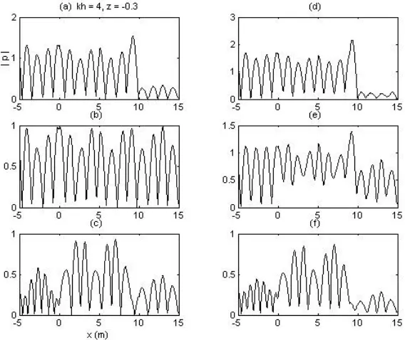
Density variation
In this example the Helmholtz equation is solved for an infinite waveguide with dimension
0.5
z
0.5
m
- £ £ including a rigid boundary where the density of the fluid is allowed to vary from ambient state r
1.21
k g m
-3 [image:4.596.116.400.430.669.2]= over the region,
9
£x
£10
m
to the right of the source. Absorbent material also covers the upper and lower boundaries of the inhomogeneous region and the source is located at the lower boundary(
0, 0.5
-)
at fixed frequency excitation 220 Hz. Figure 2 shows the absolute pressure along the waveguide just below the centre line at z = -0.3. The left hand figures (a)-(c) show pressure variation for a total rigid waveguide and the right hand figures, (d)-(f) show variation in density with absorbing material.Figure 2. Rigid waveguide (a) ñ
= 0.21 kg m
-3(b)
ñ= 1.21 kg m
-3(c)
ñ= 10.21 kg m
-3and
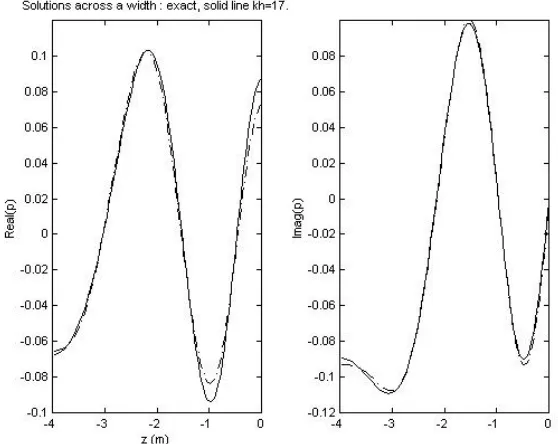
An optimal boundary condition
As a simple example to validate the high order, local,non-reflecting boundary condition above a point source was located at a rigid boundary x=0m and z = -4m in an acoustic half-space. By the method of images the exact solution is a sum of two Hankel functions of the first kind of zero order. For the numerical solution two waveguide layers were assembled with a depth of 2m each. Furthermore three coefficients, including the zero order coefficient
0,0
,
2,01
,
4,01
2
8
a
=ik a
=a
= -, (1.10)
[image:5.596.101.380.244.466.2]were incorporated into the spectral finite element solution via equation (1.3). Figure 3 shows good agreement between the analytic and numerical solutions across the waveguide domain for non-dimensional wavenumber
kh
=
17
at x=3m.Figure 3. Real and imaginary parts of finite element solution (dash-dot) to acoustic half-space problem versus the analytic solution (solid).
BIBLIOGRAPHY
1. S. Finnveden 1994, Acta Acustica 2 461-482. Exact spectral finite element analysis of stationary vibrations in a rail way car structure.
2. S. Finnveden 1996 Acustica / Acta Acustica 82 478-497. Spectral finite element analysis of stationary vibrations in a beam - plate structure.
3. S. Finnveden 1997 Journal of Sound and Vibration 199, 125-154. Spectral finite element analysis of the vibration of straight fluid-filled pipes with flanges.
4. S. Finnveden 1997 Journal of Sound and Vibration 208, 685-703. Simplified equations of motion for the radial-axial vibrations of fluid filled pipes.
5. D. Givoli 1991 J. of Computational Physics 94, 1-29. Non-reflecting boundary conditions. 6. D. Givoli 2000 Applied Numerical Mathematics 33, 327-340. Stability and accuracy of optimal local non-reflecting boundary conditions.