A NEW COMBINED METHOD FOR ROOM ACOUSTICS SIMULATION

(1)

A NEW COMBINED METHOD FOR ROOM ACOUSTICS SIMULATION

REFERENCIA PACS: 43.55.Ka

D. Alarcão; J. L. Bento Coelho CAPS-Instituto Superior Técnico P-1049-001 Lisbon, Portugal

Tel. +351 21 841-9367, Fax +351 21 846-5303 [email protected]

ABSTRACT: A new combined method for the solution of the problem of the propagation of sound energy inside arbitrarily shaped enclosures is presented. The boundaries of the modelled enclosures are composed of reflecting surfaces, which reflect the sound energy as a mixture of specular and diffuse components. This new combined method uses a mirror image source method (MISM) with statistical extensions and a time-dependent hierarchical radiosity method (TDHRM). The MISM solves for the propagation of the specularly reflected energy components, while the TDHRM solves for the propagation of the diffusely reflected energy components. Both methods operate independently from each other. The simulated room impulse response is obtained from the combination of the results yielded by each method. New algorithmic refinements are introduced in the computer implementation of this combined method. In order to validate the new combined method, a series of acoustical measurements based on the Maximum Length Sequences technique (MLS) were conducted in different rooms, ranging from small meeting rooms to medium-sized auditoriums. Simulation results and comparisons with real measurements will be shown.

INTRODUCTION

The prediction of sound fields inside arbitrary enclosures is a difficult task, but for most practical purposes in room acoustics simulations, it is sufficient to model only the propagation of sound energy inside the enclosures.

A usual approach in order to model the complex reflections of surfaces is to consider that a fraction of the energy incident on the surface is reflected specularly while the remaining fraction is diffusely reflected. In this paper we will show that if the diffusivity factor of the walls is either small for a certain group of walls or near one for another group of walls, then a combined method can be applied for solving the underlying equations. The combined method solves separately the determination of the specularly reflected components and the determination of the lambertian reflected components by using an extended image source method and a hierarchical radiosity based method [3, 4].

THEORETICAL DEVELOPMENT

In reference [1] it was shown that an equation of motion could be set up for the temporal evolution of the acoustic angular power flux over the walls of an arbitrary enclosure M:

0

( , , , ) ( , , , ) ( , , , 0)

k

Source k

i k i k j i

j

t t

β

ω

β

ω

₋

β

ω

=

∑

+

s Ω j s Ω s Ω

T T

k

(1)

where and where the integral transport and reflection operator is defined through the relation:

1 1 2 ...

k k k

(2)

(

)

[

]

(

)

( ) ( , )

( ( , ))

( , , , )

( ( , ), , , ) ( , ) ( , ), , , ( )

n

i n

m

R dt i

dt

e ω W_ττ d

β ω τ

ω − − β ⊥

+

+ =

⎡ϒ − → ⎤

⎣ ⎦

∫

' s sΩ s ' '

s s sΩ

sΩ

s sΩ Ω Ω M s s Ω s s s Ω Ω σ Ω

2 M

M M M

H

T

ω τ (2)

s

is a point located over the enclosure’s boundary,

Ω Ω

,

'are direction vectors, ω is the sound frequency and ϒ_R(s s_M( , ),Ω −Ω Ω, ', )

ω

is the so-called Wall Reflection Function, which gives the ratio between the acoustic angular power flux in the outgoing direction

−Ω

and the acoustic power flux in the incident direction . The function determines the first point of the boundary that is visible from

s

in the direction .

'

Ω

s s

_M

( ,

Ω

)

Ω

[

( , )

]

n

dt

Wτ +τ s sM Ω →s gives the transition amplitude that acoustic angular power flux is exchanged from the surface point to the surface point during the time interval comprised between

( ,

)

s s

_M

Ω

s

τ

and

τ

+dt_n. The exponential factor in (2) accounts for the air attenuation, and the integration is done over the hemisphere where the integral is to be taken in the Lebesgue sense, where the Lebesgue measure

(s ( ,s Ω))

2 M

H

( )

dσ Ω⊥_s ' stands for projected solid angle (which includes the normal cosine factor).

Therefore, given that the initial incident acoustic angular power flux is completely known at each surface point of the enclosure and for each direction

Ω

, one can then calculate the time evolution of the flux for any ulterior time instant. In analogy with dynamics, we can term equation (1) as a general equation of motion for the sound energy propagation inside enclosures.

M

Some simplifying assumptions are introduced in the following, so that a practical method for solving equation (1) can be obtained. This simplification is mainly introduced in the functional form of the Wall Reflection Function, more precisely, one will consider only functions of the form:

( , , , ) ( , , ) ( , , ) ( ( ))

R o i

ω

ρ

D i

ω

ρ

S i

ω δ

σ⊥ i M o

ϒ s Ω Ω = s Ω + s Ω Ω − _n Ω (3)

In this definition, the specular direction function is introduced, which gives the mirror direction, obtained by reflecting around the surface normal . Algebraically, this mirror direction is defined by . In addition, a special Dirac distribution

( o

M_n Ω )

o −

i o

Ω

n

( o) 2( o )

M_n Ω = Ω n n Ω

δ

_σ⊥is

introduced, which is defined by the property that

( )

(

))

( )

(

)

f

δ

_σ⊥

d

⊥

−

=

∫

'

s s

Ω

Ω Ω

σ Ω

f

Ω

'

2

H

(4)

for any function

f

that is continuous at . This notion of a Dirac distribution is slightly more general than the one usually encountered, extending the standard notion to integration on more general domains. Finally, two functions dependent only on the spatial variable

s

and on the incident direction for every frequency

'

Ω

i

Ω

ω

are also introduced in the definition (3). These are

( , , )

D i

ρ

s Ω

ω

and

ρ

_S( ,s Ω_i, )

ω

, which respectively denote the pure diffuse reflection component and the scalar multiplicator of the ideal specular reflection component.

In order to fulfil energy conservation principles [1] one adopts a surface diffusivity coefficient ( ) [0,1]ω

(3)

(

)

( ,

, )

( ,

, )

( ,

, )

( ,

, )

1 ( ,

, )

( ,

, )

i

D i i

S i i i

R

ω

ρ

ω

π

ρ

ω

≡ ∆

≡ − ∆

s

Ω

s

Ω

s

Ω

s

Ω

s

Ω

s

Ω

H

ω

(5)

and the adopted simplified form for the WSFs is therefore equal to

(

)

( , , )

( , , , ) ( , , ) i 1 ( , , ) ( , , ) ( ( ))

R o i i i i i o

R

R _σ M

ω

ω ω ω ω δ

π ⊥

ϒ s Ω Ω = ∆ sΩ H s Ω + − ∆ sΩ sΩ Ω − _n Ω

H

(6)

where

( )

( ,

_i

, )

_R

( ,

_o

,

_i

, )

(

)

R

ω

=

∫

ϒ

Ω Ω

ω

d

⊥_s

Ω

s

Ω

s

σ

_o

2

H

(7)

stands for the directional-hemispherical surface reflectivity, which is a dimensionless quantity obeying 0≤RH( ,sΩi, )ω <1, and expressing the ratio between the acoustic radiosity over the hemi-sphere H and the incoming acoustic power flux at

s

from direction

Ω

i.

By using this form for the Wall Reflection Function, the reflection and transport operator T can be split into two linear operators, one that accounts for the diffuse reflection character and another for the specular reflection character:

D S

T = T + T

(8)

where

(

)

[

]

(

)

( ) ( , ) ( ( , ))

( , , ,

)

(

( ,

),

, )

(

( ,

),

, )

(

)

( ,

)

( ,

),

, ,

n

D i n

m dt i

dt

R

e

d

W

ω τ τ

β

ω τ

ω

π

β

ω τ

− − ⊥ +

+

=

⎡

⎤

∆

×

⎢

⎥

⎢

⎥

→

⎢

⎥

⎣

⎦

∫

'

s sΩ s '

' s '

s sΩ

s

Ω

s s

Ω Ω

s s

Ω Ω

σ Ω

s s

Ω

s

s s

Ω Ω

M 2 M H M M H M M

T

(9) and

(

)

(

)

[

]

₍

₎

( ) ( , ) ( ( , )) ( , , , )

1 ( ( , ), , ) ( ( , ), , ) ( ( ))

( )

( , ) ( , ), , ,

n

S i n

m dt i dt R M d e W σ ω τ τ

β

ω τ

ω

ω δ

β

ω τ

⊥ ⊥ − − + + = ⎡ − ∆ − − ×⎤ ⎢ ⎥ ⎢ → ⎥ ⎣ ⎦

∫

' ' ' n _' s

s sΩ s '

s sΩ

s Ω

s s Ω Ω s s Ω Ω Ω Ω

σ Ω s s Ω s s s Ω Ω

M 2

M

M H M

H M M

T

(10)

By replacing (8) into the equation of motion (1) yields:

(

)

(

)

0

( , , , )

( , , ,

)

( , , , 0)

k

k Source

i k D S i k j D S i

j

t

β

ω

β

ω

₋

β

ω

=

∑

+

s

Ω

T

j

s

Ω

T

s

Ω

(11)

and expanding by using the well-known binomial formula

0 0 0

( , , , )

( , , ,

)

( , , , 0)

j

k k

m j m Source m k m

i k D S i k j D S i

j m m

j

k

t

m

β

ω

−

β

ω

−

β

ω

− = = =

⎛ ⎞

=

_{⎜ ⎟}

+

_{⎜ ⎟}

⎝ ⎠

∑∑

∑

s

Ω

T T

s

Ω

T T

s

Ω

(11)

Equation (11) shows the effect of the multiple applications of both operators

T

_Dand upon the initial flux distribution. This equation thus portrays all the intervening reflection sequences. For example, all specular-specular reflection sequences are considered, as well as all diffuse-diffuse reflection sequences, and all mixed specular-diffuse-diffuse and diffuse-diffuse-specular reflection

S

(4)

If one assumes that the values of the diffusivity coefficients are rather small in a certain part of the enclosure, denoted by

M

_Low, and near one in another part of the enclosure, denoted by

High

M

, then only the “linear” terms of the sums in equation (11) are of considerable magnitude. In this case, one can simplify equation (11) and write:

0 0

( , , , )

( , , , ) ( , , , ) ( , , , 0) ( , , , 0)

i k

k k

j Source j Source k k

D i k j S i k j D i S i

j j

t

t t

β

ω

β

ω

₋

β

ω

₋

β

ω

β

= =

=

+ + +

∑

sΩ

sΩ s Ω s Ω s Ω

T T T T

ω

Low

igh

= ∅

m k m−

(12)

provided that the conditions on the diffusivity coefficient are respected. These can be more exactly defined as

( ,

, )

1:

( ,

, )

1:

i

i H

ω

∆

∈

∆

≈

∈

s

Ω

s

Ω

s

M

(13)

where it is required that the whole enclosure’s boundary is uniquely subdivided such that

;

Low

∪

High Low

∩

High

M = M

M

(14)

In fact, let’s one analyse a general “crossed” term of the sums in equation (10), namely the term . Since in region

D S

T T

M

Lowthe diffusivity coefficients are small, meaning that ∆( ,sΩi, )ω ≤ε for all the frequencies

ω

, with

ε

1, then the multiple integrals in (10) contain a factor of order

, except in the case

(1 ) 0

ε

m −

ε

k m− ≈

ε

m≈ _m=₀

, which corresponds exactly to the term 0 k k

D S =

T T TS , i.e. a non-crossed term.

Therefore, for , the contribution of the corresponding integral will be very small. On the other hand, in region

0

m≠

High

M

one has that ∆( ,s Ω_i, )

ω

≥

ζ

with ζ = −1 γ and γ 1 for all frequencies of interest, and the contained factors are therefore of order

, except in the case

(1 ) (1 ) 0

m k m k m k m

ζ

₋

ζ

− _{≈ −}

ζ

− ₌

γ

− _≈

0

k− =m , which obviously corresponds to the non-crossed term k 0 k

D S = D

T T T . Therefore, one can see that under the assumption (13) and (14), all “crossed” terms of the binomial developments contribute negligibly to the acoustic angular power flux.

One therefore establishes the conditions of validity of the simplified formula (12), which simply states that the motion of the energy flux inside this enclosure can be determined by solving independently for the diffuse operator equations and for the specular operator equations. One can thus arrive at the basis description for a combined method for determining the sound energy propagation inside enclosures which comply to the conditions (13) and (14).

• Solving the Specular Operator Equation

Due to the specular nature of the reflection factor, translated by the normalized Dirac distribution, the only contributions to the specular operator (10) must come from directions such as given by the well known Snell-Descartes Law stating that the outgoing polar angle must be equal to the incident polar angle and that the outgoing direction must be contained in the plane of incidence. Therefore, one solution method for the specular operator equation can be achieved by the usage of an extended image source method.

• Solving the Diffuse Operator Equation

To solve the diffuse operator equation (9), one assumes that the diffusivity coefficient does not depend on the incident direction, i.e. we have that ∆( ,s Ωi, )

ω

= ∆( , )s

ω

, meaning that the

directional-hemispherical surface reflectivity depends only on the location of the surface point :

s

( , _i, ) ( , )

(5)

(

)

[

]

(

)

( ) ( , ) ( ( , ))

( , , ,

)

(

( ,

), )

(

( ,

), )

( ,

)

( ,

),

, ,

(

)

n

D i n

m dt i

dt

R

e

W

d

ω τ τ

β

ω τ

ω

π

β

ω τ

− − + ⊥

+

=

∆

→

⎡

⎤

⎣

⎦

∫

s sΩ s

' '

s s sΩ

s

Ω

s s

Ω

s s

Ω

s s

Ω

s

s s

Ω Ω

σ Ω

M 2 M H M M M M H

T

×

(15)

By integrating expression (15) over the hemi-sphere of incident directions, and introducing the definition of the incident sound power per unit area,

φ

,

(

)

[

]

(

)

( ) ( , ) ( )

(

( ,

), )

(

( ,

), )

( , ,

)

( )

( ,

)

( ,

), ,

n m D n dt

R

e

dt

d

W

ω τ τ

ω

π

φ

ω τ

φ

ω τ

− − ⊥ +

⎡

_∆

_×

⎤

⎢

⎥

+

=

_⎢

_⎥

→

⎢

⎥

⎣

⎦

∫

s sΩ s s s

s s

Ω

s s

Ω

s

σ Ω

s s

Ω

s

s s

Ω

M 2 H M M H M M

T

(16)

By introducing a local angular parameterisation, expression (16) is rewritten as

(

)

(

)

'

( )

2

( , ,

)

( , )

cos cos

( , )

, ,

( , )

( )

n D n m dt

dt

R

e

ω

W

_ττ

vis

d

φ

ω τ

ω

θ

ω

φ

ω τ

π

− − +

+

=

⎡

⎤

⎢

∆

⎡

_⎣

→

⎤

_⎦

⎥

⎢

₋

⎥

⎣

⎦

∫

' _{s s}'

' ' '

'

s

σ

s

H M

T

θ

_{s s}

' '

M

M M

(17)

where the surface point s' =s s( ,Ω)= +s d ( ,s Ω Ω) . The angle

θ

refers to the angle between the normal vector n s( ) and the direction s s− ', while the angle θ'_{equals the angle between the}

normal vector n s( )' and the direction s s− '. In addition, the visibility function that can take the binary values zero or one is introduced. The value zero corresponds to the situation when both points

s

and are occluded by some surface of the enclosure and the value one corresponds to the situation when both points and are visible to each other. This visibility function is introduced to cope with non-convex enclosures.

( , ) vis s s' '

s

_s

'

Equation (17) can be solved by using a finite element approach by discretising the enclosure’s boundary into a certain number of “patches”. A “patch” means a certain portion of a specific wall. Therefore, walls are subdivided into a certain finite number of surfaces, which we call “patches” in accordance with the usual sense as given in Radiative Transfer or Illumination Engineering [2]. Over this discretisation, a Galerkin Method with constant basis functions is employed and the resulting discretised equations can be put in the following final form [1]:

( )

(

)

' 2 ( ) , 1 ( , , ) cos cos , ₁ ( , ) ( , ) , , ( , ) ( ) ( ) j i i j D i M

m d P P j i

j i

j j j

j i P P

i j j i

P

d P P

P R P e P

c P

vis d d

ω

φ

ω τ

θ

π

ω

−

φ

ω τ

= = ⎡ ⎡ _× ⎤⎤ ⎛ ⎞ ⎢ ⎢ ⎥⎥ − ∆ ⎜ − ⎟ ⎢ _⎜ _⎟⎢ ⎥⎥ ⎢ ⎝ ⎠⎢ ⎥⎥ ⎢ ⎣ ⎦⎥ ⎣ ⎦

∑

∫∫ ∫∫

s s

s s σ s σ s H

T

(18)

(

)

'

2

1 cos cos

( ,

)

( )

i j

i j i j j

i P P _j _i

F P

P

vis

d

P

θ

π

→

=

−

∫∫∫∫

s s

σ

s

σ

s

i

(19)

is the form factor between patch P_i andP_j [4]. THE NEW COMBINED METHOD

As shown above, under certain simplifying assumptions, a new combined method was developed that allows the solution of the sound energy propagation inside enclosures with arbitrary geometries. The simplifying assumptions are:

(6)

2. The walls of the enclosure are either highly specularly reflecting or highly diffusingly reflecting. 3. For solving the diffuse operator equation, the enclosure’s boundary is subdivided into a finite number of “patches”, over which the relevant quantities are considered constant over each patch. This means that a finite basis approach is used, where the basis functions are piecewise constant functions.

The combined method then consists of independently solving for the specularly reflected sound components and for the diffusely reflected sound components. The only “bridge” between the specular and the diffuse operator is given by the diffusivity coefficients of the walls. The two energy impulse responses, specular and diffuse, can then be finally added in order to obtain the complete energy impulse response of the enclosure.

IMPLEMENTATION

The combined method was implemented in a computer program [1, 2].

The algorithm for solving the specular reflected components was implemented using an extended image source method, while the algorithm for solving the diffusely reflected components is based on a Hierarchical Radiosity [3] algorithm that allows the error thresholds to be defined by the user in order to guarantee maximum accuracy of the solution and low computation times.

RESULTS

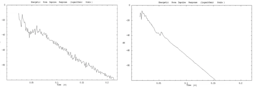
[image:6.595.90.498.443.589.2]

The combined method is composed of two algorithms for solving for the energy propagation inside enclosures of arbitrary geometries and having walls with materials having different reflection coefficients and diffusivity coefficients. Both algorithms run independently from each other, the only “connection” being made through the diffusivity coefficients. The total room impulse response is obtained by the sum of the specular response and the diffuse response. Prediction results are shown in Figures 1, 2 and 3.

[image:6.595.183.409.479.740.2]

Figure 1 - Specular Impulse Response Figure 2 – Diffuse Impulse Response

(7)

SIMULATION RESULTS AND COMPARISON WITH MEASUREMENTS

Acoustic measurements were conducted in various rooms located at the University Campus of IST in Lisbon. The set of rooms that were studied ranged from mid and large-sized auditoria to small and mid-sized classrooms and conference rooms.

Comparison of the predicted values with the ones obtained by measurement show a generally good agreement [1].

• Example Room 1: VA2 of IST

[image:7.595.209.390.234.340.2]

The VA2 auditorium is a medium-sized lecture room, with almost half of the room’s wall surfaces covered with wood. The ceiling is made of painted plates with ventilation grilles, with an absorbing cavity behind. A large part of the wooden floor is covered with lightly upholstered seats. Glass windows and a wooden door separate the main auditorium from a small control room located at the back end. A wooden desk bench can also be found at the front of the room.

Figure 4: Wire frame drawing of the model of Auditorium VA2. S1 is the position of the sound source. A, B, C and D are the positions of the microphone.

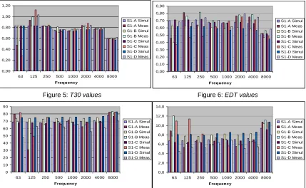
The values of T30, EDT, D50, C80, and Lp were measured in octave band intervals for the range

63- 8000 Hz. A model of the VA2 room was built on the computer and predictions were made with the new combined method. The diffusivity coefficients were determined by taking into account the typical values reported in the literature.

Simulated and measured values are shown in the n

5: T30 values Figure 6: EDT values

Figure 7: D50 values

ext figures.

Figure

0,00 0,20 0,40 0,60 0,80 1,00 1,20

63 125 250 500 1000 2000 4000 8000

Frequency

S1-A Simul S1-A Meas S1-B Simul S1-B Meas S1-C Simul S1-C Meas S1-D Simul S1-D Meas

0,00 0,10 0,20 0,30 0,40 0,50 0,60 0,70 0,80 0,90

63 125 250 500 1000 2000 4000 8000

Frequency

0 10 20 30 40 50 60 70 80 90

63 125 250 500 1000 2000 4000 8000

Frequency

0,0 2,0 4,0 6,0 8,0 10,0

63 125 250 500 1000 2000 4000 8000

Frequency

12,0 14,0

[image:7.595.87.516.441.705.2]

(8)

0,0 10,0 20,0 30,0 40,0 50,0 60,0 70,0 80,0

63 125 250 500 1000 2000 4000 8000

Frequency

[image:8.595.189.410.72.204.2]

Figure 9: Lp values

REFERENCES

[1] D. Alarcão, “Acoustic Modelling for Virtual Spaces”, PhD Thesis, IST, 2005.

[2] D. Alarcão and J.L. Bento Coelho, “A new combined method for the prediction of the room energy impulse response”, Paper 809 - Proceedings of ICSV12, Lisbon, Portugal. (2005)

[3] P. Hanrahan, D. Salzman and L. Aupperle; “A Rapid Hierarchical Radiosity Algorithm”, Computer

Graphics, 25(4):197-206, 1991.