Linguistic majorities with difference in support

Linguistic majorities with difference in support

Patrizia P´erez-Asurmendia_{, Francisco Chiclana}b,c,∗

a_{PRESAD Research Group, SEED Research Group, University of Valladolid, Valladolid, Spain} b_{Centre for Computational Intelligence, Faculty of Technology, De Montfort University, Leicester, UK}

c_{DMU Interdisciplinary Group in Intelligent Transport Systems, Faculty of Technology, De Montfort}

University, Leicester, UK

Abstract

Majorities based on difference of votes and their extension, majorities based on difference in support, were introduced in social choice voting as tools to implement the crisp prefe-rence values (votes) and the intensities of prefeprefe-rence provided by voters when comparing pairs of alternatives, respectively, with the aim to declare which alternative is socially preferred. Moreover, these rules require the winner alternative to reach a certain positive difference in its social valuation with respect to the one reached by the loser alternative. This paper introduces a new aggregation rule that extends majorities based on difference of votes from the context of crisp preferences to the framework of linguistic preferences. Under linguistic majorities with difference in support, the voters express their intensi-ties of preferences between pairs of alternatives using linguistic labels and an alternative defeats another one if the first one reaches a specific support fixed before the election process. There exist two main representation methodologies of linguistic preferences: the cardinal one based on the use of fuzzy set, and the ordinal one based on the use of the 2-tuples. Linguistic majorities with difference in support are formalised in both repre-sentation settings, and conditions are given to guarantee that fuzzy linguistic majorities and 2-tuple linguistic majorities are mathematically isomorphic. Moreover, linguistic majorities with difference in support constitute a class of majority rules because all the possible majority rules can be generalised to the linguistic framework by adjusting the required threshold of support. Finally, linguistic majorities based on difference in support are proved to verify relevant normative properties: anonymity, neutrality, monotonicity, weak Pareto and cancellativeness.

Keywords: Social choice, Aggregation rule, Linguistic preferences, Linguistic majorities, Fuzzy sets, 2-tuples, Difference in support.

1. Introduction

Decision making problems deal with the social choice of the best alternative among all the possible alternatives taking into account the views and opinions, i.e. the preferences, of all the individuals of a particular social group [8, 28, 32]. Two approaches are possible to address these problems [15, 17]: a direct approach that derives a social choice from the sole manipulation and processing of the information provided by all the individuals without the intermediate derivation of any kind of collective information using a fusion

∗_{Corresponding author}

Email addresses: [email protected](Patrizia P´erez-Asurmendi),[email protected]

or aggregation operator, which is characteristic of the indirect approach. Obviously, the type of aggregation rule implemented in the second approach is crucial in designing the corresponding social choice rule, and ultimately in the final social solution to the decision making problem. This paper deals with this specific issue, and it is devoted to the introduction of a new aggregation rule for individual preferences.

A comparison study between different alternative preference elicitation methods is reported in [26], where it was concluded that pairwise comparison methods are more ac-curate than non-pairwise methods. The main advantage of pairwise comparison methods is that facilitates individuals expressing their preferences because they focus exclusively on two alternatives at a time. Given two alternatives, an individual either prefers one to the other or is indifferent between them, which can be represented using a preference rela-tion whose elements represent the preference of one alternative over another one. There exist two main mathematical models to represent pairwise comparison of alternatives based on the concept of preference relation [8, 29]: in the first one, a preference relation is defined for each one of the above three possible preference states, which is usually referred to as a preference structure on the set of alternatives; the second one integrates the three possible preference states into a single preference relation. This paper deals with the second type of relations, for which reciprocity of preferences is usually assumed in order to guarantee the following basic rationality properties in making paired compar-isons [31]: indifference between any alternative and itself, and asymmetry of preferences, i.e. if an individual prefers alternative x to y, that individual does not simultaneously prefer y to x.

In classical voting systems the set of numerical values {1,0.5,0}, or its equivalent

{1,0,−1} [8], is used to represent when the first alternative is preferred to the second alternative, when both alternatives are considered equally preferred (indifference), and when the second alternative is preferred to the first one, respectively. This classical pre-ference modelling constitutes the simplest numeric discrimination model of prepre-ferences, and it proves insufficient in many decision making situations as the following example illustrates: Let {x, y, z}be 3 alternatives of which we know that one individual prefers x

to y and y toz, and another individual prefersz to y and y to x; then using the above numerical values it may be difficult or impossible to decide which alternative is the best. As Fishburn points out in [8], if alternative y is closer to the best alternative than to the worst one for both individuals then it might seem appropriate to ‘elect’ it as the social choice, whilst if it is closer to the worst than to the best, then it might be excluded from the choice set. Thus, in many cases it might be necessary the implementation of some kind of ‘intensity of preference’ between alternatives.

The concept of fuzzy set, which extends the classical concept of set, when applied to a classical relation leads to the concept of a fuzzy relation, which in turn allows the implementation of intensity of preferences [36]. In [2], we can find for the first time the fuzzy interpretation of intensity of preferences via the concept of a reciprocal fuzzy preference relation, which was later reinterpreted by Nurmi in [27]. In this approach, the numeric scale to evaluate intensity of preferences is the whole unit interval [0, 1] instead of {1,0.5,0}, which it is argued though to assume unlimited computational abilities and resources from the individuals [4].

hu-mans exhibit a remarkable capability to manipulate perceptions and other characteristics of physical and mental objects, without any exact numerical measurements and complex computations [3, 9, 16, 24, 38]. Therefore, in this paper, the individuals’ preferences between pair of alternatives will be assumed to be given in the form of linguistic labels.

It was mentioned before that the type of aggregation rule implemented is crucial in designing the corresponding social choice rule. This paper focuses on the majority voting rules, which are very easy to understand by voters and therefore, when comparing two alternatives, they are seen as very attractive and appropriate to aggregate individual preferences into a collective one. Simple majority rule [25] stands out among the different majority rules. Under this rule, an alternative defeats another one when the number of votes cast for the first one exceeds the number of votes cast for the second one. Simple majority rule states as the most decisive aggregation rule. In fact, the requirement to declare indifference between two alternatives is quite strong given that both alternatives have to receive exactly the same number of favourable votes. Furthermore, under the simple majority rule, the support required for an alternative to be the winner is minimum because it is only required to exceed the defeated alternative in just one vote. This characteristic turns out to become a drawback because the collective decision is very unstable, i.e. it could be reverted with the change of just one vote. In an attempt to overcome this shortcoming, tougher requirements for declaring an alternative as the winner have been defined and studied. Among these rules, it is worth mentioning the following: unanimous majority, absolute majority and qualified majority [7, 8, 30].

Majority based on difference of votes (Mk) [14, 19, 22] constitute a general approach

to majority voting rule that generalises all the above majority rules. This rule allows to calibrate the amount of support required for the winner alternative by means of a diffe-rence of votes fixed before the election process. At the extreme cases, i.e. no diffediffe-rence and maximum difference of votes, the majority based on difference of votes becomes the simple majority and unanimous majority, respectively. With this rule, indifference be-tween two alternatives is possible to be declared for more cases than under the simple majority rule. In fact, the indifference state could be enlarged as much as desired. The application of the majority based on difference of votes to the case of [0,1]-valued recip-rocal fuzzy preference relations is known as the majority based on difference in support

(Mf_k) [20].

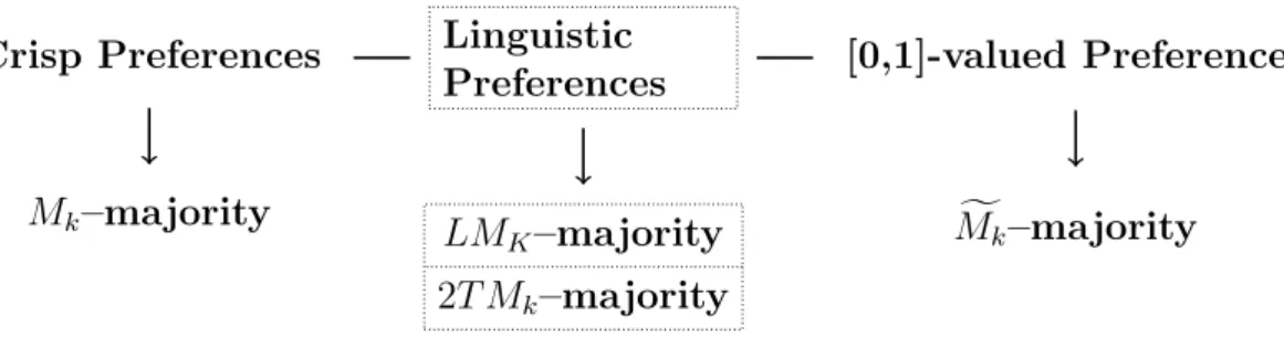
The aim of this paper is to fill the gap between the majority based on difference of votes and the majority based on difference in support by providing a new majority rule based on difference of support in the linguistic framework. Linguistic majority with difference in support keeps the essence of the former rules in the sense that for an alternative to be declared winner a specific support fixed before the election is to be achieved. The challenge here is to generalise formally the rule to the case of being the preferences linguistic rather than numeric in nature. An additional challenge here is to relate the linguistic majority with difference in support rules that can be obtained when the main two approaches to model and represent linguistic information are applied. On the one hand, linguistic preferences can be modelled using a cardinal approach by means of fuzzy sets and their associated membership functions [36]. On the other hand, an ordinal approach can be used to model and manage linguistic preferences using the 2–tuple symbolic representation [12]. Therefore, two new and different linguistic majority with difference in support rules will be introduced: the linguistic fuzzy majority (LMK) and

the 2–tuple linguistic majority (2T Mk). Figure 1 illustrates the new linguistic majorities

Linguistic Preferences

Crisp Preferences [0,1]-valued Preferences

Mk–majority _LM

K–majority

2T Mk–majority

f

Mk–majority

Figure 1: Preferences and Majorities based on differences

The remainder of the paper is structured as follows: The next section introduces con-cepts essential to the understanding of the rest of the paper. Following that, Section 3 introduces the concept of linguistic majority with difference in support and its mathema-tical formulation for the main two approaches to model and represent linguistic informa-tion: fuzzy set representation (Subsection 3.1) and the 2–tuple symbolic representation (Subsection 3.2). Section 4 proves that both linguistic majority rules are mathematically isomorphic when fuzzy sets are defuzzified into their centroid. In Section 5, the linguistic majority based on difference in support is proved to verify the following relevant norma-tive properties: anonymity, neutrality, monotonicity, weak Pareto and cancellanorma-tiveness. Lastly, Section 6 concludes the paper.

2. Preliminaries

Consider m voters provide their preferences on pairs of alternatives of a set X =

{x1, . . . , xn}. The preferences of each voter can be represented using a matrix, Rp =

r_ijp, where rp_ij stands for the degree or intensity of preference of alternative xi over

xj for voter p. The elements of Rp can be numerical values or linguistic labels. In the

following we focus on the former ones, leaving for Subsection 2.3 the second ones.

2.1. Numeric Preferences

There are two main types of numeric preference relations: crisp preference relations and [0,1]-valued preference relations; with the second one being an extension of the first one, i.e. [0,1]-valued preference relations have crisp relations as a particular case.

1. A crisp preference relation is characterised for having elements r_ijp that belong to the discrete set of values {0,1₂,1}. In this context, when alternatives are pairwise compared, voters declare only their preference for one of the alternatives or their indifference between the two alternatives. Thus, if rp_ij = 1 then voter p prefers alternative xi to alternative xj, while if rpij =

1

2 the voter p is indifferent between both alternatives. Moreover, it is always assumed that when rp_ij = 1₂ it is also

rp_ji = 1₂; and when rp_ij = 1 then r_jip = 0. This reciprocity property of preferences guarantees that the preferences are represented by a weak order, i.e. the asymmetric property is verified and ‘inconsistent’ situations where a voter could prefer two alternatives at the same time are avoided. Formally, a binary preference relation represented by p is asymmetric if given two alternatives xi and xj, xi p xj

2. The [0,1]-valued preference relation extends the crisp preference relation in that its elements rp_ij can take any value from the unit interval [0,1], with the following inter-pretation: r_ijp >0.5 indicates that the individual pprefers the alternative xi to the

alternative xj, with rpij = 1 being the maximum degree of preference forxi overxj;

rp_ij = 0.5 represents indifference between xi and xj for voter p. As in the previous

case, the reciprocity property of preferences, rp_ij+rp_ji = 1, is usually assumed as an extension of the crisp asymmetry property described above. This type of preference relations will be referred to as reciprocal preference relations in this paper. We note that, in probabilistic choice theory, reciprocal preference relations are referred to as probabilistic binary preference relations. In fuzzy set theory, reciprocal preference relations when used to represent intensities of preferences have usually been referred to as reciprocal fuzzy preference relations. Reciprocal preference relations can be seen as a particular case of (weakly) complete fuzzy preference relations, i.e. fuzzy preference relations satisfying rij +rji ≥1 ∀i, j.

2.2. Majority based on differences

In an attempt to overcome the support problems commonly attached to the simple majority rule in decision-making contexts with crisp preferences, Garc´ıa-Lapresta and Llamazares [19] formalise the concept of majority based on difference of votes or Mk–

majority, which was later axiomatically characterised in [14, 22].

Definition 1 (Mk–majority). Given k ∈ {0, . . . , m−1}, and a profile of individual

crisp preferences R(X) = (R1_{, . . . , R}m_{) on a set of alternatives X = {x}

1, . . . , xn}, the

Mk–majority is a collective profile of crisp preferences on X, i.e. a mapping from X×X

to {1,1₂,0}, with the following expression:

Mk(xi, xj) = 

   

   

1 if mi > mj +k

0 if mj > mi+k

1

2 otherwise,

where mi is the number of votes cast by the individuals for the alternative xi and mj is

the number of votes cast for the alternative xj.

Thus, under theMk–majority, given a difference of votes k, an alternative, xi, defeats

another alternative, xj, by k votes (Mk(xi, xj) = 1) when the difference between the

votes cast for the alternative xi and the votes cast for the alternative xj is greater than

k. Compared with the simple majority rule, the main change introduced by the majority based on difference of votes affect the indifference state. The indifference of preference between two alternatives happens when the difference between the votes cast for both alternatives in absolute value is lower than or equal to k, i.e. when the difference of votes belongs to{0,1, . . . , k}.

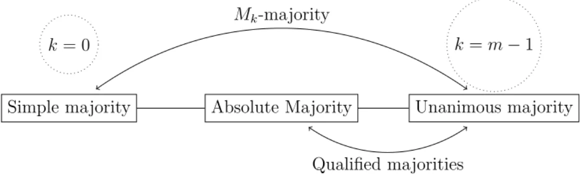
Mk–majority generalises other majority rules. In particular, M0–majority is the simple majority rule, whereas M(m−1)–majority is the unanimous majority rule. More-over, Mk–majority and qualified majorities, which are located between absolute majority

and unanimity, are equivalent when individual indifference is ruled out from individual preferences. These facts are summarized in Figure 2.

Garc´ıa-Lapresta and Llamazares extend Mk–majority to the framework of [0,1]–

Absolute Majority Simple majority

k = 0

Unanimous majority

k=m−1

Mk-majority

Qualified majorities

Figure 2: Mk–majorityversus other majorities.

voters to show their preferences between pairs of alternatives through reciprocal prefe-rence relations whilst still maintaining the requirement of a higher support to the winner alternative than with the simple majority rule. Under Mfk–majority, an alternative, xi,

defeats another one, xj, by a threshold of support k, when the sum of the intensities of

preference of xi over xj for the m voters exceeds the sum of the intensities of preference

of xj over xi in a quantity greater than k.

Definition 2 (Mf_k–majority). Given a threshold k ∈[0, m) and a profile of individual

reciprocal preference relations R(X) = (R1_{, . . . , R}m_{), the} f

Mk–majority is a collective

profile of crisp preferences on X, i.e. a mapping from X × X to {1,1₂,0}, with the following expression:

f

Mk(xi, xj) = 

    

    

1 if

m P

p=1

r_ijp >

m P

p=1

r_jip +k

0 if

m P

p=1

r_jip >

m P

p=1

r_ijp +k

1

2 otherwise,

Note that with Mf_k–majority, indifference between two alternative happens when the

difference in support between the alternatives in absolute value is lower than or equal to

k, i.e. it is a value in the closed interval [0, k].

A direct consequence of the reciprocity property is that Mfk–majority can be

equiva-lently expressed in terms of the average of individual intensities of preference [20]:

f

Mk(xi, xj) = 

    

    

1 if _m1

m P

p=1

r_ijp > m₂+_mk

0 if _m1

m P

p=1

r_ijp < m−k_2m

1

2 otherwise.

(1)

The term _m1

m P

p=1

rp_ij can be interpreted as the collective preference (the average of all the votes) of the first alternative, xi, over the second one, xj. Under the Mfk–majority rule,

to the closed interval

0.5− k

2m,0.5 + k

2m

, which we refer to as the indifference interval. When the collective preference is greater than the upper bound of the indifference interval, the first alternative is preferred to the second one. On the other hand, when the collective preference is lower than the lower bound of the indifference interval, the second alternative is preferred to the first one. In comparison with the simple majority rule, theMf_k–majority

rule promotes an increase on the cases where the collective indifference is declared, which depends on the threshold of support required to define the strict preference state.

2.3. Linguistic Preferences

As mentioned before, subjectivity, imprecision and vagueness in the articulation of opinions pervade real world decision applications, and individuals might feel more com-fortable using words by means of linguistic labels or terms to articulate their preferences [37]. In these cases is still valid the following quotation by Zadeh [38]: “Since words, in general, are less precise than numbers, the concept of a linguistic variable serves the purpose of providing a means of approximate characterization of phenomena which are too complex or too ill-defined to be amenable to description in conventional quantitative terms.”

Let L = {l0, . . . , ls}be a set of linguistic labels (s ≥ 2), with semantic underlying a

ranking relation that can be precisely captured with a linear order, i.e., l0 < l1 < . . . <

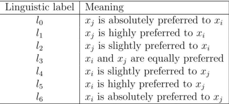
ls. In Table 1, an example with seven linguistic labels and their corresponding semantic

meanings for the comparison of the ordered pair of alternatives (xi, xj).

Linguistic label Meaning

l0 xj is absolutely preferred to xi

l1 xj is highly preferred to xi

l2 xj is slightly preferred to xi

l3 xi and xj are equally preferred

l4 xi is slightly preferred to xj

l5 xi is highly preferred to xj

l6 xi is absolutely preferred to xj

Table 1: Seven linguistic labels

Assuming that the number of labels is odd and the central labells/2 stands for the in-difference state when comparing two alternatives, the remaining labels are usually located symmetrically around that central assessment, which guarantees that a kid of reciprocity property holds as in the case of numerical preferences previously discussed. Thus, if the linguistic assessment associated to the pair of alternatives (xi, xj) islij =lh ∈ L, then the

linguistic assessment corresponding to the pair of alternatives (xj, xi) would belji =ls−h.

Therefore, the operator defined as N(lh) = lg with (g +h) = s is a negator operator

because N(N(lh)) =N(lg) = lh.

The corresponding matrix notation of linguistic individual preferences of voter p is

R = (lp_ij) with lp_ij ∈ L. A profile of linguistic preferences for the pair of alternatives (xi, xj) is the vector of its associated linguistic preferences given by a set of m voters,

(l1_ij, . . . , l_ijm) ∈ Lm_{. The main two representation formats of linguistic information are}

2.3.1. Fuzzy set linguistic representation format

Convex normal fuzzy subsets of the real line, also known as fuzzy numbers, are com-monly used to represent linguistic terms. By doing this, each linguistic assessment is represented using a fuzzy number that is characterized by a membership function, with base variable the unit interval [0,1], describing its semantic meaning. The membership function maps each value in [0,1] to a degree of performance which represents its com-patibility with the linguistic assessment [37]. Figure 3 illustrates a fuzzy number with Gaussian membership function.

0 0.43 0.5 0.57 1

0 0.2 0.4 0.6 0.8 1

µτ

Figure 3: Representation of a fuzzy number with Gaussian membership function

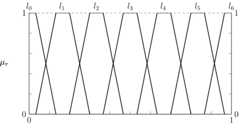
It is worth mentioning that some authors consider trapezoidal fuzzy numbers as the most appropriate to represent linguistic preferences [5, 21] because they are more general than triangular and interval fuzzy numbers. Given four real numbers t1, t2, t3, t4, a trapezoidal fuzzy number (TFN) τ = (t1, t2, t3, t4) is characterised by the the following membership function:

µτ(u) = 

    

    

0, if u < t1 or u > t4

u−t1

t2−t1, if t1 < u < t2

1, if t2 ≤u≤t3

t4−u

t4−t3, if t3 < u < t4.

(2)

0 1 0

1l0 l1 l2 l3 l4 l5 l6

µτ

0 1

µτ

Figure 4: Representation of seven balanced linguistic terms with trapezoidal membership functions

2.3.2. 2–tuple linguistic representation format

Linguistic assessments can also be represented and aggregated using symbolic repre-sentation models based on an ordinal interpretation of the semantic meaning associated to the linguistic labels. Within this framework, the following different approaches have being developed: a linguistic symbolic computational model based on ordinal scales and max-min operators [34], a linguistic symbolic computational model based on indexes [6, 33].

In Herrera and Martinez [12], a more general approach was introduced: the 2-tuple linguistic model. This linguistic model takes as a basis the symbolic representation model based on indexes and in addition defines the concept of symbolic translation to represent the linguistic information by means of a pair of values called linguistic 2-tuple, (lb, λb),

wherelb ∈ Lis one of the original linguistic terms andλb is a numeric value representing

the symbolic translation. This representation structure allows, on the one hand, to obtain the same information than with the symbolic representation model based on indexes without losing information in the aggregation phase. On the other hand, the result of the aggregation is expressed on the same domain as the one of the initial linguistic labels and therefore, the well-known re-translation problem of the above methods is avoided.

Definition 3 (Linguistic 2–tuple representation). Let a ∈ [0, s] be the result of a symbolic aggregation of the indexes of a set of labels assessed in a linguistic term set

L = {l0, . . . , ls}. Let b = round(a) ∈ {0, . . . , s}. The value λb = a−b ∈ [−0.5,0.5) is

called a symbolic translation, and the pair of values (lb, λb) is called the 2–tuple linguistic

representation of the symbolic aggregationa.

The 2–tuple linguistic representation of symbolic aggregation can be mathematically formalised with the following mapping:

φ : [0, s] → L × [−0.5,0.5)

φ(a) = (lb, λb).

(3)

Based on the linear order of the linguistic term set and the complete ordering of the set [−0.5, 0.5), it is easy to prove that φ is strictly increasing and continuous and, therefore its inverse function exists:

φ−1 : L × [−0.5,0.5) → [0, s]

φ−1_(l

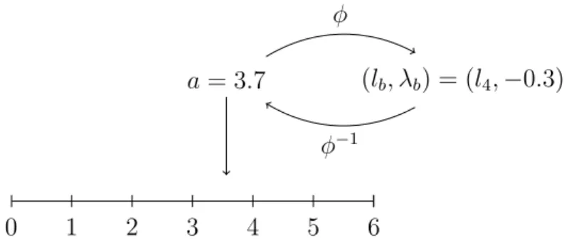
The following negation operator is defined: N(φ(a)) =φ(s−a). Figure 5 illustrates the application of the 2-tuple functionφand its inverse for a linguistic term set of cardinality seven. The value of the symbolic translation is assumed to be 3.7, which means that

round(3.7) = 4 and therefore it can be represented with the 2-tuple (l4,−0,3).

a= 3.7 (lb, λb) = (l4,−0.3)

φ

φ−1

0 1 2 3 4 5 6

Figure 5: Ordinal linguistic representation: symbolic translation and 2-tuples

3. Linguistic majorities with difference in support

Before majority rules based on difference of votes in the context of linguistic prefer-ences are defined, we need to introduce the linguistic decision rule concept. Recall that a profile of linguistic preferences for a pair of alternatives alternatives (xi, xj) is a vector

of its associated linguistic preferences given by a set of m voters (l1

ij, . . . , lijm) ∈ Lm. Definition 4. Given a pair of alternatives (xi, xj)∈X×X a linguistic decision rule is

a mapping

F : Lm _{→ {0,0.5,1},}

such that:

F(l1_ij, . . . , lm_ij) =







1 if xi defeats xj;

0 if xj defeats xi,;

0.5 if xi and xj tie.

The generalisation of the majority based on difference of votes from the context of numerical preferences to the linguistic one involves: (1) the computation of the voters average linguistic assessment for a pair of alternatives, and (2) the evaluation of the difference between two linguistic evaluations. In the following, we will formalise this in both linguistic representation methodologies.

3.1. Fuzzy linguistic majority with difference in support

In what follows, Aep_ij denotes the normal and convex fuzzy set representing the

lin-guistic preference of alternative xi over xj provided by voter p. As mentioned before,

the formalisation of the fuzzy linguistic majority with difference in support requires the computation of the average fuzzy linguistic preference, 1

m m P

p=1

e

Ap_ij, of a profile of linguistic

preferences Ae1_ij, . . . ,Aem_ij

.

Definition 5 (Extension Principle). Let X1×X2×. . .×Xn be a universal product

set and F a functional mapping of the form

F: X1×X2×. . .×Xn −→Y

that maps the element (x1, x2, . . . , xn) ∈ X1 × X2 × . . . × Xn to the element y =

F(x1, x2, . . . , xn) of the universal set Y. Let Ae_i be a fuzzy set over the universal set

Xi with membership function {µAei(xi)|xi ∈ Xi} (i = 1,2, . . . , n). The membership

function {µ_Be(y)|y∈Y} of the fuzzy set Be over the universal setY

e

B =F(Ae₁,Ae₂, . . . ,Ae_n)

is

µ_Be(y) =







sup

y=F(x1,x2,...,xn)

µ

e

A1(x1)∗µAe2(x2)∗. . .∗µAen(xn)

if ∃y =F(x1, x2, . . . , xn)

0 otherwise.

(4) where ∗ is a t-norm.

For the work presented in this paper, the minimum t-norm (∧) is used.

In what follows we will first extend the real function f: [0,1]×[0,1]−→[0,1], f(u1, u2) =u1+u2,

to f(Ae1,Ae2) where Ae1,Ae2 are over the set [0,1] and associated membership functions

µ_Ae

1(u1), µAe2(u2), with u1, u2 ∈[0,1]. The extension principle states that Be =f(Ae1,Ae2)

is a fuzzy set over the set [0,1] with membership function µ_Be: [0,1]→[0,1];

µ

e

B(u) = sup u1+u2=u u1,u2∈[0,1]

µ

e

A1(u1)∧µAe2(u2)

.

The representation theorem of fuzzy sets [36] provides an alternative and convenient way to define a fuzzy set via its corresponding family of crisp α-level sets. The α-level set of a fuzzy set Aeover the universe Z is defined as Aeα ={z ∈Z|µ

e

A(z)≥ α}. The set

of crisp sets {Aeα|0 < α ≤ 1} is said to be a representation of the fuzzy set A. Indeed,

the fuzzy set Aecan be represented as

e

A= ∪

0<α≤1αAe

α

with membership function

µ_Ae(z) = sup

α:z∈Aeα

α.

Let Aeα₁ and Aeα₂ be the α-level sets of fuzzy sets Ae₁ and Ae₂ described above. We have

fAeα₁ ×Aeα₂

=nu1 +u2|u1 ∈Aeα₁, u₂ ∈Aeα₂ o

.

Both Beα and f

e

Aα

1 ×Aeα₂

I. Letu∈Beα. By definition, we haveµ

e

B(u)≥αand there exists at least three values

u1, u2 ∈[0,1] such that u1 +x2 = u and

µ

e

A1(u1)∧µAe2(u2)

≥ α. Therefore, it is true that µ

e

A1(u1) ≥α and µAe2(u2)≥ α, which means that u1 ∈ Ae α

1 and u2 ∈ Aeα₂.

Consequently, u∈f

e

Aα₁ ×Aeα₂

, i.e. Beα ⊆f(Aα₁ ×Aα₂).

II. Let u ∈ fAeα₁ ×Aeα₂

. There exist u1 ∈ Aeα₁ and u₂ ∈ Aeα₂ such that u₁ +u₂ = u.

We have that µ

e

A1(u1)≥α and µAe2(u2)≥α and therefore it is:

sup

u1+u2=u u1∈Aeα₁,u2∈Aeα₂

µ_Ae

1(u1)∧µAe2(u2)

≥α.

Because Aeα₁,Aeα₂ ⊆[0,1] then we have:

sup

u1+u2=u u1,u2∈[0,1]

µ_Ae

1(u1)∧µAe2(u2)

≥ sup

u1+u2=u u1∈Aeα₁,u2∈Aeα₂

µ_Ae

1(u1)∧µAe2(u2)

.

We conclude thatu∈Beα, i.e. f

e

Aα

1 ×Aeα₂

⊆Beα.

Therefore, we have the following equality:

Bα =f(Aα₁ ×Aα₂). (5) A similar reasoning will lead us to conclude that the α–level set of the average of fuzzy numbers is equal to the average of the α–level set of fuzzy sets [39]. Denoting

f(Aα₁ ×Aα₂) = Aeα₁ +Aeα₂, it is safe to use the following notation

e

B =Ae₁+Ae₂ ⇐⇒

e

A1+Ae₂ α

=Aeα₁ +Aeα₂.

The α–level sets of fuzzy numbers are closed intervals, and therefore interval arithmetic yields:

e

A1+Ae2

α

=Aeα₁ +Ae₂α = [u−₁, u+₁] + [u₂−, u+₂] = [u−₁ +u−₂, u+₁ +u+₂].

An example of the addition using theα–level sets is shown in Figure 6. Given the fuzzy numbers l3 and l4 (Figure 4), l3+l4 is constructed by applying (5) to compute the lower and upper bounds of its α–level sets, followed by the application of the representation theorem of fuzzy sets. The computation of the lower bound of the 0.2–level set is given.

0 0.386 0.553 0.939 2

0 0.2

1 l3 l4 l3+l4

Real numbers

α–level

Once we have solved the computation of the average linguistic preference of the profile of linguistic preferences associated to a pair of alternatives, the formalisation of the fuzzy linguistic majority with difference in support requires its classification regarding its containment in one of the intervals corresponding to the social preference or social indifference established by the Mf_k–majority. In other words, we need to find out when

the following inequality _m1

m P

p=1

e

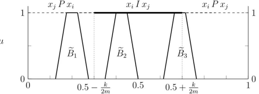
Ap_ij > m₂+_mk is true or when it is false. Because crisp numbers are particular types of fuzzy numbers, the above inequality involves the comparison of fuzzy numbers. Yager [35], pointed out that this problem has been extensively studied and that there is no unique best approach. Indeed, the set of fuzzy numbers is not totally ordered and therefore it is not possible to achieve a clear social decision in this case. This is clearly illustrated in Figure 7, where three different aggregated fuzzy set are displayed, namely Be₁, Be₂ and Be₃. Note that because Be₁ and Be₂ completely belong

to the interval of preference for xj and to the interval of indifference between both

alternatives, respectively, there is no doubt about the social decision in these cases. On the contrary, the case represented by Be₃ is ambiguous given that such set is located in

between the interval of preference for xi and the indifference state. Thus, a different

approach is needed if we are to provide a clear cut social choice as per Definition 4.

0 _0.5− k

2m 0.5 0.5 + k

2m 1

0 1

e

B1 Be₂ Be₃

xiI xj

xjP xi xiP xj

µ

0 1

Figure 7: Comparison between aggregated fuzzy sets and preference or indifference states.

A widely used approach to rank fuzzy numbers consist in converting them into a representative crisp value, and perform the comparison on them [35]. Two defuzzification methods widely used are: the centre of area method (COA) and the mean of maximum method (MOM). The first one computes the centre of mass of the membership function of the fuzzy set (the centroid), whereas the second one computes the mid-point of the 1–level set of the fuzzy set.

For a trapezoidal fuzzy number Aewith membership function (2), we haveu_COA(Ae) = t1+t4

2 and uM OM(Ae) =

t2+t3

2 . Under the assumed property of internal symmetry of the linguistic labels, it is clear that both values coincide. Therefore, we refer to these real numbers simply as u(Ae). Also, given two trapezoidal fuzzy numbers, namelyAe₁ and Ae₂,

it holds that u(Ae1+Ae2) =u(Ae1) +u(Ae2). Hence, u is an additive function.

Note that the range of function u is [u(l0), u(ls)], while the range of m₂+_mk is [0,1].

Thus, to carry out a fair comparison in the formalisation of the linguistic majority with difference in support, the following function u’ with range [0, 1] is used:

u’(Ae) =

u(Ae) − u(l₀) u(ls) − u(l0)

Below, we formally define the linguistic majority with difference in support represented by fuzzy sets. Under this rule, an alternative, say xi, defeats another one, say xj by a

threshold of support K, if the defuzzified value attached to the average fuzzy set of the voters’ linguistic valuations between xi and xj exceeds the value 0.5 in a quantity that

depends on the threshold K, fixed before the election process.

Definition 6 (LMK–majority with difference in support). Given a set of

alterna-tivesX and a profile of individual reciprocal fuzzy linguistic preference relations R(X) = (R1, . . . , Rm), theLMK–majority with difference in support is the following linguistic

de-cision rule:

LMK(Ae1_ij, . . . , Aem_ij) =             

1 if u’ 1 m m P p=1 e

Ap_ij

> m+K

2m

0 if u’ 1 m m P p=1 e

Ap_ij

< m−K_2m

0.5 otherwise.

(6) where u’ 1 m m P p=1 e

Ap_ij

is the defuzzified value of the fuzzy average linguistic preference of the profile of fuzzy linguistic preferences of the pair of alternatives (xi, xj); and K ∈

[0, m) represents the threshold of support required for an alternative to be the social winner.

In the following result we prove that function u’ is additive:

Proposition 1. Function u’ verifies

u’ 1 m m X p=1 e

Ap_ij

! = 1 m m X p=1

u’(Aep_ij).

Proof. Because u is additive we have that

u 1 m m X p=1 e

Ap_ij

! = 1 m m X p=1

u(Ae p ij).

Also, we have that u and u’ are related in the form u ≡ c · u’ + d where c =

u(lh) − u(l0) and d = u(l0), it is:

u 1 m m X p=1 e

Ap_ij

!

= c · u’ 1

m

m X

p=1

e

Ap_ij

! +d u 1 m m X p=1 e

Ap_ij

! = 1 m m X p=1

u(Ae p ij) =

1 m m X p=1 h

c · u’(Ae p ij) + d

i !

= c · 1

m

m X

p=1

u’(Aep_ij) +d.

Thus, we have:

u’ 1 m m X p=1 e

Ap_ij

! = 1 m m X p=1

u’(Ae p ij),

Therefore expression (6) can be rewritten as follows:

LMK(Ae1_ij, . . . , Aem_ij) = 

     

     

1 if _m1

m P

p=1

u’(Ae p ij)>

m+K

2m

0 if _m1

m P

p=1

u’(Aep_ij)< m−K_2m

0.5 otherwise,

(7)

with K ∈ [0, m) and _m1

m P

p=1

u’(Aep_ij) is the average of the defuzzified values associated

with the profile of fuzzy linguistic preferences of the pair of alternatives (xi, xj) as per

the assessment of each individual voter.

In the following, we provide an example to illustrate the application of the LMK–

majority with difference in support.

Example 1. Consider nine voters expressing their preferences between two alternatives, (xi, xj), using the linguistic labels of Table 1. We use the set of trapezoidal fuzzy numbers

of Table 2, which were represented in Figure 4, to represent the linguistic information:

Linguistic label Trapezoidal fuzzy number u(lh) u’(lh)

l0 (0, 0, 0.033, 0.133) 0.016 0

l1 (0.033, 0.133, 0.2, 0.3) 0.166 0.155

l2 (0.2, 0.3, 0.366, 0.466) 0.333 0.327

l3 (0.366, 0.466, 0.533, 0.633) 0.5 0.5

l4 (0.533, 0.633, 0.7, 0.8) 0.666 0.672

l5 (0.7, 0.8, 0.866, 0.966) 0.833 0.844

l6 (0.866, 0.966, 1, 1) 0.983 1

Table 2: Trapezoidal fuzzy numbers and centroids.

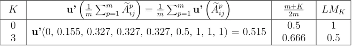
For the following profile of linguistic preferences (l0, l1, l2, l2, l2, l3, l6, l6, l6), we compute in Table 3 two differentLMK–majorities with difference in support: the simple linguistic

majority LM0, and LM3. In the first case, it is enough to have an average centroid of the linguistic profile greater than the centroid (0.5) of the central linguistic assessment (l3). In the second case, the threshold required implies that the average centroid of the linguistic profile is to be greater than the centroid of the linguistic label l4. In the first case, we have that xi is the social winner, whilst there is social indifference in the second

case.

K u’_m1 Pm_p=1Aep_ij

= _m1 Pm_p=1u’Aep_ij

m+K

2m LMK

0

3 u’(0, 0.155, 0.327, 0.327, 0.327, 0.5, 1, 1, 1) = 0.515

0.5 0.666

1 0.5 Table 3: Aggregation and results for two different LMK–majorities

• TheLMK–majority with difference in support generalises thesimple linguistic

ma-jority [18]. Indeed, LM0–majority coincides with the simple majority based on linguistic labels. In this case, no difference of support between the alternatives is required.

• Linguistic unanimity holds when all the voters involved in the election prefer the same alternative, even when their intensities of preference could differ from one to another. The following three linguistic profiles with nine voters and a set of seven linguistic terms will serve to illustrate this concept.

(l0, l0, l0, l1, l1, l1, l2, l2, l2); (l6, l6, l6, l6, l6, l6, l6, l6, l6); (l0, l0, l0, l0, l0, l0, l0, l0, l3).

The first two profiles fulfil linguistic unanimity: in the first one all nine voters express a preference for the second alternative, whilst in the second one the first alternative is preferred by all nine voters. However, in the third profile there is no unanimity of preferences because voter 9 expresses indifference between both alternatives and therefore differs from the rest of voters, who strongly prefer the second alternative:

Given a profile of fuzzy linguistic preferences (Ae1_ij, . . . ,Aem_ij), linguistic unanimity

happens ifu’(Aep_ij)≤u’(ls

2−1) (∀p), oru’(Ae p

ij)≥u’(ls2+1) (∀p). In the first case, all

voters prefer the second alternative over the first one, whilst the first alternative is preferred over the second one in the second case. Algebraic manipulation leads us to the following threshold values: K > m−2m·u’(ls

2−1) for the social preference

of the second alternative, and K > 2m·u’(ls

2+1)−m for the social preference of

the first alternative.

Because we are assuming that the linguistic labels are symmetrical and balanced around the central one, then if the fuzzy sets used to represent them are all of the same type and uniformly distributed in the domain [0,1], the normalised centroid functionu’would beu’(lh) =h/s (∀h), and therefore the threshold value to assure

linguistic unanimity would be K >2m/s.

3.2. 2–tuple linguistic majority with difference in support

In order to extend the Mk–majority to the framework of the 2–tuple, the addition as

well as a rule to compare 2–tuples are needed.

Definition 7 (2–tuple Addition [12]). The addition of 2–tuples, φ(a1) = (lb1, λb1)

and φ(a2) = (lb2, λb2), with b1 = round(a1), b2 = round(a2), λb1 = a1 − b1 and

λb2 = a2 −b2, is computed as follows:

φ(a1) +φ(a2) = (lb12, λb12),

with b12 = round(a1+a2), and λb12 = (a1+a2)−b12.

Definition 8 (2–tuple Lexicographic Ordering [12]). Given φ(a1) = (lb1, λb1) and

φ(a2) = (lb2, λb2), we have that,

1. If b1 is greater than b2, then φ(a1)> φ(a2).

3. If b1 is equal to b2 and λb1 is equal to λb1, then φ(a1) =φ(a2).

Below, we formally define the 2–tuple linguistic majority with difference in support. Under this rule, an alternative, say xi, defeats another one, say xj by a threshold of

support k, if the 2–tuple linguistic representation of the average symbolic aggregation of the linguistic preferences of xi over xj exceeds the 2–tuple linguistic representation

associated to the indifference state in a value that depends on the threshold k, fixed before the election process.

Definition 9 (2T Mk–majority with difference in support). Given a set of

alter-natives X and a profile of individual reciprocal 2–tuple linguistic preference relations

R(X) = (R1, . . . , Rm), the 2T Mk–majority with difference in support is the following

linguistic decision rule:

2T Mk(a1ij, . . . , a p ij) =

            

1 if _m1

m P

p=1

φ ap_ij > φ s·m_2m+k

0 if _m1

m P

p=1

φ ap_ij < φ s·m_2m−k

0.5 otherwise.

(8)

where _m1

m P

p=1

φ ap_ijis the average of the 2–tuple representation of the linguistic preferences provided by the voters for the pair of alternatives (xi, xj), φ is the 2–tuple symbolic

aggregation mapping (3); and k ∈[0, m·s) represents the threshold of support required for an alternative to be the social winner.

We note that in the context of the 2–tuple linguistic representation, the linguistic label lh is associated a valuation that coincides with its ordering position within L, i.e.

h, and therefore the maximum social preference value a set of voters can assign to an alternative when compared against another one ism·s, which corresponds to the linguistic profile (ls,· · · , ls). This explains why [0, m·s) is the range of values for parameter k.

Given that in the ordinal representation of linguistic information the addition of lin-guistic labels is defined asla1 +la2 =la1+a2 [33], it is obvious that function φ is additive.

Therefore expression (8) can be rewritten as follows:

2T Mk(a1ij, . . . , a p ij) =

            

1 if φ

1 m m P p=1

ap_ij

> φ s·m_2m+k

0 if φ

1 m m P p=1

ap_ij

< φ s·m_2m−k

0.5 otherwise.

(9)

where _m1

m P

p=1

ap_ij is the symbolic aggregation, specifically the arithmetic mean, of the lin-guistic preferences provided by the voters for the pair of alternatives (xi, xj).

The following example illustrates the use of the 2T Mk–majority with difference in

support:

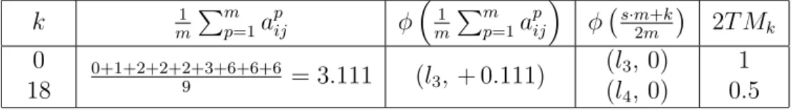
winner when the 2-tuple representation of the symbolic arithmetic mean of the linguistic preferences provided by the voters for the pair of alternatives (xi, xj) is greater than

the indifference 2-tuple (l3, 0); while it has to be greater than the 2–tuple (l4, 0) in the second case.

k _m1 Pm_p=1ap_ij φ_m1 Pm_p=1ap_ij φ s·m_2m+k

2T Mk

0 18

0+1+2+2+2+3+6+6+6

9 = 3.111 (l3, + 0.111)

(l3, 0) (l4, 0)

1 0.5 Table 4: Aggregation and results for two different 2T Mk–majorities

Examples 1 and 2 let us hypothesise that LMK–majority and 2T Mk–majority

coin-cide when the following relationship hold K =k/s. This will be proven in the following section.

4. Equivalence betweenLMK and 2T Mk majorities with difference in support

So far, we have provided two apparently different extensions of Mk–majorities to the

framework of the linguistic preferences. In this section, we prove that LMK and 2T Mk

are equivalent.

Let lh ∈ L be a linguistic label, u(lh) and φ(lh) its associated centroid and 2-tuple

representation. Let δ be the function that maps φ(lh) into u’(lh), i.e.

δ(φ(lh)) =u’(lh). (10)

Note that the following equivalence is true φ(la) ≡ a, and therefore it is true that the

above function δ is the restriction of a continuous and strictly increasing function with domain [0, s]:

δ: [0, s]−→[0,1] such that δ(0) = 0, δ(s/2) = 0 and δ(s) = 1.

Theorem 1 (LMK and 2T Mk Equivalence). If δ is additive then LMK–majority is

equivalent to 2T Mk–majority.

Proof. The following results is well known: if a continuous function verifies F(x+y) =

F(x) +F(y) ∀x, y ∈_Rthen there exists a constant a∈_Rsuch that F(x) = a·x ∀x∈_R

[1]. This result applied to function δ implies that δ(x) = x/s.Therefore we have:

1

m

m X

p=1

u’(Ae p ij) >

m+K

2m ⇔

1

m

m X

p=1

δ

φ(Ae p ij)

> m+K

2m ,

i.e.

1

m

m X

p=1

u’(Aep_ij) >

m+K

2m ⇔

1

m

m X

p=1

φ(Aep_ij) >

s·m+s·K

2m .

We conclude that LMK–majority is equivalent to 2T Mk–majority when k =s·K.

Theorem 1 establishes the condition for LMK–majority and 2T Mk–majority to be

mathematically isomorphic: δ(x) = x/s. In the following section we prove a number of normative properties for the 2T Mk–majority with difference in support, which obviously

5. Properties of linguistic majorities with difference in support

For convenience, we use Expression (8) for 2T Mk–majority with difference in support:

2T Mk(a1ij, . . . , a p ij) =



     

     

1 if _m1

m P

p=1

φ ap_ij > φ s·m_2m+k

0 if _m1

m P

p=1

φ ap_ij

< φ s·m_2m−k

0.5 otherwise.

where _m1

m P

p=1

φ ap_ijis the average of the 2–tuple representation of the linguistic preferences provided by the voters for the pair of alternatives (xi, xj), φ is the 2–tuple symbolic

aggregation mapping (3); and k ∈[0, m·s) represents the threshold of support required for an alternative to be the social winner.

The first normative property that 2T Mk–majority fulfils is anonymity, i.e. the order

in which the linguistic valuations of the voters are given is irrelevant for the final social outcome. Indeed, this is a direct consequence of the arithmetic mean being commutative.

Proposition 2 (Anonimity). Given a profile of linguistic preferences (l1, . . . , lm) ∈ Lm_,

the following equality holds

2T Mk(l1, . . . , lm) = 2T Mk(lσ(1), . . . , lσ(m)).

for any permutation σ : {1, . . . , m} → {1, . . . , m}.

Neutrality means that the aggregation rule should treat alternatives equally. In the proposition bellow, that property is proven.

Proposition 3 (Neutrality). Given a profile of linguistic preferences (l1_{, . . . , l}m_{) ∈ L}m_,

The following equality holds

2T Mk(N(l1), . . . , N(lm)) = 1− 2T Mk(l1, . . . , lm).

Proof. We have to prove the following three statements.

1. If 2T Mk(N(a1ij), . . . , N(amij)) = 1, then 2T Mk(a1ij, . . . , amij) = 0.

2. If 2T Mk(N(a1ij), . . . , N(amij)) = 0, then 2T Mk(a1ij, . . . , amij) = 1.

3. If 2T Mk(N(a1ij), . . . , N(amij)) = 0.5, then 2T Mk(a1ij, . . . , amij) = 0.5.

Given a profile of linguistic preferences, (l1_{, . . . , l}m_{), the first step is to express it in}

terms of its equivalent symbolic translation, i.e., (a1_{, . . . , a}m_{), and therefore we have that}

lp ≡φ(ap) and N(lp)≡N(φ(ap)) =φ(s−ap) =φ(s)−φ(ap) =s−φ(ap).

We have 1

m

m X

p=1

N(φ(ap)) = 1

m

m X

p=1

(s−φ(ap)) =s− 1

m

m X

p=1

φ(ap)

and

φ(s)−φ

s·m+k

2m

=φ

s·m−k

2m

Thus

1

m

m X

p=1

N(φ(ap))> φ

s·m+k

2m

⇔ 1

m

m X

p=1

φ(ap)< φ

s·m−k

2m

,

which proves item 1. The proof of items 2 and 3 are similar.

Monotonicity is proven next. Under this property, the majority value does not de-crease when the individual linguistic preference evaluation of a profile inde-crease.

Proposition 4 (Monotonicity). Given two profiles of linguistic preferences, (l1_{, . . . , l}m₎

and (l01, . . . , l0m), such that it holds that li ≥l0i (∀i) then:

2T Mk(l1, . . . , lm) ≥ 2T Mk(l 0₁

, . . . , l0m).

Proof. Recall that both functionφand the arithmetic mean are increasing, and therefore denoting li ≡φ(ap) and l0i ≡φ(a0p) we have

li ≥l0i ⇒ 1

m

m X

p=1

φ(ap)≥ 1

m

m X

p=1

φ(a0p),

which proves that

2T Mk(l1, . . . , lm) ≥ 2T Mk(l 0₁

, . . . , l0m).

The weak Pareto property presented below, asserts that the result under the rule has to respect unanimous profiles.

Proposition 5 (Weak Pareto). The following equalities hold: 1. 2T Mk(ls, . . . , ls) = 1

2. 2T Mk(l0, . . . , l0) = 0.

Proof. On the one hand, we have

1

m

m X

p=1

φ(s) = φ(s) ≥ φ

m·s+k

2m

(∀k),

and therefore

2T Mk(ls, . . . , ls) = 1.

On the other hand 1

m

m X

p=1

φ(0) =φ(0) ≤ φ

m·s−k

2m

(∀k),

and therefore

Finally, the cancellative property is proven. Given two profiles with same linguistic labels but two of them, then if the addition of the symbolic translations of the differing linguistic labels in each profile coincide, then the social majority is the same for the two profiles.

Proposition 6 (Cancellative). Given two profiles of linguistic preferences, (l1_{, . . . , l}m₎

and (l01, . . . , l0m), such that

lh =l0h ∀h6=p, q; lp 6=l0p, lq 6=l0q with lp+lq =l0p +l0q

then

2T Mk(l1 0

, . . . , lm0) = 2T Mk(l1, . . . , lm).

Proof. Note that lh = l0h ∀h 6= p, q; lp 6= l0p, lq 6= l0q with lp +lq = l0p +l0q implies 1

m m P

p=1

φ(ap) = _m1

m P

p=1

φ(a0p).

6. Conclusion

A new aggregation rule that extends the majority based on difference of votes from the context of crisp preferences to the framework of linguistic preferences has been in-vestigated. Linguistic majorities with difference in support have been formalized for the two main representation methodologies of linguistic preferences: the cardinal, based on the use of fuzzy set; and the ordinal, based on the use of the 2-tuples. It has been proven that both representations are mathematically isomorphic when fuzzy numbers are ranked using their respective centroids, and therefore it can be concluded that the car-dinal approach constitutes a more general framework to model linguistic majorities with difference in support. Finally, a set of normative properties have been demonstrated to hold for the new linguistic majorities.

Some interesting extensions are left opened. Among them, the study of the collective consistency of the linguistic majority with difference in support when more than two alternatives are compared [23], and the development of a consistency based selection process seems to be worth further investigation. Also, it seems interesting to explore softer approaches to the linguistic majority with difference in support when the information is represented using fuzzy sets. The use of type-2 fuzzy sets also seems to be a challenging one that deserves future research effort.

Acknowledgements

The authors are grateful to Jos´e Luis Garc´ıa-Lapresta and Bonifacio Llamazares for their valuable suggestions and comments. This work is partially supported by the Spanish Ministry of Science and Innovation (Projects ECO2009–07332 and ECO2009–12836) and ERDF.

References

[1] T. M. Apostol: Mathematical analysis. 2nd Edition. Addison-Wesley, Massachusetts, 1974.

[3] S.Chen, C. Hwan. Fuzzy multiple attribute decision making-methods and applica-tions. Berlin: Springer, 1992.

[4] F. Chiclana, E. Herrera-Viedma, S. Alonso, and F. Herrera. “Cardinal consistency of reciprocal preference relations: a characterization of multiplicative transitiv-ity”,IEEE Transactions on Fuzzy Systems, 17 (1), 14–23, 2009.

[5] M. Delgado, J.L. Verdegay, and M.A. Vila. “Linguistic decision making models”,

International Journal of Intelligent Systems, 7, 479–492, 1992.

[6] M. Delgado, J.L. Verdegay, and M.A. Vila. “On aggregation operations of linguistic labels”, International Journal of Intelligent Systems, 8 (3), 351–370, 1993.

[7] J.A. Ferejohn, D.M. Grether. “On a class of rational social decisions procedures”,

Journal of Economic Theory, 8, 471–482, 1974.

[8] P.C. Fishburn. The Theory of Social Choice. Princeton University Press, Princeton, 1973.

[9] J. Fodor, M. Roubens. Fuzzy preference modelling and multicriteria decision support. Dordrecht: Kluwer Academics Publishers, 1994.

[10] M. Hanss. Applied Fuzzy Arithmetic. An Introduction with Engineering Applica-tions. Springer-Verlag Berlin Heidelberg. 2005

[11] F. Herrera, E. Herrera-Viedma, J.L. Verdegay. “A linguistic decision process in group decision making”, Group Decision and Negotiation, 5, 165–176, 1996.

[12] F. Herrera, L. Mart´ınez. “A 2-tuple fuzzy linguistic representation model for com-puting with words”, IEEE Transactions on Fuzzy Systems, 8, 746–752, 2000.

[13] F. Herrera, S. Alonso, F. Chiclana, E.Herrera-Viedma. “Computing with words in decision making: foundations, trends and prospects”, Fuzzy Optimization and Deci-sion Making, 8, 337–364, 2009.

[14] N. Houy. “Some further characterizations for the forgotten voting rules”, Mathema-tical Social Sciences, 53, 111–121, 2007.

[15] J. Kacprzyk. “Group decision making with a fuzzy linguistic majority”, Fuzzy Sets and Systems, 18, 105–118, 1986.

[16] J. Kacprzyk, M. Fedrizzi. Multiperson decision making models using fuzzy sets and possibility theory. Dordrecht: Kluwer Academic Publishers, 1990.

[17] J. Kacprzyk, M. Fedrizzi, and H. Nurmi. “Group decision making and consensus under fuzzy preferences and fuzzy majority”, Fuzzy Sets and Systems, 49, 21–31, 1992.

[18] J.L. Garc´ıa-Lapresta. “A general class simple majority decision rules based on lin-guistic opinions”, Information Sciences, 176 (4), 352–365, 2006.

[20] J.L. Garc´ıa-Lapresta, B. Llamazares.“Preference intensities and majority decisions based on difference of support between alternatives”, Group Decision and Negotia-tion, 19, 527–542, 2010.

[21] J.L. Garc´ıa-Lapresta, B. Llamazares, M. Mart´ınez-Panero. “A social choice analy-sis of the Borda rule in a general linguistic framework”, International Journal of Computational Intelligence Systems, 3, 501–513, 2010.

[22] B. Llamazares. “The forgotten decision rules: Majority rules based on difference of votes”, Mathematical Social Sciences, 51, 311–326, 2006.

[23] B. Llamazares, P. P´erez-Asurmendi, J.L. Garc´ıa-Lapresta. “Collective transitiv-ity in majorities based on difference in support”, Fuzzy Sets and Systems, 2012. http://dx.doi.org/10.1016/j.fss.2012.04.015.

[24] J. Lu, G. Zhang, D. Ruan. F. Wu. Multi-objective group decision making. Meth-ods, software and applications with fuzzy set techniques. London: Imperial College Press.,2007.

[25] K.O. May.“A set of independent necessary and sufficient conditions for simple ma-jority decisions”, Econometrica, 20, 680–684, 1952.

[26] I. Millet. “The effectiveness of alternative preference elicitation methods in the ana-lytic hierarchy process”,Journal of Multi-Criteria Decision Analysis, 6, 41–51, 1997. [27] H. Nurmi. “Approaches to collective decision making with fuzzy preference

rela-tions”, Fuzzy Sets and Systems, 6, 249–259, 1981.

[28] H. Nurmi. “Fuzzy social choice: A selective retrospect”, Soft Computing, 12, 281– 288, 2008.

[29] M. Roubens and P. Vincke. Preference modelling. Lecture Notes in Economics and Mathematical Systems, 250. Berlin: Springer, 1985.

[30] D.G. Saari. “Consistency of decision processes”,Annals of Operations Research, 23, 103–137, 1990.

[31] Th.L. Saaty, The Analytic Hierarchy Process. McGraw-Hill, New York, 1980. [32] A.K. Sen. Collective Choice and Social Welfare. Holden-Day, San Francisco, 1970. [33] Z. Xu.“A method based on linguistic aggregation operators for group decision making

with linguistic preference relations”, Information Sciences, 166 (1–4), 19–30, 2004. [34] R. Yager. “A new methodology for ordinal multiobjective decisions based on fuzzy

sets”, Decision Sciences, 12, 589–600, 1981.

[35] R. Yager. “OWA aggregation over a continuous interval argument with applications to decision making”, IEEE Transactions on Systems, Man and Cybernetics, Part B: Cybernetics, 34 (4), 1952–1963, 2004.

[37] L.A. Zadeh.“The concept of a linguistic variable and its application to approximate reasoning-I”, Information Sciences, 8, 199–249, 1975.

[38] L.A. Zadeh. “The concept of a linguistic variable and its application to approximate reasoning-II”, Information Sciences, 8, 301–357, 1975.