Essays on liquidity and risk

(1)

(2)

(3)

Acknowledgments

(4)

(5)

Abstract

In Chapter 1 I investigate the economic importance of correla-tion in mutual fund flows for funds with overlapping portfolio positions. I illustrate theoretically that commonality in trading by funds due to flow correlation influences the optimal portfolio. Furthermore, I show that the expected return from an asset for a specific agent is conditional on correlation of this particular asset holder’s flows with his peers. Finally, I derive a theoretical upper bound of optimal flow correlation and hypothesize the existence of at least one optimal equilibrium outcome for any combina-tion of pairwise fund flow correlacombina-tions. Empirically, I introduce a measure of portfolio adjusted flow correlation and find that co-movement in flows can significantly deteriorate fund performance in the long-run, by about 1.4% annually between peer funds with high and low correlation, adjusted for style. Finally, I find that around one third of US mutual funds holds non-optimal portfo-lios as far as dynamic liquidity from correlated trading patterns is concerned.

(6)

ex-ogenous trading cost reduction due to the tick-change event. In Chapter 3 I investigate asset liquidity surrounding fire-sale events by mutual funds. I develop revised method for identifying liquidity-driven sales. I find empirical evidence of both front run-ning and liquidity provision surrounding liquidity-driven fire-sale events. Applying my identification method for sample selection I find significantly faster rates of return reversal compared to previous literature. Moreover, I show that asset liquidity mea-sures return to their intrinsic values very shorty after a fire-sale. Finally, I show that a trading strategy of liquidity provision by outsiders provides economically significant returns.

Keywords: Delegated Investment Management, Liquidity,

(7)

Resumen

En el Cap´ıtulo 1 investigo la importancia económica de la cor-relación entre los flujos de fondos relativos a fondos de inversión con carteras similares. Demuestro de forma teórica que la simil-itud entre las estrategias de trading de distintos fondos de in-versión causadas por la alta correlación entre sus flujos de fondos influye en las decisiones óptimas sobre carteras de inversión. De forma adicional, demuestro que el retorno esperado de los ac-tivos está condicionado a la correlación de las corrientes de fon-dos con sus competidores. Finalmente, derivo el l´ımite superior teórico de correlación y presento la hipótesis de existencia de una cartera óptima para cada posible matriz de covarianzas. Intro-duzco una medida de correlación de flujos de fondos, ajustada por la cartera de inversión. Emp´ıricamente, encuentro una ca´ıda del rendimiento a largo plazo de un 1.4% anualmente entre fondos de inversión con estilo similar de inversión. Además, demuestro que un tercio de los fondos de inversión en los EEUU adoptan carteras de inversión subóptimas con respeto a la dinámica de la liquidez derivada de la cercan´ıa en sus estrategias de inversión.

(8)

reducir la diferencia en la beta entre activos l´ıquidos y il´ıquidos. En el Cap´ıtulo 3 estudio cambios en la liquidez de los activos durante ventas masivas por parte de fondos de inversión. In-troduzco una innovación en la metodolog´ıa de identificación de ventas por razones de liquidez frente a ventas por razones de val-oración. Encuentro evidencia emp´ırica de pre-venta de activos y provisión de liquidez durante de las ventas masivas por razones de liquidez. Utilizando mi método de identificación de ventas por razones de liquidez encuentro reversión de rendimientos negativos significativamente más rápida que la que hab´ıan encontrado estu-dios anteriores. Demuestro también que las medidas de liquidez de los activos vuelven a sus valores intr´ınsecos inmediatamente después de las liquidaciones. Finalmente, demuestro que una es-trategia de provisión de liquidez genera rendimientos positivos económicamente significativos.

Palabras clave: Fondos de inversi´on, Liquidez, Valorizaci´on de

(9)

Foreword

This thesis is about the eﬀects of stochastic liquidity needs on fi-nancial markets. Throughout this work I consider liquidity as the immediate need (or availability) of funds at a particular point in time. This concept of liquidity is typically referred to as ”fund-ing liquidity” in academic literature and describes the availabil-ity or need of cash on the balance sheet of economic agents. The complementary concept of ”asset liquidity” describes the ease of selling or buying of a financial asset at a particular moment in time, which in turn is determined largely by the amount of funds available to interested buyer/sellers. Variations in liquidity ul-timately lead to transactions of financial assets, as agents with excess funds will invest such, while agents with a need for cash are forced to sell some of their assets. The level of immediacy required by the liquidity needs of agents translates into a cost for the buyer or seller at the time of a transaction. So, for ex-ample, an agent who needs to immediately sell a large volume of a financial asset which is not traded frequently, is likely to have to sell these holdings at a considerable discount. On the other hand, if the same agent did not have such an immediate need for cash and can delay some portion of the sale, the cost incurred would likely be lower. Hence, liquidity driven sales can temporar-ily move the price of an asset away from its fundamental value, therefore imposing a ”liquidity cost” that is proportional to the size and immediacy of the liquidity shock.

(10)

given point in time, and therefore leads to a low level of liquidity. A second type of transaction cost is the spread between the bid and ask price required by the market maker. Contrary to the first type, this cost is directly proportional to the liquidity of an asset, since the market-maker demands a higher spread to deal an illiquid asset in order to be compensated for inventory risk.

”Liquidity risk” refers to the stochastic properties of agents’ liquidity shocks (or wealth shocks). Random liquidity needs lead to random trading activity of agents. For example, a risk-free asset with high fixed trading cost yields stochastic net period re-turns once an agent’s trading horizon becomes stochastic. So, such an asset would be preferred by agents with lower levels of liquidity risk, such agents in turn would demand a premium for holding the asset. As agents are risk averse, such a premium ex-ceeds the discounted value of trading cost in equilibrium.

In most of the standard liquidity literature, agents are as-sumed to have stochastically independent liquidity shocks with either heterogeneous or identically distributions. This way of modeling serves well to explain the existence of liquidity premia in the market, but cannot explain variations in aggregate liquid-ity since independently distributed shocks cancel out at an aggre-gate level. In this thesis I assume that liquidity needs or funding shocks are correlated across agents. While such correlation can arise from various sources such as dependence on some common systematic factor, I do not explicitly investigate the source or dynamics of such correlation in this work, but rather concentrate on the eﬀect of such correlation.

(11)

a population, an agents’ incurred liquidity cost becomes condi-tional on his trading needs with respect to the size and direc-tion of contemporaneous liquidity-driven trades of the remainder of the population. I incorporate expected simultaneous trading between agents into a portfolio choice model, where the optimal portfolio minimizes incurred liquidity cost for each agent. In equi-librium this leads to diversification away from the portfolio held by other agents within the respective correlation cluster up to a point where liquidity cost from simultaneous trading gets spread evenly across the population. I introduce an empirical measure representing the exposure of mutual funds to excessive liquid-ity cost from portfolio positions that are not suﬃciently diﬀerent from holdings of other agents within the same flow-correlation cluster.

(12)

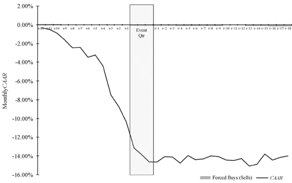
In Chapter 3 I analyze the behavior of liquidity characteristics of assets around fire sales by mutual funds. Such large liquidity-driven sales result in significant negative price pressure, leading to a temporary drop in the asset price around the sale event. I argue that after the sale is completed the level of asset liquidity should be similar to the level before the sale and the price of the asset should return to its intrinsic value. Yet, in the empirical literature investigating fire sales, observed return reversals on av-erage last over 18 months. Such long return reversals could be caused by a permanent drop in asset liquidity after the fire sale, as agents might consider a liquid pre-sale asset to be less liquid after the sale. Such behavior would result in the asset actually being less liquid, because, if it is traded less frequently after the sale, its bid-ask spread would increase, which increases the assets’ transaction cost. In order to answer this question, I compare the behavior of asset-liquidity characteristics for large liquidity and value-driven sales by mutual funds. Additionally, I look for evi-dence of liquidity provision and measure the profitability of such a liquidity provision strategy after fire-sales.

(13)

1 The Cost of Funding Flow

Corre-lation

1.1 Introduction

In this chapter I investigate how correlation between funding flows (or liquidity shocks) of investors that hold overlapping port-folios can destroy wealth. Correlated funding flows lead to com-monality in trading by investors, which can create significant price pressure if this trading is concentrated on the same set of assets. Additionally, as such price pressure can be positive or negative it makes investors incur trading cost when buying as well when as selling assets. In this study I focus on trading by mutual funds, since, by construction, they must make liquidity driven trades matching their capital in- and outflows. Moreover, mutual funds typically specialize in trading particular portfolios (such as industry specific stocks for example) and therefore are inclined to hold overlapping portfolios with peer funds. Finally, mutual fund flows are highly correlated between funds. Potential losses for funds from simultaneous trading of overlapping port-folios are therefore high. In order to quantify the risk of in-curring such losses I introduce a measure of portfolio-adjusted funding-flow correlation (PFC) and argue that flow correlation should be considered by fund managers in their portfolio choice. I show empirically that if flow-induced trading is contemporane-ously positively correlated with cumulative flow-induced trading (and therefore price pressure) of a fund’s portfolio, this leads to destruction of fund investors’ wealth.

(16)

and is it economically significant? What proportion of funds se-lect their portfolios optimally with regard to flow correlation?

The standard assumptions in financial economics are that agents have either independent and identically distributed (i.i.d.) trading/liquidity needs or that they are not liquidity constrained at all and trade at their own discretion. Either assumption means that, trading patterns are not correlated between agents and can be completely ignored when setting up the portfolio choice prob-lem. In this paper I argue that, once systematic liquidity needs - or correlation in liquidity needs between agents - is introduced, optimal portfolio weights become conditional on the contempo-raneous trading needs of an agent with respect to others. Sys-tematic liquidity shocks can create sysSys-tematic up- and down-ward price pressure on certain assets, so an agent whose liquid-ity needs are positively correlated with such systematic shock-induced price movements will have lower expected utility from holding this particular asset compared to an agent whose trading needs are not correlated with the systematic shock which aﬀects the asset price.

In this study I investigate the case of mutual funds with cor-related funding flows. It has been shown that capital flows in and out of mutual funds and the resulting flow-induced trading can create significant price pressure on individual stocks and the mar-ket portfolio1_{. Mutual fund flows are not necessarily correlated} with the fundamentals of the assets held by the fund, though it has been shown empirically that mutual fund flows are cor-related with lagged returns2_{. The correlation examined here is} between mutual fund flows and the cumulative price pressure in their portfolio due to flow-induced trading by peers. While the eﬀect of price pressure from flow-induced trading on the

perfor-1_{See Coval and Staﬀord (2007), Ben-Rephael, Kandel and Wohl (2011),}

Edelen and Warner (2001), etc.

(17)

mance of assets has been well documented in previous studies3_{, I} mainly investigate the eﬀect of correlated trading on the perfor-mance of the fund itself, not on the asset price. Basically, a fund with positively correlated trading needs with his peers systemat-ically sells too cheap and buys too high4_{. The study most closely} related to this chapter is Lou (2010) who calculates a measure of expected flow induced price pressure of fund portfolios, but does not account for the trading dynamics of funds5_{. The PFC} measure I introduce here expands the idea of flow induced price pressure by defining expected costs conditional on the contempo-raneous trading needs between peers.

My results can be summarized as follows. In the theoreti-cal part of this work, I first illustrate that correlation between mutual fund flows and aggregate value weighted portfolio flows becomes an important variable in choosing the optimal portfolio. I derive this result by formally describing the maximization prob-lem of mutual funds when faced with liquidity driven transaction cost. I further demonstrate that a systematic component in the flows of holders of an asset will decrease the asset price and in-crease unconditional expected returns. Finally, I derive an upper bound of optimal portfolio (or asset) flow correlation conditional on the fund. Empirically, I estimate the determinants of flow correlation in fund portfolios and find that correlation is higher for funds with high past excess returns and high loads on risk factors. Moreover, correlation increases with portfolio concentra-tion and for less liquid portfolios. Next, I find significant evidence that flow correlation decreases fund excess returns in the long run, when controlling for fund style. I find that high-correlation funds underperform similar low-correlation funds on average by

3_{For example: Coval and Staﬀord (2007), Frazzini and Lamont (2008) or}

Koch, Ruenzi and Starks (2009)

4_{Greene and Hodges (2001) show that active trading of open-ended funds}

has a meaningful negative economic impact on the returns of passive, non-trading shareholders. Here, I argue that once considering flow correlation such a dilution eﬀect on long horizon fund investors may be exacerbated.

(18)

1.4% annually. Finally, I show empirically that around one third of funds holds non-optimal portfolios with excess flow correlation. The rest of the chapter is structured as follows. In Section 1.2 I describe the contribution of this paper to existing literature. Section 1.3 explains the theoretical background, while Section 1.4 outlines the sample selection process. Section 1.5 describes the construction and properties of the flow correlation measure, Section 1.6 outlines the empirical results and Section 1.7 con-cludes.

1.2 Contribution to existing literature

This work is related to three distinct strands of literature, in particular, the eﬀect of mutual fund flows on assets, mutual fund performance and optimal deviation in portfolio choice. Below, some of the most closely related papers are described in context with the contribution of this chapter. Nevertheless, as these are broad categories of research I do neither attempt to list nor re-view the cross-section of available literature, but merely mention a few representative and relevant examples.

(19)

fund managers to sell assets at fire sale prices. Asset prices later recover and the mutual fund forgoes this positive return. As mentioned above, Frazzini and Lamont (2008) argue that mutual fund investors make bad decisions by investing into segments with high past returns, therefore driving up the current price over its fair value. Such liquidity driven excess returns are subsequently destroyed when prices return to the fundamental level and in-vestors begin to withdraw their moneys. The ”dumb money” argument is that it is optimal to invest against the general flow of funds. I relate to this argument by showing that mutual fund managers should consider correlation with peers’ funds trading when selecting their portfolio, hence avoiding buying overpriced assets alongside everyone else. Koch et al. (2009) document that commonality in liquidity of investors with similar holdings and trading patterns cause commonality in asset liquidity and use mutual funds flows to proxy for investors’ liquidity needs. Sim-ilarly, Anton and Polk (2012) show that common ownership by mutual funds causes excess co-movement in asset returns. They explain this as a result of commonality in liquidity due to flows, but instead of using flows they look at shared ownership. I add to these papers by arguing that fund managers should be able to outperform their peers by adjusting portfolios for flow corre-lation. I estimate that commonality in liquidity of investors with similar holdings and trading patterns cause commonality in asset liquidity and use mutual funds flows to proxy trading patterns. Furthermore, this work highlights the relationship between com-monality in flow driven funding liquidity and asset prices as well as fund returns.

(20)

(21)

Ad-ditional related fund performance literature includes the ”Smart Money Eﬀect” documented by Gruber (1996) and Zheng (1999) who indicate that funds receiving flows subsequently outperform in the short run. They estimate a significant eﬀect especially for smaller funds. Similar to Lou (2010), I argue that such short run outperformance may be caused by simultaneous trading of overlapping portfolios and that such excess returns are destroyed by increased liquidation costs in the long-run.

(22)

exhibit outflows. This complicates a manager’s portfolio choice somewhat, as a fund cannot simultaneously hold the same ”win-ning” portfolio and have uncorrelated flows with the other hold-ers of the same portfolio. Therefore, similar to Wagner’s result, I argue that there must exist an optimal level of deviation that maximizes return while minimizing expected cost from liquidity induced trading.

The main contribution of this chapter to existing literature is to show that contemporaneously correlated trading flows and especially portfolio-adjusted funding-flow correlation (PFC) are important parameters in portfolio choice and that they have eco-nomic significance in mutual fund performance. Furthermore, I assess to which extent mutual fund managers take PFC into ac-count and if the mutual fund market is competitive once flow correlation is considered, i.e. if flow correlation is a variable from which mutual fund returns can be predicted.

1.3 Theoretical Motivation

A simple example

To illustrate how systematic wealth shocks can influence portfolio choice with a simple example, let us assume a worker who receives the majority of his wealth as labor income from a particular firm and his income is at least partially stochastically linked to the firms performance. The worker now wants to invest his wealth. I argue that for this particular worker, an investment into shares of the employer firm is a relatively bad investment decision6_{. When} buying shares of the firm, the worker’s investment returns are automatically positively correlated with his income stream. This means, during good times (when the firm does well), he is likely to receive an extra bonus or a salary raise, while simultaneously getting high returns from his stock investment. Whereas, during

(23)

bad times he is likely to earn less or even loose his job, while his investment also yields low returns. On the other hand, an agent who has an i.i.d. income stream in relation to the perfor-mance of the firm will consider the firms stock a relatively better investment in comparison. Basically, the worker’s set of stochas-tic discount factors are partially defined by his stochasstochas-tic income stream. Hence, for low-income states of nature his marginal util-ity of wealth is greater, and so is the respective stochastic dis-count factor. Therefore, correlation between his set of stochastic discount factors and the payoﬀ of the firm’s stock is lower com-pared to an agent with i.i.d wealth. Such lower correlation leads to a lower price this particular worker is willing to pay for the stock. Additionally, the worker is more likely to be forced to liq-uidate his stock holdings in the bad state, at a low price, while he may invest excess cash in the good state, at a high price, which reduces his expected realized return on the asset. This simple example illustrates that correlation between income, or liquidity, with asset payoﬀs matters when choosing an investment portfolio.

But, asset returns are not only driven by fundamentals, also liquidity or non-information based trading moves the price of an asset. So, when there is a systematic component in the wealth shocks of constrained agents who trade a particular asset in or-der to satisfy their liquidity needs, they will cumulatively exert price pressure on the asset due to simultaneous trading. Hence, an agent whose wealth shocks are correlated with the cumulative price pressure from liquidity trading (and therefore are corre-lated with the wealth shocks of the other holders of the asset) faces a similar problem than the worker described in the example above, even with shocks being completely independent from as-set fundamentals7_{. The portfolio choice problem described below} formalizes this problem.

7_{Assuming there is no correlation between the particular stock’s}

(24)

Portfolio Choice Problem of Mutual Funds with

Flow Correlation and Trading Cost

Let there exist I funds (agents)8 _i _{= 1}_{. . . I} _{that invest in} port-folios of assets n = 1. . . N with ωi,n,t portfolio weights. Each

fund is subject to exogenous cash inflows and withdrawals (liq-uidity shocks) by its investors at the end of each period. Let

F lowi,t represent inflows (withdrawals for values<0) into (from)

fund i at time t. For simplicity let us assume future fund flows to be unexpected flows9_{, so} _Et_[_{F low}

i,t+1] = 0 ∀i. Moreover, I

assume that flows have stochastic variance E[σF low] =constant,

V ar[σF low] > 0. Finally, let us assume flows to be uncorrelated

with fundamental asset returns. The stochastic variance term is used to model uncertainty about fluctuations in liquidity10 11_.

Since funds must be seen as conduits - they do not own or hold a large amount in cash, but buy and sell assets with their investors’ capital - an inflow or outflow of capital has an eﬀect on their portfolio. In case of an outflow - investors taking money out of the fund - a portion of the fund’s portfolio must be sold. When a fund receives an inflow of capital it has to invest this money and

8_{Assuming a suﬃciently large} _I _{so individual funds can be considered}

marginal price takers.

9_{Empirically, mutual fund flows exhibit high first-order autocorrelation}

and correlation with the fund’s lagged performance, which makes it possible to predict flows at least partially. However, a large part of mutual fund flows remains unpredictable. Arguably, the more interesting part of flows are unexpected flows as far as liquidity is concerned. In any case, it should be considered that funds are not able to react ex-ante even to expected flows, since they i.e. cannot short sell or borrow. I therefore perform the empirical analysis in this paper using total net flows and not just unexpected flows, while, for simplicity, assuming flows to be unexpected in this theoretical section.

10_{In this dynamic setup the absolute level of liquidity does not matter,}

the expectation of volatility in aggregate liquidity is important for expected returns and the stochastic variance enters similar to a jensen’s inequality term

11_{I do not assume Flow to be normally distributed, but require normal}

(25)

typically would scale up its portfolio12_{. One can easily calculate} the aggregate amount of each asset n that should be bought or sold by funds at timet, were they all to simply expand or reduce their portfolios to match flows while keeping portfolio weights constant. Letδi,n,t be the weights of the trading portfolio13. The

aggregate traded amount of each asset is calculated as:

AF lown,t= I �

i=1

δi,n,tF lowi,t

where�N_n₌₁δi,n,t= 1 for all funds i= 1. . . I.

When aggregating expected flows it holds that the expectation of the size of the aggregate trade in the next period is zero, so

Et_[_{AF low}

n,t+1] = 0. Since portfolio weights ωi,n,t are the

opti-mal weights at time t it follows that Et₍_δ

i,n,t+1) = ωi,n,t. When

actually trading at t+1, fund managers choose the actualδi,n,t+1 trading portfolio weights14_.

Next, I model liquidation cost c(_·) as a function of the ag-gregate transaction for each asset at t. For simplicity let us assume it to be a linear function of the form c(AF lown,t) =

a+ b _· (�I_i₌₁δi,n,tF lowi,t) and set a = 0, ignoring fixed

trad-ing costs. Hence, all assets can be traded costless in very small

12_{Liquidity considerations aside, the amount of money managed by the}

fund should not change its portfolio choice. For a discussion see Bhushan (1992). Furthermore, empirical evidence in support of scaling has been pre-sented by Lou (2010).

13_{Defined as:} _δ

i,n,t =ωi,n,t+ (ωi,n,t−ωi,n,t−1)_{F lowi,t}Wi,t−1 since it must hold

that δi,n,tF lowi,t = ωi,n,tWi,t−ωi,n,t−1Wi,t−1. For zero flows the trading

portfolio does not exist and trading portfolio weights are undefined.

14_{There are 3 distinct cases: For} _ω

i,n,t = δi,n,t+1 the portfolio weight

does not change, the fund is simply scaling up/down its previous position.

For ωi,n,t > δi,n,t+1 the fund trades less of asset n than in the case of

scaling. With positive (negative)F lowi,t+1this means that the fund reduces

(expands) its relative position in the asset. For ωi,n,t < δi,n,t+1 the fund

trades more of assetnthan in the case of scaling. With positive (negative)

F lowi,t+1 this means that the fund expands (reduces) its relative position

(26)

quantities, while only aggregate volume has an eﬀect on the cost of trading. The multiplierb can be understood as indicating the absolute value of liquidity-trading driven return per $ volume traded, similar to the Amihud-measure of an asset15. Depending on the sign of AF lown,t,c(·) can be positive or negative. In this

framework a ”negative cost” can be understood as an additional return rewarding provision of liquidity.

So, realized returns on asset n consist of 2 components; the return rn,t from the fundamental value of the asset, minus the

cost of trading c, both to be realized at the end of each period. If a fund does not trade a particular asset, it realizes only its fundamental returnrn,t as it keeps holding the asset in the

port-folio and I assume that the asset price returns to its fundamental value after everyone has traded. For each unit of the asset traded the fund realizes rn,t- c(·). This incurred trading cost then gets

diluted over the entire position, so even fund-investors that have not caused outflows suﬀer as their share of the fund looses value due to the dilution of cost16_.

I model the portfolio choice as a pure investment problem in-corporating the above described transaction cost from stochastic flow induced trading17_{. Each fund} _i _{maximizes expected utility} of its investors over their future wealth according to the following maximization problem:

max

ωi,1...N,t

EtU �

Wi,(t+1)

�

=

15_{To simplify the theoretical setup I assume} _b _{to be constant across all}

assets. A nice extension of this model would be to allow for an endogenous

bn as this way liquidity cost would be determined by portfolio choice and

correlation in flows.

16_{This actually might cause a type of ”run” on the fund in the spirit of}

Bernardo and Welch (2004) when fund investors expect a significant mass of others to redeem their share in the fund.

17_{I assume that there are no conflicts of interest between fund-managers}

(27)

= max

ωi,1...N,t

EtU � _N

�

n=1

�

ωi,n,t(1+rn)−δi,n,(t+1)F lowi,(t+1)c(AF lown,(t+1))

��

(1.1)

s.t. �N_n₌₁ωi,n,t= 1, ωi,n,t ≥0, ∀i, n, t

Short selling is restricted and funds have to invest their en-tire capital into the portfolio. Each fund’s initial wealth under management is normalized to 1. Flows have to be seen as fund investors moving money between their cash holdings and their mutual fund portfolios, so they are not added or subtracted from wealth in the maximization problem. There exists a riskfree asset with return r that can be traded costless. The cost component in equation (1.1) is calculated by the cost function c(_·) that de-pends on the aggregate volume of asset n traded by all funds in the market, multiplied byδi,n,t+1F lowi,t+1, which is the dollar

amount of assetn traded by fundiatt+ 1. This equals the total liquidity loss (gain) in dollar terms at time t+ 1, since the loss (gain) from the trade gets diluted over the entire position. This, as wealth is normalized to 1, equals the portfolio weighted re-turn of the position. Using iterated expectations we can replace

δi,n,t+1F lowi,t+1 with ωi,n,tF lowi,t+1.

The N first order conditions of equation (1.1) for each fund i

yield:

E�U�(Wi,t+1)[(1 +rn)−F lowi,t+1c(AF lown,t+1)] �

= =E[U�(Wi,t+1)(1 +r)]

(28)

asset n is18_:

E[ ˜Ri,n] =

= E[rn−F lowi,(t+1)cn,(t+1)(AF lown,(t+1))−r] = (1.2) = ₋E[U

��₍_W

i,(t+1))]

E[U�₍_W_i,₍_t_+1))]Cov(Wi,(t+1), rn) + (1.3)

+ E[U

��₍_W

i,(t+1))]

E[U�₍_W_i,₍_t_+1))]Cov

�

Wi,(t+1), F lowi,(t+1)c(AF lown,(t+1)) �

Equation (1.2), when using the linearity assumption for the shape of the cost function c, yields:

E[ ˜Ri,n] =E[rn−r]−bCov(F lowi, AF lown) (1.4)

Equations (1.3) and (1.4) show the conditional expectation of fundifor the realized excess return ˜R on assetn. Note that this is not a pricing equation as I have not imposed market clearing so far. It is merely the expected realized return conditional on the contemporaneous trading pattern of fundi. When averaging across assets (1.4) the expected realized excess portfolio return of fundi becomes:

E[ ˜Ri] = N �

n=1

ωi,n �

E[rn−r] �

−E�bCov(F lowi, P F lowi) �

(1.5) where portfolio level flow for fundi is calculated as:

P F lowi = N �

n=1

ωi,nAF lown

Aggregating equation (1.3) across agents and averaging across assets yields the unconditional expectation of the realized excess return on the market portfolio for the average fund.:

E[ ˜Rm] = E[rm−r−bσM F low2 ] = (1.6)

= −E

i_[_U��₍_W

m,(t+1))]

Ei_[_U�₍_W_m,₍_t_+1))]σ

2

rm+ +E

i_[_U��₍_W

m,(t+1))]

Ei_[_U�₍_W

m,(t+1))]

b2V ar(σ_{M F low}2 )

18_Using: _E_{[ ˜}_A_B_˜_]

− E[ ˜A]E[ ˜B] = Cov( ˜A,B˜) and Cov(f(˜x),y˜) =

(29)

It can be seen that if there are many funds with i.i.d. flows, the variance of the aggregate flow in the market M F low will be zero in the limit as liquidity trades of individual funds cancel each other out. Traders on average will realize simply the fundamental market return r∗

m. As soon as trading shows some systematic

component across fund flows, the variance term becomes positive and realized returns on trading the market portfolio are reduced, on average, by the variance multiplied with the sensitivity of stock returns to volume. For each stock n the unconditional realized return for the average trader is:

E[ ˜Rn] = E[rn−r−bσAF low2 n] = (1.7) = �E[rm−r−bσM F low2 ]

�� Cov(rm, rn)

σ2

rm−b

2_{V ar}₍_σ2

M F low)

−

−b

2_Cov₍_σ2

AF lown, σ 2

M F low)

σ2

rm−b

2_{V ar}₍_σ2

M F low) �

When summing across agents I implicitly assume market clear-ing, so the above becomes a pricing formula determining the fun-damental return rn, which will be diﬀerent from r∗n in the case

with no aggregate flow variation. The first notable fact is that the market risk premium is smaller than without liquidity trad-ing cost19_{. Next, we see that expected realized returns decrease} in commonality of the liquidity risk fromAF low with respect to market liquidity risk M F low. Finally, investors demand a pre-mium of bσ2

AF lown to be compensated for the expected loss from trading.

Agents with negative flow correlation to the aggregate flow of an asset will realize additional positive returns over the fun-damental return. Yet, if these agents are funding constrained they cannot absorb all the liquidity risk, otherwise they would smooth out aggregate flows until the variance ofAF lownbecomes

zero and expected returns equal expected no-flow fundamental re-turns r∗

n. In equilibrium, the price of asset n has to decrease, so

19_{This result is in line with Jacoby, Fowler and Gottesman (2000), who}

(30)

E[rn −r] > E[r∗n−r]. The expected realized excess return for

the average agent with i.i.d. trading pattern is greater or equal to the return in the equilibrium without losses from systematic liquidity trading, so the expected fundamental return of the asset has increased. The important result obtained here is that asset prices are related to the systematic component of trading needs of the current holders of the asset.

This result is fundamentally diﬀerent from liquidity capital asset pricing models (LCAPM) such as the pricing model intro-duced by Pastor and Stambaugh (2003). In the LCAPM ap-proach the level of market liquidity is considered a priced risk factor and investors are rewarded for diﬀerent types of correla-tion between the (fundamental) return of an asset and the re-spective liquidity factor. So, for example, an asset which yields high returns in a low-liquidity state of nature will be priced at a premium in the LCAPM. In contrast in the model described here, no priced liquidity market factor exists. Agents demand a premium to hold assets, which are currently held by an investor group whose aggregate flow has an expected non-zero variance. Nevertheless, agents are only able to demand such premium if the variance in the aggregate flow is specific to the asset. The second covariance term on the right hand side of Equation 1.7 reduces the premium that can be demanded for aggregate flow variance risk if such risk is correlated to market-level variance in flows. This means basically that an investor is not compensated for ag-gregate liquidity risk in the market. Meanwhile, the investor can demand a premium for holding an asset whose aggregate investor flow risk exceeds the risk of flow variation in the market.

Assuming market clearing and equilibrium pricing as outlined above, let us look again at Equations 1.4 and the left hand side of 1.7 and discuss them in the context of the equilibrium price. For example, fund i holding asset n if Cov(F lowi, AF lown) >

σ2

(31)

between its flows and the aggregate portfolio weighted flows of assetn. On the other hand, assets whereCov(F lowi, AF lown)<

σ2

AF lown will yield additional excess returns to the respective fund, since it becomes a relative liquidity provider. A fund should therefore increase its portfolio weights in such assets. From this I infer Cov(F lowi, P F lowi)≤ σP F low2 i to be the upper bound of optimal flow correlation at the portfolio level. Each fund should be able to find a portfolio where the covariance between its flow and the portfolio weighted average flow is at least equal but not greater than the variance of the portfolio flow itself. Nevertheless, as I do not impose a particular underlying flow structure it is not possible to calculate the lower bound, which should be the portfolio that yields the highest excess return due to liquidity provision by the fund and should therefore automatically be the optimal portfolio. Normalizing the upper bound covariance, the respective upper bound correlation coeﬃcient is:

ρF lowi,P F lowi ≤

σP F lowi

σF lowi

(1.8)

A couple of properties should be discussed. First, the lowest possible upper bound is zero, which is the case where individual flows cancel out the aggregate flow and its standard deviation becomes zero. In this case the correlation coeﬃcient also goes to zero. For funds with very small flows the upper bound becomes very large. In this case the fund will not incur much liquidity related losses due to the small size of its liquidity trading even though flow dynamics can be quite highly correlated with ag-gregate flows. A similar upper bound can be derived for each asset/fund combination. It can be expected that a fund will only buy a particular asset for which its correlation exceeds the upper bound if the fund manager believes that the asset is mis-priced and will at least yield an additional expected return of

(32)

Equilibrium

From the above reasoning for the existence of an optimal upper bound one can conject that for each possible variance-covariance matrix of flows there exists at least one corresponding pareto-optimal equilibrium allocation with regard to losses from par-allel trading. This equilibrium is achieved once all agents ad-just their portfolios to remain below the optimal upper bound. The upper bound of one agent is aﬀected by the portfolio choice of the other agents with whom he has non-zero funding flow correlation. In the case where all agents hold portfolios with

ρF lowi,P F lowi ≤

σ_{P F lowi}

σ_{F lowi} the upper and lower bounds converge and

become equal to the agents’ portfolio-adjusted flow correlation coefficient ρF lowi,P F lowi. This is due to the fact that if all agents hold portfolios where they do not make losses from to simultane-ous trading beyond the level that is priced in the market other agents can not achieve additional gains from contemporaneously providing liquidity to their peers. Hence, the upper and lower bounds converge, a pareto improvement becomes impossible and a pareto optimal equilibrium is achieved. Once all agents hold such portfolios, for any additional agent entering this economy a portfolio-indifference result holds, similar to the equilibrium result outlined in Wagner (2008). Each portfolio gives the same expected return after cost from simultaneous trading is taken into account. In the equilibrium described above, all portfolios must give the same level of expected utility, since otherwise investors holding portfolios with lower utility would switch. Therefore, in such an equilibrium, a new - price-taking - investor is indifferent between portfolios, regardless of his or her fund flow correlation with others20_.

20_{This argument purely concerns portfolio returns regarding losses from}

(33)

Empirical Tests

In this paper I do not test the asset pricing implications of the model described above, but am rather interested in the impact of flow correlation on mutual fund performance as described in Equation 1.4. I introduce a measure of portfolio-adjusted flow correlation (PFC), representing the covariance term of Equation 1.4 and test if there is a negative relationship between expected risk-adjusted returns of a fund and its level of PFC. Furthermore, I test if fund managers hold non-optimal portfolios with respect to the theoretical optimal upper bound of flow correlation derived above. For future work it would be interesting to directly test the asset pricing and equilibrium implications of the model with respect to correlation in trading needs.

1.4 Data and Sample Selection

In this study I use 3 distinct databases, namely the CRSP Sur-vivorship Bias Free Mutual Fund database, the CDA/Spectrum Mutual Fund and Investment Company Common Stock Hold-ings Database provided by Thompson Reuters, and the CRSP database on common US stocks. The sample being used spans the period January 1990 to December 200821_.

The CRSP Mutual Fund database contains monthly informa-tion about funds’ total net assets under management (T N A), fund returns, equity ratios and cash holdings for each share-class of the fund. Monthly fund-returns reported in CRSP are net re-turns, after fees etc., but before any front-end or back-end loads. Following standard literature, I assume implicitly that funds’ flows occur at the end of each month, so I calculate monthly flows in and out of funds aggregated to fund level as:

F LOWi,t =T N Ai,t −T N Ai,t−1∗(1 +ri,t)

21_{For the period 1980-1989 quarterly data of flows is available, but I do}

(34)

where T N Ai,t are total net assets held by fund i at time t and

fundi�s returnsri,t are returns realized in period [t−1, t]. I

cor-rect for mergers, subtracting the final T N A of the dying fund from the F LOW of the surviving fund during the month of the merger. Since information about merger dates in CRSP is not very precise I use a matching procedure to select the month with the highest flow at the acquiring fund as the true month of the merger within a 6-month window [t₋1, t+5] around the reported merger date. Subsequently, as I am interested in the analysis of correlation of flows, I delete the first and last flow observation for each fund. These flows are equal to the initial and finalT N A of a fund, and since funds initiate and terminate at random times their initial and final flows are not correlated with flows of their peer funds. Additionally, I correct the database for obvious digit entry errors of total net assets by using a procedure to identify subsequent inflows and outflows of the same order but reversed sign due to an outlier inT N Aof an order of magnitude of 10 (or 0.1) compared with previous and subsequent T N A values. To avoid removal of correct entries by this procedure I check if the absolute value of the calculated flow created by the erroneous

T N A observation is at least 3 standard deviations away from

the funds’ flow average in order for the erroneous T N A to be removed. The above described procedure and merger correction appear to eliminate almost all of the extreme outliers in the flow distribution. In order to address issues regarding fund incubation bias, I exclude the first 12-month fund returns22_{, which also} ad-dresses any concerns that new funds might be cross-subsidized by their respective fund families23_{. I further winsorize the dataset} by deleting merely the 0.1% and 99.9% extreme tails. Finally, I only include funds with minimum T N Aof 1M$ in the sample.

Thompson Reuters’ CDA/Spectrum Mutual Fund database contains data on mutual fund portfolio holdings. The reporting

(35)

frequency is quarterly for most funds in the sample. Since CDA bases its information on the holdings file date, and not the actual reporting date, for which the holdings are valid, I correct stock prices and adjust for eventual stock-splits between reporting and file date. Finally, I merge CRSP and CDA using the MFLINKS tables provided by Wharton Research Data Services (WRDS). As the CDA database reports holdings on fund level, not by fund share class, I consolidate CRSP share classes to fund level using the MFLINKS merging table. Fund level returns are calculated as share-class returns value weighted by the TNA of each class, fund level total net assets are the sum of assets of each under-lying share-class. To ensure correct mapping I require that the TNA’s reported by CRSP and Thompson for each fund do not diﬀer by more that a factor 2 (0.5). Following Lou (2010) I only include US domestic equity mutual funds in the sample, in or-der to obtain comparable results. I therefore include funds with CDA/Spectrum investment objective code specified as aggres-sive growth, growth, growth and income, balanced, unclassified or missing. Furthermore, I restrict the sample to funds with an equity ratio between 0.75 and 1.224_{. Table A.2 in the Appendix} provides the summary statistics of the merged sample.

Data on monthly share prices and returns, bid-ask spreads, volume and shares outstanding is obtained from the CRSP Com-mon Stock Holdings database. I exclude stocks priced below $5, as is common practice in order to avoid microstructure noise. Furthermore, I employ the three Fama-French risk factors and the momentum factor, all provided by Prof. Kenneth French, to calculate fund- and portfolio alphas using 48-month rolling windows. Additionally, I calculate the monthly Amihud liquid-ity measure25 _{for each stock using a 48-month rolling window.} The relative Bid-Ask spread is computed as bid-price minus ask-price divided by the mid-ask-price. Finally, I calculate the normalized

(36)

monthly Herfindahl Index of portfolio concentration for each fund as:

Hi,t = Ni

�

n=1

ω2_i,n

H_i,t∗ = H−1/Ni 1₋1/Ni

1.5 Portfolio-Adjusted Flow

Correla-tion Measure (PFC)

It has been shown that flow induced trading by mutual funds creates price pressure on individual stocks. Coval and Staﬀord (2007) show that extreme fund flows lead to significant drops in share prices, while Lou (2010) shows that price pressure from flow induced trading is predictable on a stock level. Here I create a correlation measure that allows a fund to know its exposure to simultaneous flow induced trading by peer funds. In partic-ular, I construct a measure of correlation between the flows of an individual base fund and the portfolio weighted sum of flows of its peer funds holding overlapping positions. Basically, a fund manager that does not buy or sell assets should not be concerned about price variation in her portfolio due to other funds’ flow induced trading. Price drops due to peer funds’ liquidity trading today mean higher returns tomorrow, as there is no change to assets’ fundamentals. A problem arises if said fund manager is forced to sell assets due to withdrawals from her fund while the asset price is depressed. Equally, a fund benefits greatly from inflows if it is able to buy assets cheap, while other funds are forced to sell them.

(37)

should not be exceeded in order to avoid costs from simultaneous liquidation. A fund manager should therefore rebalance her port-folio by decreasing holdings of assets which lead to exceedance of this bound. The PFC measure is the portfolio-adjusted flow correlation that can be compared against the upper bound at the fund portfolio level.

The idea behind the PFC measure constructed here is to have an indicator for the level of flow induced unidirectional contem-poraneous trading by peer funds inherent in fund portfolios. In a way, choosing a portfolio with a certain flow correlation means choosing a level of liquidity timing. A manager holding a high PFC portfolio exhibits negative timing, so she would systemati-cally sell cheap and buy expensive. A zero PFC portfolio would mean no liquidity timing, in this case assets are bought and sold - on average - at their fair value, as far as mis-pricing due to flow induced trading is concerned. Negative PFC is equivalent to a manager who possesses positive liquidity timing ability, where assets are being bought cheap and sold expensive as the fund provides liquidity to its peers.

To construct the PFC, I first calculate the aggregate amount of each asset n that should be bought or sold by funds at time

t, were all funds to simply expand or reduce their portfolios to match flows while keeping portfolio weights constant. Mutual funds typically scale their portfolios up and down with inflows and redemptions (see e.g. Bhushan (1992)). Lou (2010) estimates a partial scaling factor to be 0.97 for outflows and 0.62 for inflows. This means that funds facing redemptions almost perfectly scale down their portfolios, while with inflows on average 62 cents per Dollar gets invested into the existing portfolio. In a first stage, assuming near-perfect scaling, I construct backward looking 48-month rolling windows for each asset, summing the flows of all fund’s currently holding the asset26 _{multiplied with the current}

(38)

portfolio weights in each fund’s portfolio.

AF LOWn,t,[t..t−47] =

I �

i=1

ωi,n,t∗F LOWi,[t..t−47]

This leads to 1.331.781 distinct 48-month asset-level flow win-dows. As a second step, I aggregate the asset flow windows into portfolio flow windows for each fund-month observation, weigh-ing the asset flows with the current portfolio weights of each base fund.

P F LOWi,t,[t..t−47] =

N �

n=1

ωi,n,t∗AF LOWn,t,[t..t−47]

Finally, I calculate the correlation coeﬃcient between the aggre-gate portfolio flow window and the corresponding 48-month fund flow window for each fund/month observation, given an existing 48 month flow history for the base fund.

ρi,t =

Cov(P F LOWi,t,[t..t−47], F LOWi,[t..t−47]) σP F LOWi,t,[t..t−47]σF LOWi,[t..t−47]

From the before mentioned sample I end up with 163,642 fund-month estimates of the PFC.

By way of construction, I expect the PFC to systematically underestimate the real absolute value of correlation. This is due to the fact that not all funds currently holding an asset have a flow history of up to 48 months. So, when adding up flows with cur-rent portfolio weights, peer funds with a flow history shorter that 48 months are underweighted in the correlation measure. Never-theless, excluding funds with shorter flow history might distort the measure even more, since more recent flows are more indica-tive. Reducing the length of the estimation window mitigates this problem, while at the same time adding to the estimation error in the correlation measure. As a robustness check I have run are value weighted past flows [t..t−47] of the funds holding the asset at time

(39)

the analysis using shorter 24 and 12 month estimation windows, obtaining largely consistent results. As this problem supposedly can only, if anything, weaken my results, I prefer the measure with smaller estimation errors and longer window size and report everything based on 48-month windows, keeping the downward bias in mind when analyzing my results.

The portfolio flows contain the 48-month flow of the base fund itself, which increases the PFC significantly when assets are mostly held by just the one fund. One could, of course, first sub-tract the base fund flow from the portfolio flow, creating portfolio flow windows that only contain weighted peer fund flows, before calculating covariance matrix. Nevertheless, since I am interested in the liquidity management of fund managers, keeping the base fund’s own flow in the portfolio flow gives a clearer picture. If a fund holds a nonoverlapping portfolio of probably smallcap -stocks, then its correlation measure would be positive and close to 1. As there are no other funds trading in these particular stocks, the fund will face a significant price discount when trying to wind down its position. Hence, it is subject to its own flows inducing price pressure.

(40)

1.6 Empirical Results

Determinants of the PFC Measure

(41)

size-factor strategy and does not invest into very small stocks. The load on the value-HML factor is centered around 0.0 but with a relatively large standard deviation. On the other hand, momen-tum appears much more narrowly centered around 0.0, so not many funds actually appear to be actively trading pure momen-tum or contrarian strategies.

Next, I analyze the determinants of PFC (ρi,t) at the

port-folio level. Portport-folio and fund characteristics are expected to influence the level of flow correlation, yet if there is large unex-plained variability, this would mean that the fund manager has certain freedom to manage the level of flow correlation. I run the following regression to determine which factors influence flow correlation:

ρi,t = α+β1BM KT,i,t+β2BSM B,i,t+β3BHM L,i,t+β4BM OM,i,t

+β5Log(Amii,t) +β6Log(Herfi,t) +β7Agei,t

+β8SampleM ontht+β9Lag(ExRet)i,(t−1)+�i,t

Table A.4 reports the determinants of the PFC measure as results of pooled-OLS27 _{regressions using the 3 Fama-French and} the momentum factor loads as well as the Amihud measure of portfolio liquidity, the Herfindahl index of portfolio concentra-tion, the fund’s age is included to account for fund growth effects such as fund’s size28_{, reputation, imitation by peer funds, etc., a} month-index of the sample period to capture fixed time effects and the 1-month lag of the excess return as the fund alpha of a 4-factor Carhart model. The intercept shows the average flow correlation at around 0.28, with a declining time trend, reported by the negative coefficient for the sample month index.

27_{Results are robust to using a Fama-MacBeth approach instead of}

pooled-OLS

28_{It might be prudent to include size as a regressor, which should be}

(42)

Load on the SMB factor is positive and significant, with a coefficient of around 0.15. The higher the load on the factor, the higher is flow correlation. This confirms expectations, as funds following the same investment strategy are bound to hold overlap-ping portfolios while having high correlation in their flows, such as is the case with the size factor coefficient. Nevertheless, the Book to Market Value HML factor and the Momentum factor do not appear to be significantly correlated with the PFC measure. After examining the reason for the weak relationship between flow correlation and these risk and momentum factors, I find that for funds with high factor loads (factor tracking funds), the respec-tive factor load becomes highly significant as a determinant of flow correlation. The last column of Table A.4 reports regression results for funds with dummy variables for high risk factor loads, one standard deviation or more above the average. When con-ditioning on extreme loads for the size factor nothing changes in relation to the unconditional regression specification. But, both the HML-value and momentum factor loads significantly affect flow correlation for funds whose returns are strongly determined by the respective factor. Adjusted R2 _{increases to up to 9.4%.} In the related study of Frazzini and Lamont (2008) they show that their flow based measure of investor sentiment is highly cor-related to the value factor, reporting positive flows into mutual funds that own growth stocks and out of funds that own value stocks. They argue that this investment pattern is not only non-rational but also destroys wealth of mutual fund investors. It is reasonable to assume that investor sentiment causes the higher flow correlation observed for funds with high factor load. Finally, the coefficient for the market risk factor is positive and significant but very close to zero in the regression model without high-factor load dummies. When including the dummies the market risk fac-tor coefficient becomes negative and significant, but remains close to zero.

(43)

co-eﬃcient for the Amihud-measure is positive and significant. A high Amihud-measure means larger price movement per dollar traded. This is bad news for investors as it exacerbates losses from simultaneous trading. The coeﬃcient for portfolio concen-tration using the logarithm of the adjusted Herfindahl index is also significant. This means, the more concentrated the port-folio is, the higher is the flow correlation exposure to the fund. This has been expected, since a less diversified fund is bound to have higher correlation. Flow correlation increases by 0.06 for each increase by one-standard deviation in log(Herfindahl). The Herfindahl index appears to have the highest explanatory power in this regression model. Furthermore, correlation very slightly increases with the age of the fund.

Finally, I find a significant relationship between the cumula-tive past 12-month fund alpha and flow correlation. A posicumula-tive alpha is a strong signal which attracts investment inflows, addi-tionally funds holding such ”winning” portfolios are unlikely to rebalance their holdings. Peer-funds with available funds/inflows are likely to imitate and to tilt their portfolios towards the ”win-ning” portfolio. Both leads to an increase in PFC. Equally, fund holding a ”loosing” portfolio with strongly negative past alpha are likely to have simultaneous outflows, yet, they will rebalance their portfolios away from the ”loosing” portfolio, so their PFC level will drop. So, to summarize, investors chasing past returns, creates flow correlation.

(44)

choose to invest into a particular factor will have less freedom in choosing their portfolio with respect to adjusting for high flow correlation. Moreover, less liquid, more concentrated portfolios seem to be held with higher flow correlation. While in future ver-sions of this work the regression model should include additional measures such as turnover ratio, expense ratio, idiosyncratic risk and size for completeness, the main result here is to show that the explanatory power of a model using a fund’s portfolio char-acteristics with respect to flow correlation is low, which means that a fund manager is able to independently control the level flow correlation in his portfolio.

PFC and Investor Return

In this section I analyze the relation between portfolio-adjusted flow correlation and future fund risk-adjusted excess returns. Re-turns are cumulative and are defined as the return in excess of the risk free rate, as well as alpha from 3-factor Fama-French and 4-factor models including momentum. Table A.5 shows the results forming fund decile portfolios sorted by flow correlation. D1 is the portfolio of funds with the lowest, in this case negative, flow correlation coefficient, D5 and D6 are the median portfo-lios29 _{and D10 is the portfolio of funds with the highest level of} flow correlation. The left panel shows the results when re-sorting the cross-section of funds into deciles each month, while in the right panel all fund-month observations have been pooled before constructing decile portfolios. It can be observed that there is no significant unconditional difference between high and low corre-lation portfolios. Nevertheless, the D5 portfolio, which contains funds for which flow correlation with their peers is very close to zero, outperforms both positively and negatively correlated funds. A t-test for difference in means is significant at a 5% level for the 12-month horizon. Theoretically, one could have ex-pected to see a significant difference in returns also between D1

(45)

and D10, but this sorting does not take any additional portfolio characteristics into account. In order to better understand the impact of flow correlation on performance, funds must be com-pared within peer groups with similar investment styles. I use an approach similar to Daniel, Grinblatt, Titman and Wermers (1997), sorting funds into 125 groups by matching them across 3-style quintiles. I define the quintiles by the factor loads on size, value and momentum of fund returns. Then, within each style group, funds are aggregated into decile portfolios according to their level of fundflow-correlation. Table A.6 reports the results for 1, 3, 6 and 12-month out-of-sample cumulative 4-factor excess returns. It can be seen that the average diﬀerence in returns be-tween the top and bottom deciles of flow correlation within each style are not significantly diﬀerent from zero when averaging over the all style groups.

As this result is not in line with the theoretical expectation of monotonically decreasing risk adjusted excess returns with re-spect to flow correlation, I analyzed results on a style-group-level. 71 of the 125 style groups in the sample show a significantly posi-tive difference in cumulaposi-tive excess return for a 12-month horizon at a 5% confidence level, some groups showing annual differences of up to 12.4%. The 19 of the 25 style groups associated with the highest value factor loads show strong, significantly negative differences in returns between deciles for all horizons. Only 8 style groups not associated with high value factor load show a significantly negative difference in returns, while results are not significantly different from zero for the remaining 21 style groups.

(46)

appears to trade heavily on the value factor while the market re-covers. As (internet-)stocks were undervalued after the burst of the bubble, any liquidity related losses from simultaneous trad-ing were compensated by large excess returns driven by funda-mentals. This means that funds with inflows were able to buy undervalued shares, while funds without inflows (and hence with low flow correlation) were loosing out. This period could be a manifestation of a strong ”smart money eﬀect” as described by Gruber (1996) and Zheng (1999). When removing this particular interval from the sample, the observed eﬀect disappears. Never-theless, rather than removing the sample period, I remove the 25 style groups with extremely high loads on the value factor30_.

When averaging over the subsample of 100 styles, it can be seen that funds with lower flow correlation significantly outper-form their high-correlation peers for holding periods of 3-months or longer.The average annual diﬀerence in 4-factor excess returns between funds with high and low flow correlation is 1.43% after fees and expenses but before loads. Moreover, the results in Ta-ble A.6 are robust to splitting the sample into sub-periods.

Additionally, I control for the level of liquidity and portfo-lio concentration, lagged excess returns as well as fund age and fixed time eﬀects. Table A.7 shows the results of the following regression:

cumExReti,(t+12) = α+β1ρi,t +β2Lag(ExRet)i,(t−1) +β3Log(Amii,t) +β4Log(Herfi,t)

+β5Agei,t +β6Log(F undSize)i,t)

+β7SampleM ontht+�i,t

It can be seen that previous results hold, with a negative and sig-nificant regression coeﬃcient of -1.44% for flow correlation,

con-30_{Excluding these high-factor-load funds seems prudent since in the}

(47)

firming its predictive power for out of sample long horizon excess returns. Portfolio concentration is positive and significant, so less diversified managers appear to achieve higher returns com-pared to their more diversified same-style peers. Fund size is not a significant predictor of fund returns once PFC is introduced. Chen, Hong, Huang and Kubik (2002) find that size is a sig-nificant inverse predictor of mutual fund returns and oﬀer two explanations that would lead to an erosion of performance with fund size, namely liquidity and organizational diseconomies. The finding that size is not a significant performance predictor once introducing the PFC measure can be seen as additional evidence supporting their liquidity argument. Adjusted R-square is 7.53%. Results are robust when splitting the sample into 2 sub-periods.

PFC and Portfolio Choice

In this section I examine if funds select their portfolios optimally to stay below the upper bound of portfolio correlation shown in Equation 1.8. The aim is to examine if there is a diﬀerence be-tween funds regarding their portfolio choice with respect to the bound and to estimate the proportion of ”skilled” funds. Table A.8 shows the median upper bound in the sample, the median value by which funds exceed their respective upper bound and the proportion of funds that hold portfolios where the portfolio flow correlation exceeds the theoretical upper bound of optimal portfolio choice. It can be seen that the average proportion of funds exceeding the bound is 31.4%. I estimate exceedance to be significantly higher in the first half of the sample than in the sec-ond half. Moreover, the median distance between the bound and flow correlation has decreased from its highest value of +0.12 in 1994 to -1.36 in 2004. So it appears that funds in the second half of the sample seem to be better at finding portfolios where they also provide liquidity to each other instead of herding towards a single strategy.

(48)

far as dynamic liquidity hedging is concerned. Two possible rea-sons can explain this result. First, these funds ignore flow correla-tion and systematically destroy investor wealth due flow-induced trading. Second, fund-managers believe in their ability to iden-tify priced stocks whose the additional returns due to mis-pricing outweighs losses from flow-induced trading in which case managers would rightly ignore excess levels of PFC.

Extensions

(49)

An additional extension to this chapter could be a breakdown of results for concentrated versus diversified funds as well as liq-uid versus illiqliq-uid portfolios, since it has been shown that both of these parameters highly influence the portfolio flow correlation statistic.

Also, two alternative specifications of the PFC as performance predictor should be investigated and benchmarked against the PFC presented in this work. First, the diﬀerence between the ac-tual level of PFC and the upper-bound should be a better perfor-mance indicator than the absolute level of the PFC. The further the level of PFC is below the bound, the more a fund should gain from liquidity provision, while a fund exceeding the bound means that the fund pays its peers a premium for liquidity. Since the upper-bound depends on the fund portfolio, an certain absolute level of PFC might mean bound exceedance for one fund, while another fund with the same level of PFC may be far below its respective bound. In the work presented here I am controlling for such a problem using a style-matching procedure, but I think that a diﬀerence measure between the bound and PFC would give a more immediate result. A second alternative specification could be using the residuals from the regression of Table A.4 in-stead of the PFC measure. The regression model estimates the level of inherent flow correlation due to portfolio and fund char-acteristics, so the residuals from the regression are a measure of ”voluntary” flow correlation taken by the fund. Since these residuals are orthogonal to portfolio and fund characteristics, it is not necessary to style match funds when using the residuals as performance predictors.

Additional Robustness

(50)

and found that the correlation coeﬃcient between the 2 diﬀerent estimators is extremely high, at 0.93. Considering such a high level of correlation between the two estimators, and the fact that the use of current weights is required by the theoretical moti-vation for the PFC measure, I believe using current weights to be prudent, and all results quoted in this study are based on current portfolio weighting. The main reason for choosing cur-rent weights is that only these can give an accurate picture of the correlation of overlapping flows between the current holders of assets in a portfolio. Correlation calculated with historical portfolio weights may not necessarily result in a measure with predictive power when it comes to losses due to simultaneous liq-uidation, since not historical, but only current asset holders can liquidate at the same time. I therefore do not consider the weight selection criteria to be an issue and have decided to use current portfolio weights as a base for calculation. To use a GARCH ap-proach instead to estimate the PFC measure is not possible, as the PFC does not follow any particular time-series process, but rather exhibits a series of discrete jumps every time portfolios are rebalanced.

The distribution of estimates of funds’ PFC correlation mea-sures appears to be relatively stable across sub-periods. Figures 1a and 1b show the distribution of PFC for 2 sub-sample peri-ods, while Table A.1 shows the main distribution statistics of the measure for each year in the sample.

Using the PFC correlation coeﬃcient directly as dependent variable in the regression reported in Table A.4 may be problem-atic, since by definition, correlation can only take values between -1 and 1. To check for robustness I repeated the regression using a Fisher A-Z transformation to construct a new dependent variable,

P F CA−Z =ln(1 +P F C)−ln(1−P F C). I find statistical

(51)

regression with standard errors corrected for heteroscedasticity. For the other results presented in this study this is not an issue as the PFC coeﬃcient is mainly used as an ordinal ranking in-dicator to sort mutual fund portfolios and the above mentioned Fisher transformation would not change an ordinal ranking.

1.7 Conclusion

In this paper I investigate the impact of correlated trading pat-terns of mutual funds on fund performance. In particular I ad-dress four research questions. Why and how should flow corre-lation be a determinant in the portfolio choice problem of a fund? Can fund-managers actively influence flow correlation when choos-ing their portfolios or are they constrained by the actions of fund-investors? What is the impact on mutual fund performance and is it economically significant? Is there a diﬀerence in skill be-tween funds regarding the choice of flow correlation, can it be measured, and what proportion of funds select their portfolios optimally with regard to flow correlation?