Automatic regularization parameter selection for the total variation mixed noise image restoration framework

(1)

ESCUELA DE POSGRADO

AUTOMATIC REGULARIZATION PARAMETER

SELECTION FOR THE TOTAL VARIATION MIXED NOISE

IMAGE RESTORATION FRAMEWORK

By

Ren´an A. Rojas

Thesis submitted in partial fulfillment of the requirements for the degree of

Master in Digital Signal and Image Processing

in the Graduate School of the Pontificia Universidad Cat´olica del Per´u.

Thesis Supervisor: Paul A. Rodr´ıguez

Examining commitee members:

Jorge R. Chavez Marco A. Milla

(2)

Abstract

(3)

(4)

List of Figures

2.1 Total Variation on one dimensional functions. . . 6

2.2 Regularization parameter impact for one dimensional functions. Red: Esti-mated signal. Black: Original signal. . . 6

2.3 Regularization parameter impact for two dimensional normalized functions (∈[0,1]). . . 6

2.4 Global versus local regularization approaches, as shown on the present work preliminary results [1]. . . 11

2.5 Directional Weighted Median Filter: Main gradient directions. . . 13

2.6 Fuzzy Impulse noise detection: Basic and Related gradients. . . 13

2.7 Gaussian Additive noise estimation by local variance histogram approach. . 15

3.1 Image structure regions for the Impulse noise scenario. . . 21

3.2 Optimal local regularization parameter grid search behavior for different image structures for the Impulse noise scenario. . . 21

3.3 Iterative fixed approach versus Iterative adaptive scheme (withρ= 0.65and σ = 0.5) quality contrast for (gray) Lena under the Impulse noise scenario (s= 0.25). . . 22

4.1 Local risk calculation vs. local risk estimation for (gray) Lena under a grid search. . . 30

4.2 Local variance estimation accuracy. . . 31

4.3 Test image set for the Impulse noise estimators evaluation. . . 31

4.4 False positives for (gray) Lena (128×128px.).s= 0.3, σ_η2 = ₂₅₅10. . . 32

4.5 Impulse noise scenario test image set. . . 32

4.6 Impulse noise image denoising for (gray) Bridge. . . 34

4.7 Impulse noise image denoising for (gray) Lena. . . 34

4.8 Impulse noise image denoising for (color) Lena. . . 34

4.9 Impulse noise image denoising for (color) Goldhill. . . 34

4.10 Impulse over Gaussian Additive noise test image set. . . 35

4.11 SAIRN update parameters quality impact for (gray) Lena. . . 37

4.12 SAIRN update parameters quality impact for (gray) Peppers. . . 38

4.13 SAIRN update parameters quality impact for (gray) Bridge. . . 39

4.14 Impulse noise detection performance for the Impulse over Gaussian Addi-tive noise scenario for (gray) Peppers. . . 40

(7)

4.15 Impulse noise detection performance for the Impulse over Gaussian Addi-tive noise scenario for (gray) Cameraman. . . 41 4.16 Impulse noise detection performance for the Impulse over Gaussian

Addi-tive noise scenario for (color layer 1) Lena. . . 42 4.17 Impulse noise detection performance for the Impulse over Gaussian

Addi-tive noise scenario for (color layer 1) Goldhill. . . 45 4.20 Impulse noise detection performance for the Impulse over Gaussian

Addi-tive noise scenario for (color layer 2) Goldhill. . . 46 4.21 Impulse noise detection performance for the Impulse over Gaussian

Addi-tive noise scenario for (color layer 3) Goldhill. . . 47 4.22 Impulse over Gaussian Additive Noise image denoising for (gray) Lena. . . 48 4.23 Impulse over Gaussian Additive Noise image denoising for (gray)

(8)

List of Tables

4.1 UPRETV accuracy: λ∗ for the computation and estimation of Trace(ATV).

MSEgrid: MSE grid search; UPREgrid, tr.comp.: UPRE grid search by Trace(ATV)

computation; UPREgrid, tr.est.: UPRE grid search by Trace(ATV)estimation;

UPREgolden, tr.est.: UPRE golden Search by Trace(ATV)estimation. . . 28

4.2 Local UPRETVaccuracy:λ∗for the computation and estimation of Trace(ATV).

computation; UPREgrid, tr.est.: UPRE grid search by Trace(ATV)estimation;

UPREgolden, tr.est.: UPRE golden Search by Trace(ATV)estimation. . . 29

4.3 Impulse noise detectors performance for the Impulse over Gaussian Addi-tive noise scenario: False posiAddi-tives.R:NRAMF,D:NDWMF. . . 32

4.4 Impulse noise detectors performance for the Impulse over Gaussian Addi-tive noise scenario: True posiAddi-tives.R:NRAMF;D:NDWMF. . . 32

4.5 Computation of the reconstructed image quality reached by the Spatially Adaptive IRN algorithm, the standard IRN algorithm, and the CHN(1)algorithm.(1) Information taken from [2, Fig. 2 - Fig. 5]. Results shown in dB . . . 33 4.6 Processing time for the Spatially Adaptive IRN algorithm. Results shown

in seconds. . . 33 4.7 Reconstruction quality comparison for the CAI(1), XIA(1), ROD(2)and the

proposed algorithm.σ_η2 = ₂₅₅5 . (1)Information taken from [3].(2) Informa-tion taken from [4]. Results shown in dB . . . 35 4.8 Reconstruction quality comparison for the CAI(1), XIA(1), ROD(2)and the

proposed algorithm.σ_η2 = ₂₅₅10. (1)Information taken from [3].(2) Informa-tion taken from [4]. Results shown in dB . . . 36 4.9 Reconstruction quality comparison for the CAI(1), XIA(1), ROD(2)and the

proposed algorithm.σ_η2 = ₂₅₅15. (1)Information taken from [3].(2) Informa-tion taken from [4]. Results shown in dB . . . 36 4.10 Processing Time for the XIA(1), CAI(1), ROD(2) and the proposed

algo-rithm. (1)Information taken from [3]. (2)Information taken from [4]. Re-sults shown in s. . . 36

(9)

Introduction

Total Variation is a well established regularization method widely used in image reconstruc-tion scenarios due to its versatility and its great adjustment to different reconstrucreconstruc-tion tasks [5, 6, 7]. The constraint this method imposes is a mathematical model coherent with the structure of natural images. Since image restoration’s main goal is to obtain an estimate of the original image based on observations, which is an ill-posed inverse problem, such concept limits the set of possible solutions and thus satisfies the uniqueness and stability conditions a well-posed problem requires.

This regularization method features a way of choosing the solution constraint impact based on an element known as regularization parameter. This parameter holds relation with the observation noise level and has a crucial effect in the image estimation quality, which is why it must be selected appropiately [8, 9]. Moreover, extensions of the classic TV functional require multiple regularization parameters [10, 11, 12], which makes of their selection a crucial task. Despite these facts and the wide coverage Total Variation has in the literature, the regularization parameter selection has been mostly left aside. Besides some automatic selection methods [8, 13, 5], a typical approach is to arbitrarily select it.

Since image restoration arises in many practical scenarios, the use of methods such as Total Variation are of major weight in all of them. In fact, every image processing task includes a degradation model [14]. Examples where image restoration is applied go from communication systems to medical imaging. This wide application spectrum implies a wide variety of noise models which deserve a broad study. For instance, Gaussian additive noise usually represents the blurring effect which is typical in data acquisition systems [15, 14, 16]; Impulse noise sources include data transmission or data storage faults; etc. Consequently, several works have extended the Total Variation classic formulation [17] into a more versatile framework. In addition, The research on numerical methods for solving it is still an important matter of study in the literature [10, 18].

The present work focuses on the design of an optimal Total Variation regularization pa-rameter selection framework, which is comparable to the state of the art algorithms. The design concentrates on two noise scenarios: Impulse noise and Impulse over Gaussian Ad-ditive noise scenarios. The work includes an insightful view of the regularization parameter impact in the reconstruction quality, along with statistical tools which allow an accurate noise scenario description. This will serve as a mean to study the Total Variation

(10)

ization behavior under the noise models of interest in order to design a novel and efficient framework. Also, the present work’s preliminary results [1, 4] will serve as backbone for yielding such a scheme.

(11)

State of the Art

2.1 Noise Models

Given a noise free imageU ∈ Rm×n×c and its observationB ∈ Rm×n×c, the noise dis-tribution in the observation and its corruption level is crucial information for dealing with an image restoration problem. While there is a wide variety of noise distributions, only two are of interest in the present work: Impulse noise and Impulse over Gaussian Additive noise. For the following subsections, letb(m, n)andu(m, n)denote an element inBand

U, respectively.

2.1.1 Impulse Noise

An Impulse noise corrupted image is represented by the following properties:

b(m, n) =I u(m, n)

=



         

         

i0 , with probability(p0)

i1 , with probability(p1)

.. .

iN−1 , with probability(pN−1)

u(m, n) , with probability(1−p)

wherep =PN−1

i=0 pi. Under this noise scenario, corrupted elements holds no information

about its original intensity values.

2.1.2 Additive Noise

An Additive noise corrupted image is represented by the following properties:

b(x, y) =A u(m, n)

=u(m, n) +η(m, n), (2.1)

where η(m, n), represents a specific noise model. In contrast with Impulse noise, Each element in the image is corrupted, and each holds information about its original value.

(12)

2.1.3 Mixed Impulse and Additive Noise

Based on the two previous models, The combination of Impulse and Additive noise is rep-resented in two different ways:

I

A u(m, n)

: Impulse over Additive noise scenario.

A

I u(m, n)

: Additive over Impulse noise scenario.

It is straightforward to demonstrate that both resulting images are different. A typical and broadly studied Impulse noise scenario is the Salt and Pepper noise model. In it, a corrupted element may only take the minimum intensity value (with probability pmin) or

the maximum intensity value (with probability pmax). For the Additive noise scenario, a

typical and broadly studied case is the White Gaussian noise model.

2.2 Total Variation

Let the degradation model for the image restoration problem, i.e. the relationship between an original noise free imageu∗ and its degraded version or observationbbe defined as:

b=Ku∗+η, (2.2)

whereη represents an additive noise component, and both original image and observation are vectorized images, i.e. bidimensional signals rearranged as vectors under a certain cri-teria. The degradation system (K) stability, along with the noise term (η) stochastic nature make this an ill-posed inverse problem [5, 6], which means there may not be a unique stable solution. A useful approach for solving such problems lies in regularization theory [17], which implies giving coherent constraints to the original problem in order to guaran-tee stablity and uniqueness. This concept is introduced in a strictly mathematical way as a constrained minimization problem:

min

u kKu−bk

m

m+α·g(u), (2.3)

The constrained problem is now shown as a cost function in which the optimal solution is represented as the argumentuwhich minimizes it. This cost function is composed by three elements: i) a fidelity or data fitting term kKu−bkm

m

, ii) a regularization or penalization term g(u)

(13)

The regularization term introduces constraints based on mathematical models, which must be coherent with the original signal nature. Such constraints include Tikhonov regu-larization, Wavelet reguregu-larization, and Total Variation regularization [5].

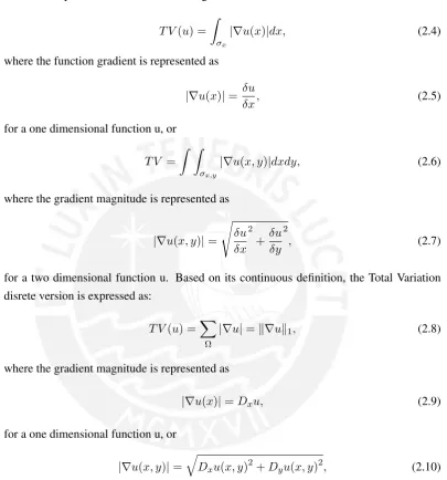
In [17], the use of Total Variation as a penalization criterion is introduced into regular-ization theory. The Total Variation of a signaluis defined as:

T V(u) =

Z

[image:13.595.124.530.149.584.2]

σx

|∇u(x)|dx, (2.4)

where the function gradient is represented as

|∇u(x)|= δu

δx, (2.5)

for a one dimensional function u, or

T V =

Z Z

σx,y

|∇u(x, y)|dxdy, (2.6)

where the gradient magnitude is represented as

|∇u(x, y)|=

s

δu δx

2

+ δu δy

2

, (2.7)

for a two dimensional function u. Based on its continuous definition, the Total Variation disrete version is expressed as:

T V(u) =X

Ω

|∇u|=k∇uk1, (2.8)

where the gradient magnitude is represented as

|∇u(x)|=Dxu, (2.9)

for a one dimensional function u, or

|∇u(x, y)|=

q

Dxu(x, y)2+Dyu(x, y)2, (2.10)

for a two dimensional function u. Dx andDy represent horizontal and vertical discrete

derivative operators, respectively.

Total Variation has a remarkable property which explains its versatility as part of the regularization term. The following Lemma [20] shows the main feature of such a constraint:

min

u T V(u) s.t. u(0) =a, u(1) =b, u:R→R, (2.11)

has as minimizer a monotonic in [a, b], not necessarily continuous function uˆ satisfying ˆ

u(0) = a,u(1) =ˆ bandT V(ˆu) = |b−a|. Figure 2.1 shows the possible solution subset for this problem and how oscillatory functions such as u5 may not be part of it. As the

(14)

0 0.1 0.2 0.3 0.4 0.5 0.6 0.7 0.8 0.9 0

0.2 0.4 0.6 0.8 1

u1

u4

u3

u5

u2

(a) (b)

Figure 2.1: Total Variation on one dimensional functions.

oscilatory nature,T V(u5)>|b−a|. Thus, it is not an element in the solution subset.

0.1 0.2 0.3 0.4 0.5 0.6 0.7 0.8 0.9 −10

−5 0 5 10 15 20 25 30

(a)α= 10−4

0.1 0.2 0.3 0.4 0.5 0.6 0.7 0.8 0.9 −10

−5 0 5 10 15 20 25 30

(b)α= 10−3

0.1 0.2 0.3 0.4 0.5 0.6 0.7 0.8 0.9 −10

−5 0 5 10 15 20 25 30

(c)α= 10−2

0.1 0.2 0.3 0.4 0.5 0.6 0.7 0.8 0.9 −10

−5 0 5 10 15 20 25 30

(d)α= 10−1

0.1 0.2 0.3 0.4 0.5 0.6 0.7 0.8 0.9 −10

−5 0 5 10 15 20 25 30

[image:14.595.128.526.406.532.2]

(e)α= 1

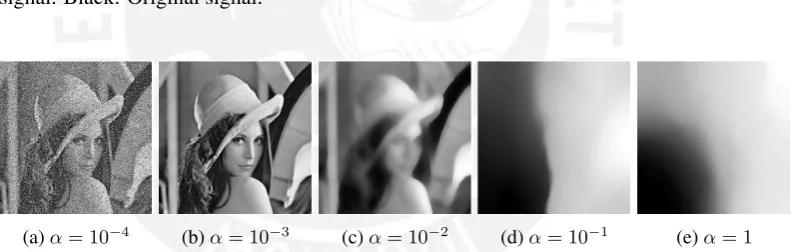
Figure 2.2: Regularization parameter impact for one dimensional functions. Red: Estimated signal. Black: Original signal.

(a)α= 10−4 _(b)α= 10−3 _(c)α= 10−2 _(d)α= 10−1 _(e)α= 1

Figure 2.3: Regularization parameter impact for two dimensional normalized functions (∈ [0,1]).

Equation (2.11) shows how the solution for the minimization problem does not favor a specific kind of function, whether smooth or edge-structured. Moreover, it rejects oscil-latory solutions while preserving edges. As a consequence, the Total Variation term is a favorable element for the image restoration problem which preserves features and adapts to a specific desired fitting level.

Following this concept, the Total Variation regularization cost function is described as:

min

u kKu−bk

m

m+λT V(u). (2.12)

(15)

The Total Variation regularization approach may be summarized in a phrase: ”Find a solution which approximates to the observation, but which has a minimum Total Variation”. It is shown that the cost function solution is unique and its existence can be proven under certain assumptions [17]. Solving this functional is a complex task since it is not differen-tiable [5, 6, 21]. Moreover, the regularization approach can also be seen as a scale selection based onλ, by which a certain level of detail preservation is defined. Figures 2.2 and 2.3 show the impact of the regularization parameter in the restoration of one dimensional and two dimensional signals, respectively.

Finally, given an observationB∈Rm×n×c, the Total Variation constraint is introduced by characterizing the solutionU∗ ∈Rm×n×cas:

u∗= arg min u 1 m

Ku−b

m m +λ n ∇u n n , (2.13)

where u∗,b are vectorized versions of the estimated image and the observation, respec-tively.∇urepresents the solution gradient magnitude, which can be modelled as its isotropic version(|∇u|=pP

n∈c(Dxun)2+ (Dyun)2)or its anisotropic version(|∇u|=|Dxu|+

|Dyu|). Forc ={1,2,3}we have thatu = [(u1)T(u2)T(u3)T]T is a 1D vector that

rep-resents a 2D color image. Both cost function terms consist on vector norms defined by (m, n∈R+).

The classic Total Variation formulation proposed on [17] focused on the Additive noise model scenario and consisted on anℓ2 _{data fidelity term and an}_ℓ1_{regularization term:}

u∗= arg min u 1 2

Ku−b

2 2 +λ ∇ u 1 . (2.14)

Although typically used on previous approaches, the fidelity term norm was kept since, for the statistics field, it was considered the best smooth edge-preserving cost function for such a noise model. On the other hand, several data fitting functions and their impact as fidelity terms have been studied in [22, 19]. It is shown that non-smooth data fidelity terms reach high quality minimizers for corrupted images characterized by containing non corrupted elements and outliers, which is the case of the Impulse noise model. The ℓ1 data fidelity term proofs to be more accurate for this scenario than theℓ2 term [14]. This approach is formulated as:

u∗= arg min u

Ku−b

1 +λ ∇u 1 . (2.15)

2.3 Risk Estimation

A common risk metric for defining the level of likeness between two signals based on the ℓ2_{norm is the Mean Squared Error (MSE) [5]:}

MSE(x,y) = 1 n

n−1 X

i=0

x(i)−y(i)2

(16)

wherex, y∈Rn. This tool is able to characterize the reconstructed image quality level, but only if the original image is available.

An alternative way for measuring the reconstruction quality level is by using an unbiased risk estimator, which does not require the original signal. Although the use of such metrics were originally confined to the White Gaussian noise case, its study and applications has been widely covered in the literature [8, 9].

2.3.1 Unbiased Predictive Risk Estimator

The Unbiased Predictive Risk Estimator (UPRE), also known as CL method [5], for the

Total Variation framework was proposed in [9]. As its original formulation, which was intended for the Tikhonov Regularization method, the UPRE estimates the MSE ofuλ for

b=Ku+η, whereη∼N(0, σ2). UPRET K is formulated as

UPRETK(λ) =

1 n||rλ||

2 2+

2σ2

n tr(ATK,λ

−σ2, (2.17)

rλ =Kuλ−b (2.18)

ATK,λ =K(KTK+λI)−1KT. (2.19)

whereuλrepresentsu∗for a specificλ. Given this risk estimation, it is possible to find the

optimalλvalue by searching in theλspace. Extending this concept to the Total Variation framework, UPRET V is denoted as

UPRETV(λ) =

1 n||rλ||

2₊2σ2

n tr ATV,λ

−σ2, (2.20)

ATV,λ=K(KTK+λL(uλ))−1KT, (2.21)

L(uλ) =DTxdiag Ψ′(uλ)Dx+DTydiag Ψ′(uλ)Dy. (2.22)

Since there is no linear operator than can describe the Total Variation solution, functionA, which depends onuλis introduced. The Total Variation regularization term is approximated

by

||u||TV=||ψ (Dxu)2+ (Dyu)2

||1, (2.23)

ψ(u) =pu+β2_, _(2.24)

whereψ(u)is a smooth approximation of the absolute value function which allows differ-entiation at the origin.

UPRETVinserts in the original formulation a parameter which depends onxλ. This

im-plies that a solutionxλmust be computed first, which increases the method’s computational

cost. Besides, [9] points out the high computational cost for computing Trace ATV,λ

(17)

estimation.

Let the Hutchinson trace estimator be defined as:

E(uTf(A)u)≃Trace(f(A)) (2.25)

whereuis a vector which entries are values 1 or -1 with 0.5 probabilities each. It has been proven that

1 N

N−1 X

n=0

(uT_nf(A)un)≃Trace(f(A)), (2.26)

whereN << M,A∈M×M. So, it is required to solve

uT_nf(A)un=uTnK KTK+λL(uλ)−1KTun. (2.27)

The proposed approach, in contrast with the original approach in [9], is to solve:

KT(K(r)) +λL(uλ)r=v (2.28)

forr, wherev=KT(u). Furthermore,L(uλ)rmay be represented as

D_xT(Ψ′(uλ)•Dx(r)) +DTy(Ψ′(uλ)•Dy(r)). (2.29)

So, this procedure requires a linear solver to estimate Trace(A).

2.3.2 Q Metric

In [23], The Q metric, a pseudo-local signal to noise ratio, is presented. Its formulation is based on the estimation of the gradient covariance matrix and its singular value de-composition. Based on this, the gradient’s dominant orientations and its energy charac-terizes each image patch in order to define its structure properties. This no-reference metric quantifies the image ”coherence measure”, allowing the analysis of the noise level in non-homoskedastic scenarios without depending on its model. It requires no prior knowledge about the noise variance.

The Q Metric is defined as:

Q=s1R, (2.30)

R= s1−s2 s1+s2

, (2.31)

G=U SVT =U s1 0 0 s2

!

v1

v2 !

, (2.32)

G=



  

px(1) py(1)

..

. ... px(n) py(n)



  

, (2.33)

(18)

the elements on a neighborhoodWn. Under this formulation,s1 represents the gradient’s

dominant orientation, whiles2 represents its perpendicular direction (s1 ≥s2≥0).

The metric requires consistent gradient components in the analyzed patches in order to obtain a good noise estimate. Thus, it is not capable of defining the noise level in homoge-neous regions. The basic idea behind this metric is the level of ”structure features” covered by each patch. So, for high noise levels, it is demonstrated that this metric is innacurate, mainly because the loss of structure.

2.4 Impulse Noise Set Estimation

For Mixed noise scenarios, the original Total Variation approach may suffer from bad re-sponses since it affects the entire image in the same way. Different approaches have been proposed in order to attack this issue, most of them based on the addition of terms to the cost function in order to fit the noise distributions. Figure 2.4 shows results from [1], a recent work based on the proposed method’s preliminary stages, and displays the reconstruction benefits of local vs. global restoration. A special case for this scenario is the Impulse over Gaussian Additive noise. Since the distortion introduced by it remains unchanged by the others, the corrupted pixel set may be easily identified.

In [2], this approach is used on the Salt and Pepper noise scenario by applying a local noise detector for finding the corrupted pixel set, and then treating them by applying a median filter. Then, the same concept is applied for a variational scheme by penalizing the corrupted pixel set only. Following this idea, a study on different Impulse noise detectors is presented.

2.4.1 Ranked Over Adaptive Median Filter

The Salt and Pepper noise detector based on an adaptive median filter applied in [2, Al-gorithm 1] is described. The noise pixel set of the observed image b withL channels is defined by:

N :{n∈C, l∈Ω : ˆbwln

n (l)6=bn(l)∧bn(l)∈ {vmin,vmax}}, (2.34)

whereˆbwln

n (l)is the output of the Ranked Over Based Adaptive Median Filter (RAMF) [24].

This filter analyzesK, a(2·w_nl + 1)×(2·wl_n+ 1)neighborhood centered atlin order to define whether this pixel is noise-corrupted or not. The neighborhood size is increased if the median of the neighborhood is equal to its minimum or maximun value, and the procedure is repeated until it reaches a maximum sizewmax. Then,lis defined as a noise-corrupted

pixel if it is equal to the maximum or minimum value in the neighborhood, in which case is replaced by the neighborhood median. In [2], manually selected values for wmax are

applied depending on the noise level.

The proposed algorithm defines the setW, which is zero if the elementlis noise-free and wl_n if it is noisy. This gives information about the local noise level for each noise-corrupted pixel. Moreover, the global noise levelp can be estimated asp˜= _N1 P

I[W6=0],

(19)

(a) Original image (b)90%noisy image

[image:19.595.129.525.70.489.2]

(c)90%Global regularization reconstruction (d)90%Local regularization reconstruction

Figure 2.4: Global versus local regularization approaches, as shown on the present work preliminary results [1].

2.4.2 Progressive Switching Median Filter

In [25], a progressive switching median filter (PSM) is proposed for treating images cor-rupted by Salt and Pepper noise. Its general framework is composed by an outlier detector for defining the noise pixel set, and a median filter for restoring it. Regarding the noise set estimation, the algorithm base its criteria in the median absolute difference (MAD). For this purpose, an iterative scheme is used, where an element is defined as corrupted if its observation is over a threshold.fi defines if the i-th element belongs to the noise set:

f_i(n)=







f_i(n−1) ,|u_i(n−1)−m(_in−1)|< Td

1 , else

where mi is the median value of a neighborhood centered at the i-th element. Initially,

(20)

iteration, the element intensities of the observation are modified in order to cope with the iterative scheme:

u(_in)=







m_i(n−1) ,f_i(n)6=f_i(n−1) u_i(n−1) ,f_i(n)=f_i(n−1)

After a number of iterations, the noise pixel set is defined byf_i(n). Tdis chosen based on

the noise level(p), which is based on an estimation with the same criteria:

p=

Pn−1

i=0 pˆi

n−1 (2.35)

ˆ pi =







0 ,|ui−mi|< T0

1 ,else

2.4.3 Impulse Weighting Function

In [26], an extension of the Bilateral filter introduced in [27] is proposed. A new weighting component is proposed based on the ROAD (Ranked-over Absolute Difference) statistic, which, in contrast with the Two-Stage methods, gives a continuous function of how much an element is ”Impulse-like” or not. This new component, which will be called Impulse Weighting Function (IWF) is defined as:

wI(x) =e

−ROAD₂_σ2(x)2

j _(2.36)

whereσj is a tunable parameter which defines the weighting penalization degree. By

applying a threshold to the function response, it is possible to classify the image elements into a two-stage scheme.

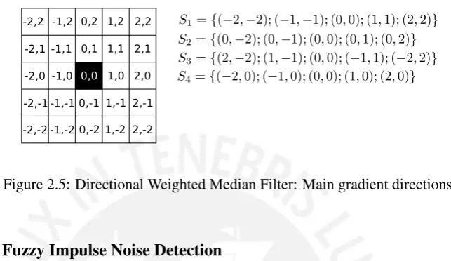
2.4.4 Directional Weighted Median Filter

A novel median filter intended for detecting Impulse noise was proposed in [28]. This directional weighted median filter (DWMF) features a weighting which depends on the intensity differences between local elements on four main directions. This design bases in the fact that a noise free image is characterized by locally smooth areas separated by edges. The difference on each direction shows if the smooth local region assumption is satisfied based on how big the variability on its main direction is. Following this, the intensity difference on each direction is defined as:

d(_i,jk)= X

(s,t)∈Sk

ws,t|yi+s,j+t−yi,j|, (2.37)

wherews,t describes a weighting function which gives more emphasis to the elements

(21)

ri,j =min{d(i,jk) : 1≤k≤4}. (2.38)

An Impulse noise element should be characterized by big differences in all four direc-tions due to its outlier nature, while edge elements and elements in flat regions should at least have one small difference. Thus, largeri,j values correspond to outliers. Figure 2.5

shows the four main directions.

-2,2 -1,2 2,2 1,2 2,2

-2,1 -1,1 2,1 1,1 2,1

-2,2 -1,2 2,2 1,2 2,2

-2,-1 -1,-1 2,-1 1,-1 2,-1

[image:21.595.162.484.178.364.2]

-2,-2 -1,-2 2,-2 1,-2 2,-2

Figure 2.5: Directional Weighted Median Filter: Main gradient directions.

2.4.5 Fuzzy Impulse Noise Detection

In [29], the Fuzzy Impulse noise Detection and Reduction Method (FIDRM) is introduced. Its noise estimation stage is a fuzzy-ruled system established based in the GOA filter [30]. Fuzzy gradient values for an element are defined by applying a membership degree function to the element finite difference based gradients, which are taken between the element and its eight neighbors.

∆c,dI(a, b) =I(a+c, b+d)−I(a, b); (a, b, c, d)∈ {−1,0,1} (2.39)

Each pixel features eight basic gradients, each with two related gradients associated, which are its two finite difference gradient neighbors in the same direction. Figure 2.6 shows the eight basic gradient and their related gradients, as well as the main directions. Fuzzy rules for identifying Impulse noise pixels are based on membership functions for the gradients magnitude and sign. Algorithm 1 shows the applied fuzzy rules.

-2,2 -1,2 2,2 1,2 2,2

-2,1 -1,1 2,1 1,1 2,1

-2,2 -1,2 2,2 1,2 2,2

-2,-1 -1,-1 2,-1 1,-1 2,-1

-2,-2 -1,-2 2,-2 1,-2 2,-2

Figure 2.6: Fuzzy Impulse noise detection: Basic and Related gradients.

[image:21.595.175.473.588.681.2]

(22)

Algorithm 1Fuzzy Impulse noise detection

initialization;

if ∆basicI(i, j)is largeand∆related 1I(i, j)is small

or ∆basicI(i, j)is largeand∆related 2I(i, j)is small

or ∆basicI(i, j)is big positiveand∆related 1I(i, j)is big negativeand∆related 2I(i, j)is big negative

or _∆_basic_I₍_{i, j}₎_{is big negative}and_∆_{related 1}_I₍_{i, j}₎_{is big positive}and_∆_{related 2}_I₍_{i, j}₎_{is big positive}

then

∆(F)I(i, j)is large

end

if most of the∆(F)

I(i, j)are large

then

I(i, j)is an Impulse noise pixel

end

2.5 Gaussian Additive Noise Variance Estimation

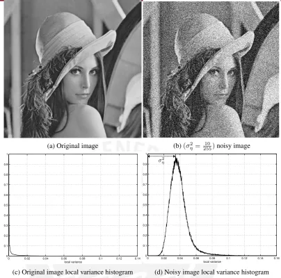
In [31], a noise variance estimator with a very simple concept and interesting results, which bases on the low variability areas natural images contains, is presented. For the Gaussian Additive noise scenario, the estimator is based on the variances from multiple patches from the entire image. Based on this variance collection, it is proposed to use its mode as an unbiased estimator.

The variance estimation is crucial for the multiple noise scenarios, including the Gaus-sian Additive scenario, since most of the filtering processes requires the image noise level [5]. Based on an Additive noise scenario:

b(x, y) =u(x, y) +η(x, y), (2.40)

wherebis the degraded image (observation),uis the original image, andηis the additive noise, the overall variance can be expressed as:

σ_b2₍_x,y₎=σ_u2₍_x,y₎+σ_η2 (2.41)

Whereσ_b2₍_x,y₎,σ2_u₍_x,y₎ are local variances. So, ifσ2_u₍_x,y₎ = 0(homogenous local region), thenσ2

b(x,y) =σ2η. In order to exploit this condition to find the noise level, an homogenous

zone selection is required. Assuming an ideal case: σ2_η =σ_min2 =minx,y{σ2_b₍_x,y₎}.

How-ever, in a real scenario, this estimator is sensitive to outliers. Another common employed estimator isσ2

MAD= 1.4826·MAD(yijH), which is the median absolute deviation of the

high-est wavelet decomposition stage of a signal, i.e. MAD(f) = median(f −median(f)). Beside the mentioned methods, A wide variety of them is covered in [24].

The effect of adding White Gaussian noise in the sample variances along patches in the image corresponds to a right shift in its distribution, i.e. in its histogram. This reflects in a uniform increase in the observation variance itself. The literature suggests based in this phenomenom that an effective noise estimator based on the population distribution of the variance is the mode. Modeling the noise as a Gaussian distribution and assuming a constant image scenario, it is shown that if we choose

σ_η2 = 1 N

X

(23)

(a) Original image (b)(σ2

η =

10

255)noisy image

0 0.02 0.04 0.06 0.08 0.1 0.12 0.14

0 0.1 0.2 0.3 0.4 0.5 0.6 0.7 0.8 0.9 1

local variance

(c) Original image local variance histogram

0 0.02 0.04 0.06 0.08 0.1 0.12 0.14 0.16 0

0.1 0.2 0.3 0.4 0.5 0.6 0.7 0.8 0.9 1

local variance

[image:23.595.122.527.71.471.2]

(d) Noisy image local variance histogram

Figure 2.7: Gaussian Additive noise estimation by local variance histogram approach.

we obtain the maximum likelihood estimator for σ2_sample. Another estimator which gets close toσ_η2for N large isM ode{σ2

sample}.

M ode{σ_sample2 }=σ2N−3

N−1, (2.43)

N−1

N−3M ode{σ

2

sample}=σ2, (2.44)

For typical natural images, which mostly contains homogenous zones, the variance dis-tribution has its peak around0. Analyzing the distributions of a test picture set and approxi-mating them to known statistical models, it is shown that, depending on the variability ratio between image and noise, the mode is not the actual Maximum likelihoodσ2

η estimation,

(24)

Proposed Restoration Framework

Given the previous concepts, aℓ1 _plus_ℓ2 _{Total Variation formulation capable of restoring}

images under Impulse over Gaussian Additive noise is introduced, and an optimal regular-ization parameter estimation framework is proposed. Additionally, the framework focuses also on the Impulse noise scenario as a particular case of the Impulse over Gaussian Ad-ditive case. Regarding the Gaussian AdAd-ditive noise scenario, since the proposed frame-work includes the UPRE, which remarkable performance for the Gaussian Additive noise scenario has already been covered in the literature (refer to [17, 4] for more details), the proposed framework does not focus on this noise model.

For a non-mixed noise model like the Gaussian Additive or Impulse scenario, there are several methods that successfully estimate the corrupted pixel set and noise level such as those mentioned in Section 2. However, none of this methods covers the scenario where more than a single noise model is present. Furthermore, the classic Total Variation cost function parameters are selected focusing on single noise models. Finally, a well condi-tioned metric is required in order to define an optimal regularization parameter. In the following, this requirements are analyzed in detail in order to propose a method that en-compasses them. Also, the framework proposed in [1, 4] is revisited in order to extend such concepts to a general denoising procedure.

3.1 Salt and Pepper Noise Scenario Approach: Spatially

Adap-tive IteraAdap-tively Reweighted Norm

An image restoration method for the Salt and Pepper noise model is stated in the prelimi-nary work published in [1], which uses a modification on theℓ1 TV functional. By taking advantage of theℓ1TV functional benefits for this noise model shown in [14, 19], the pro-posed approach consists on applying a local fashionedℓ1_{TV regularization on an estimated}

noise set obtained by a two-phase filter. The following section describes its framework.

3.1.1 Iteratively Reweighted Norm Algorithm

The Iteratively Reweighted Norm (IRN) algorithm [21, 32] is a computationally efficient and flexible Total Variation minimization method for grayscale and color images that can

(25)

handle thep >0andq≤2norms in the regularization and fidelity terms, respectively. This includes the ℓ2-TV andℓ1-TV as special cases. The algorithm attacks the minimization problem basing on the Iteratively Reweighted Least Squares (IRLS) approach [33], i.e. by representing the ℓp _and_ℓq _{norms by their equivalent weighted}_ℓ2 _{norms in an iterative}

fashion. Given the IRLS method, the cost function

1 r||u||

r r=

1 r

X

i

|ui|r, (3.1)

can be iteratively approaximated by

1 2||W

1/2_u_||2 2 =

1 2u

T_W_u₌ 1

2

X

i

wiu2i, (3.2)

where

W = 2

r diag(|u|

r−2_), _(3.3)

which is estimated iteratively by using the cost function minimizer from the previous itera-tion (u).

Following this, the IRN approach, which converges to the solution of (2.13), is ex-pressed as:

min

u T

(k)₍_u_{) =} 1

2

W_F(k)1/2(u−b)

2

+λ 2

W_R(k)1/2Du

2

, (3.4)

where

W_F(k) = diagτF,ǫF(u

(k)₋_b₎_, _(3.5)

W_R(k)=I2L⊗Ω(k), (3.6)

Ω(k)= diag τR,ǫR

X

n∈C

(Dxu(nk))2+ (Dyu(nk))2

!!

, (3.7)

τF,ǫF(x) =

(

|x|p−2 _if_|x|_{> ǫ}

F

ǫp_F−2 if|x| ≤ǫF

, (3.8)

τR,ǫR(x) =

(

|x|(q−2)/2 _if_|x|_{> ǫ}

R

0 if|x| ≤ǫR

, (3.9)

D=IL⊗[DxTDyT]T, (3.10)

ILis anL×Lidentity matrix,⊗is the Kronecker product, andLis a scalar which depends

(26)

to avoid numerical problems whenu(k)−bor X

n∈C

(Dxu(nk))2+ (Dyu(nk))2has zero-valued

components.

3.1.2 Local Regularization

A Total Variation cost function modification is proposed. This new cost function of interest is the modifiedℓ1-TV problem:

min

u T(u) =

Λ−1(u−b)

1

+

s X

n∈C

(Dxun)2+ (Dyun)2

1

, (3.11)

It is straighforward to check that ifΛis fixed, the IRN algorithm can be used to solve (3.11). The equivalent weightedℓ2version of the modifiedℓ1-TV problem can be written as:

min

u T

(k)₍_u_{) =} 1

2

W_F(k)1/2Λ(k)−1/2(u−b)

2

+1 2

W_R(k)1/2Du

2

, (3.12)

where Λ(k) _> ₀_{is a diagonal matrix defined in some fashion. Since (3.12) is quadratic}

and its Hessian ∇2T(k)(u) = W_F(k)Λ(k)−1+DTW_R(k)Dis greater than zero, then the minimum of (2.13) can be reached by iteratively solving

W_F(k)Λ(k)−1+DTW_R(k)Du=W_F(k)Λ(k)−1b. (3.13)

By replacing a scalar parameter by a vector, it is shown that the new Total Variation solution is capable of penalizing each pixel in a particular way [1]. Given this new feature, the way Total Variation fits to noise models acquires more flexibility, and thus allows better reconstruction results for more complex noise models. By approximating this new cost function toℓ2norms by applying the Iteratively Reweighted Norm algorithm, the result is a Spatially Adaptive IRN algorithm (SAIRN). Algorithm 2 presents the resulting method.

3.1.3 Salt and Pepper Noise Estimation

The Salt and Pepper noise detector based on the adaptive median filter described in (2.4.1) is used for the outliers detection. The proposed algorithm defines the setW, which is zero if the elementlis noise-free andwl

nif it is noisy. This gives information about the local noise

level for each noise-corrupted pixel. Note that the global noise levelpcan be estimated as ˜

p= _N1 P

I[W6=0], whereN is the number of pixels andI is the indicator function.

3.1.4 Parameter Update

(27)

Algorithm 2Spatially Adaptive IRN algorithm forℓ1-TV Initialize

Estimate setW fromb Λ(0)_{= diag(}_I

[wl

n(l)>0]) + 10

−6_diag(_I [wl

n(l)==0]) u(0,0)= I+ Λ(0)DTD−1

b

form= 0,1, ..,M

for k= 1,2, ..,K

W_F(k) = diag τF,ǫF(u

(m,k−1)₋_b₎

forp= 1 Ω(_Rk) = diag τR,ǫR (Dxu

(m,k−1)₎2_{+ (D}

yu(m,k−1))2

forq= 1

W_R(k) = Ω

(k)

R 0

0 Ω(_Rk)

!

u(m,k)=

I+ Λ(m)W_F(k)−1DTW_R(k)D

b

end

r =u(m,K)−b

estimate pˆ (via (3.14)) compute Λ(m+1) (via (3.15))

endm= 0,1, ...

The local noise estimator is defined as:

ˆ pn(l) =

1 M

X

k∈K_wln(l)

|rn(l)| (3.14)

whereM = (2·wl

n+ 1)2andKwl

n(l)is defined as in (2.4.1). The spatially dependant regu-larization parameterΛis initialized asΛ(0)= diag(λ(0)₎_{, with}_λ(0)_{(l) = diag(}_I_[_wl

n(l)>0]) + 10−6_diag(_I

[wl

n(l)==0]). After solving (3.11),pˆn(l)is computed in order to obtain the regu-larization parameter updatesλ(nm)(l)in a spatially dependant fashion:

λ(_nm)(l) =







ρ−1·λ(nm−1)(l) ifpˆn(l)<p˜·σ

ρ·λ(nm−1)(l) ifpˆn(l)>p˜·σ

, (3.15)

whereρ, σare constant values andp˜is the estimated global noise level.

The SAIRN focuses on the Salt and Pepper noise scenario. As an initial step, it uses the RAMF as an Impulse noise detector. Following this, an initial (Λ(0)) is defined to start the IRN iterations. at each step, (Λ(k)_{) is updated according the remaining noise in}

(r=|b−u(k)|).

3.1.5 Regularization Parameter Selection without Update Strategy

(28)

local approach it uses can be modeled as a variational method generalization for low noise level cases, since it is capable of restricting its penalization areas based on the estimated noise set without neglecting the noise free elements. Consequently, a new adaptive scheme was proposed as a preliminary stage for this work with a considerable change in the update criteria, which has proven to get a faster convergence rate [4].

For the ℓ1 TV image denoising under Impulse noise scenario, the elementwise Total Variation solution for a particular (λ) is given by the following:

u(i,j,λ=0)=b(i) (3.16)

u(i,j,λ→∞)=

u(i+1,j)+u(i,j+1)

2 , (3.17)

for a forward operator based finite differentiation and the anisotropic Total Variation model. Hence, local solutions lie between the observation pixel value (b(i,j)) and a pixel-based

average which bases on its neighborhood intensity values (u(i+1,j)+u(i,j+1)

2 ).

Following the arguments stated in [31], the information of a natural image is contained in its edges and form coherent structures of homogeneous regions. This means that most of the noise pixels, except the ones located close to edges and other features, have an original intensity which is very close to its neighborhood. On the other hand, as mentioned in Section 2, Impulse noise pixels holds no information about their real intensity.

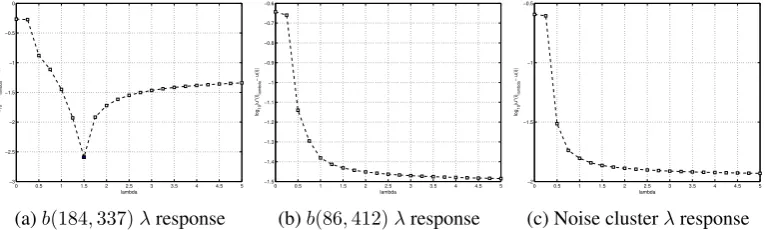
Figure 3.1 shows noise pixels for three different image regions on the (s = 0.05) Im-pulse corrupted (gray) Lena: An edge region, a flat region, and a noise cluster region. In ad-dition, Figure 3.2 presents theλimpact for such structures, based on the absolute difference between the original and reconstructed intensities. Theλsearch shows how the edge region reaches an accurate reconstruction inside the range defined by b(i,j) and

u(i+1,j)+u(i,j+1)

2 .

On the other hand, the flat region and the noise cluster reach good estimates which tend to

u(i+1,j)+u(i,j+1)

2 . This behavior is coherent with the previous argument for flat regions. For

the edge region and noise cluster, the optimal λ may depend on how big is the intensity range defined by[b₍_i,j₎;u(i+1,j)+u(i,j+1)

2 ].

Based on this, it is proposed to minimize the Total Variation fidelity term impact on the noise pixel set, which reflects in aΛ with big valued elements. This forces a noise pixel set solution based purely on their neighbors values. This implies no loss of certainty, since Impulse noise pixels holds no original information. On the other hand, sinceΛ penalizes only the noise pixel set, the Total Variation regularization term for the noise free pixels is minimized, so they remain unaltered. This argument can also be applied to the isotropic representation of the Total Variation term, since it also depends on its neighbors.

Finally, the optimal Total Variation solution is defined by solving the IRN scheme:

W_F(k)Λ(k)−1+DTW_R(k)Du=W_F(k)Λ(k)−1b. (3.18)

for u. the SAIRN defines Λasdiag(_λ1

0, ...,

1

λn−1

(29)

λi =







0 ,i /∈ N

[image:29.595.128.528.207.560.2]

c >>1 ,i∈ N (3.19)

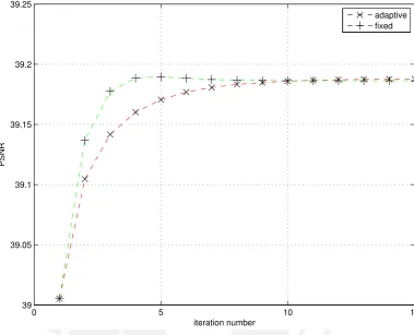
Figure 3.3 shows the reconstruction quality (PSNR) contrast between the adaptive λ iterative scheme, withρ= 0.75andσ = 0.5, and the fixedλiterative scheme for grayscale Lena under the Impulse noise scenario(s= 0.25). Convergence for the fixed scheme con-siderably increases, while the quality remains almost the same without the need of updating Λ.

0 100 200 300 400 500

50

100

150

200

250

300

350

400

450

500

(a) Impulse noise corrupted (gray) Lena

330 335 340 345

178

180

182

184

186

188

190

(b) Impulse noiseb(184,337)on an edge region

404 406 408 410 412 414 416 418 420

80

82

84

86

88

90

92

(c) Impulse noiseb(86,412)on an flat region

455 460 465 470

332

334

336

338

340

342

344

[image:29.595.131.514.608.723.2]

(d) Impulse noise cluster region

Figure 3.1: Image structure regions for the Impulse noise scenario.

0 0.5 1 1.5 2 2.5 3 3.5 4 4.5 5 −3

−2.5 −2 −1.5 −1 −0.5 0

log

10

|u*(i)

lambda

− u(i)|

lambda

(a)b(184,337)λresponse

0 0.5 1 1.5 2 2.5 3 3.5 4 4.5 5 −1.5

−1.4 −1.3 −1.2 −1.1 −1 −0.9 −0.8 −0.7 −0.6

log

10

|u*(i)

lambda

− u(i)|

lambda

(b)b(86,412)λresponse

0 0.5 1 1.5 2 2.5 3 3.5 4 4.5 5 −2

−1.5 −1 −0.5

log

10

|u*(i)

lambda

− u(i)|

lambda

(c) Noise clusterλresponse

(30)

0 5 10 15 39

39.05 39.1 39.15 39.2 39.25

iteration number

PSNR

[image:30.595.133.513.76.383.2]

adaptive fixed

Figure 3.3: Iterative fixed approach versus Iterative adaptive scheme (with ρ = 0.65 and σ = 0.5) quality contrast for (gray) Lena under the Impulse noise scenario (s= 0.25).

3.2 Impulse over Gaussian Additive Noise Scenario Approach:

Modified Spatially Adaptive Iteratively Reweighted Norm

The SAIRN achieves high quality results for the Salt and Pepper noise scenario because, with high probability, the ℓ1 Total Variation solution derives from noise free image ele-ments. For relatively low noise corruption levels, most of the Impulse noise corrupted elements’ neighborhood belongs to noise free elements. Under these circumstances, The use of either statistical filters or variational methods, such as the RAMF andℓ1Total Varia-tion respectively, have proven to give good results [5]. For relatively high noise corrupVaria-tion levels, corrupted pixel clusters appears. In contrast to the former case, filtering under this conditions attains poor quality results since the output for each element depends on its cor-rupted neighbors. Given this scenario, SAIRN iterative approach leads to a progressive cluster shrinkage. Due to the fact that some of the elements within a cluster, those in the cluster edges, have uncorrupted elements within their neighborhood, theℓ1 Total Variation output they attain is based on trusty information, and so it can be seen as an accurate inter-polation. Then, the iterative behavior can be seen as a chain interpolation: a set of corrupted elements within a cluster finds a stable solution at each iteration, giving accurate informa-tion to the rest of elements within the cluster. This scheme is kept until the entire cluster finds an unfluctuating solution.

(31)

un-able to attain high quality outputs because the entire image is distorted. Any attempt of reconstructing the Impulse noise pixels based on whether filtering or variational methods derives from corrupted elements. Furthermore, the SAIRN algorithm targets only the Im-pulse noise, leaving the Gaussian Additive noise behind. Based on this limitations, a novel iterative scheme is proposed based on the SAIRN procedure. However, consistent modifi-cations are done in order to surpass this new scenario.

Aℓ1_plus_ℓ2_{locally regularized Total Variation reconstruction is proposed for this Mixed}

noise model. This means two separate reconstructions: aℓ1 TV reconstruction for the Im-pulse noise pixel set and aℓ2 TV reconstruction for the Gaussian Additive noise pixel set. In addition to the already stated SAIRN framework, a noise set estimation which discrimi-nates between both models and an accurate criteria for choosing the optimal regularization parameter for the ℓ2 TV reconstruction is required. Furthermore, since both separate re-constructions derives directly from corrupted pixels, a decision must be made in order to choose which noise model must be dealt with first.

3.2.1 Impulse Noise: Outliers Detection

For this Mixed noise scenario, it is still possible to recognize the Impulse corrupted pixel set N, since they are still represented as outliers. Of course, this also implies the identification of the Additive corrupted pixel set. However, experimental results show that the RAMF accuracy descreases considerably, specially under high Gaussian Additive noise level. The proposed scheme uses two different observations in order to obtain a more accurate estima-tion ofN. The DWMF and the RAMF observations are combined in order define estimate the corrupted set. So, letNDWMFdenote the element set defined as Noise by the DWMF,

i.e.

min{d(_i,jk)}> Td: 1≤k≤4, (3.20)

AndN the element set defined as noise by the RAMF, i.e.

NRAMF:{n∈C, l∈Ω : ˆbw

l n

n (l)6=bn(l)∧bn(l)∈ {vmin, vmax}}, (3.21)

Then, the estimated Impulse noise set is defined as

N :NRAMF∩ NDWMF (3.22)

Following this, the Gaussian Additive noise corrupted set can be defined as

G : Ω\ N (3.23)

3.2.2 Gaussian Additive Noise: Local Risk Estimation

(32)

It is proposed to find a solution for the Impulse corrupted element set based onNRAMF∩

NDWMFas an initial step. Since, ideally, only the Impulse noise corrupted pixels are

modi-fied, the Gaussian Additive noise elements suffer no information loss.

After this step, the resulting image is formed by the Gaussian Additive noise pixels and their interpolation which replaces the Impulse noise pixels. This new image cannot be taken as a plain Gaussian Additive noise scenario, even when no outliers remain, for two main reasons: First, the interpolation does not holds any information about the original Impulse noise pixels. Second, applying this scheme may modify the noise properties due to the fact that new intensities in different proportions are being introduced to the new image. That is, if there was an initial Additive noise distribution affecting the original image, then the resulting image does not hold it.

The purpose of creating this intermediate output is to find an Additive corrupted element set Total Variation solution based on coherent non-outlier intensities. This is similar to the plain Impulse noise case, where the Impulse pixel set find new intensities based noise free elements only. However, in this new scenario, the only pixels holding true information are the Additive noise elements. So, an iterative procedure first regularizes N based on the Additive noise elements in order obtain structure-coherent intensities, and then regularizes Gbased on this new intensities.

By using the UPRE, an accurateℓ2_{TV reconstruction for the Gaussian Additive noise}

scenario may be achieved by searching for the optimal regularization parameter as the risk minimizer in theλspace [9]. However, under a Mixed noise scenario, the UPRE method needs to be modified as a local operator so that it performs over a specific pixel set and not the entire image. In the following, we introduce a UPRE modification in order to apply it in a local fashion.

Let MSE(g) = MSE(u(_λg)) denote the mean square error of the estimated Gaussian corrupted elements set. This risk measurement tells the error between the original and the restored elements in G by a specific λ. In order to estimate the risk measurement, i.e. the UPRE for this set, then it must only take into account the elements in G. Let Wg =diag(w0, ..., wn−1), where

wi=







0 ,i /∈ G 1 ,i∈ G

then, using this mask into the UPRE calculation:

UPRE(g)= kWgrλk |G| +

ˆ σ2

η

|G|Trace(WgA(uλ))−σˆ

2

η (3.24)

An important detail is that, since the UPRE is applied to a portion of the image, thenˆσ2

should take into account just the elements belonging toG. This is accomplished by taking into account only the very same elements when estimating the noise variance.

(33)

modifi-cation is reflected as:

r=vTWg(K(KTK+λL(uλ))−1KT)v (3.25)

or

r=vT₀(KTK+λL(uλ))−1v1 (3.26)

where v0 = KTWgv and v1 = KTv. So, the requirement of a solver for (KTK +

λL(uλ))r=v1is kept.

Given this modification, a Golden search on theλspace is proposed to find the UPRE minimizer and estimate the optimal regularization parameter for the localℓ2TV reconstruc-tion.

3.2.3 Modified Spatially Adaptive Iteratively Reweighted Norm

(34)

Algorithm 3 Modified Spatially Adaptive Iteratively Reweighted Norm for the Impulse over Gaussian Additive noise scenario

Initialize

EstimateN : NRAMF∩ NDWMFfromb

EstimateG: Ω\ N fromb

Λi =λ0diag(I[i∈N]) +ǫdiag(I[i /∈N]), λ0 >>1, ǫ∈R+<<1

u(0) = I+ ΛiDTD−1b

// Solve local _ℓ1 TV for b

fork= 1,2, ..,K

W_F(k)= diag τF,ǫF(u

(k−1)₋_b₎

forp= 1 Ω(_Rk)= diag τR,ǫR (Dxu

(k−1)₎2_{+ (D}

yu(k−1))2forq= 1

W_R(k)= Ω

(k)

R 0

0 Ω(_Rk)

!

u(k)=

I+ ΛiW_F(k)

−1

DT_W(k) R D

b

end

Calculateλ∗=arg min_λUPRE(_{T V,λ}g) (u(K)) Λg=λ∗diag(I[i∈G]) +ǫdiag(I[i /∈G])

v(0) = I+ ΛgDTD−1u(K)

// Solve local _ℓ2 TV for u

form= 1,2, ..,M

W_F(m)= diag τF,ǫF(v

(m−1)₋_u(K₎ )

forp= 2 Ω(_Rm)= diag τR,ǫR (Dxv

(m−1)₎2_{+ (D}

yv(m−1))2forq = 1

W_R(m)= Ω

(m)

R 0

0 Ω(_Rm)

!

v(m)=

I+ ΛgW_F(m)

−1

DT_W(m) R D

u(K)

end

w(0) = I+ ΛiDTD−1v(M)

// Solve local _ℓ1 TV for _w

fork= 1,2, ..,K

W_F(k)= diag τF,ǫF(w

(k−1)₋_v(M₎ )

forp= 1 Ω(_Rk)= diag τR,ǫR (Dxw

(k−1)₎2_{+ (D}

yw(k−1))2forq = 1

W_R(k)= Ω

(k)

R 0

0 Ω(_Rk)

!

w(k)=

I+ ΛiW_F(k)

−1

DTW_R(k)D

v(M₎

(35)

Experimental Results

The proposed framework is evaluated under Impulse noise and Impulse over Gaussian Ad-ditive noise, as depicted in Section 3. A contrast between the present work and the results reported on [2, 21, 32] and [35, 3, 4] is elaborated in order to show its performance against the state of the art algorithms. Each algorithm in the proposed framework is evaluated under different noise conditions against the state of the art algorithms. Furthermore, an evalua-tion on the SAIRN update scheme parameters (ρ;σ) reconstruction quality impact for the Impulse noise scenario is included. The evaluated quality metrics are the following:

SNR 10 log₁₀ Nσ

2_{_u∗_}

ku−u∗_k2 2

,

PSNR 10 log₁₀N(max{u})

2

ku−u∗k2 2

,

and SSIM [36], whereN is the number of pixels in all the image layers. The simulations are carried out using Matlab code on a 3GHz. Intel core i7 processor (1024KB. L2 Cache, 4GB. RAM).

4.1 Spatially Adaptive Iteratively Reweighted Norm: Update

Scheme Parameters Evaluation

The output for different SAIRN update parameter values (ρ; σ) is presented in order to show their reconstruction quality impact. Figures (4.11 - 4.13) show the quality results for (gray) Lena, (gray) Peppers and (gray) Bridge; fors={5%; 25%; 75%},σin the range of [0.25−1.25] (steps of0.5) andρin the range of [0.6−5.0].

Regardingρ, while the curves does not show an optimal value, ρ = 0.6 andρ = 0.7 show the best reconstruction quality for (gray) Lena and (gray) Peppers in most sandρ scenarios. On the other hand, covered σ values show no considerable impact for s = {25%; 75%} on the image test set. However, fors = 5%, ρ = 1.25 shows a slight re-construction quality increase for (gray) Lena and (gray) Bridge, while a slight decrease for (gray) Peppers. Finally, results also show how ρ > 1 has an unfavorable impact in the reconstruction quality, which keep the same reconstruction quality along all the iterations.

(36)

ˆ σ2

η

MSEgrid UPREgrid,tr. comp. UPREgrid,tr. est. UPREgolden,tr. est.

642px. 1282px. 642px. 1282px. 642px. 1282px. 642px. 1282px.

10

255 0.01 0.01 0.01 0.01 0.01 0.01 0.0121 0.0122

20

255 0.025 0.025 0.03 0.025 0.03 0.03 0.0243 0.0319

30

255 0.045 0.04 0.045 0.04 0.045 0.05 0.0441 0.0441

40

255 0.06 0.06 0.07 0.06 0.07 0.075 0.0592 0.0714

50

255 0.075 0.08 0.08 0.08 0.075 0.09 0.0789 0.0911

Table 4.1: UPRETV accuracy: λ∗ for the computation and estimation of Trace(ATV).

computa-tion; UPREgrid, tr.est.: UPRE grid search by Trace(ATV)estimation; UPREgolden, tr.est.: UPRE

golden Search by Trace(ATV)estimation.

Although the proposed framework does not include the SAIRN iterative (Λ) update scheme, the evaluation shows how, under different scenarios, there may not be optimalρ andσvalues. Instead, for images with different features and structural characteristics, such parameters may be specifically selected in order to obtain the best outcome.

4.2 Gaussian Additive Noise Risk Estimation Performance

UPRE computation implies a great cost since it depends upon the Trace(ATV)computation.

ATVconsiderably increases its dimensions for a relatively big observation, which means a

serious obstacle. As mentioned in Section 3, the present work uses an alternative approach which does not calculate Trace(ATV). Instead, it uses the Hutchinson Trace Estimator [9],

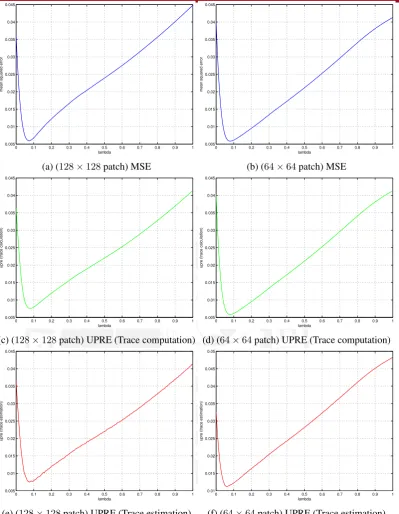
which dramatically reduces the computational requirements. On the other hand, the pro-posed method estimates λ∗ as the UPRE minimizer by searching in the λ space, which requires theℓ2 TV calculation for severalλvalues. Following this, an evaluation of both methods, UPRE computation vs. Hutchinson estimation, for the White Gaussian Noise sce-nario is presented. Additionally, a Grid search and a Golden search for the λ∗ estimation is applied. The accuracy of both methods regarding the Trace(ATV) is analyzed on two

patches of (64 x 64) and (128 x 128) pixels on (gray) Lena corrupted by White Gaussian noise withσ2

ηin the range of [25510 −25550 ] (steps of25510). Table 4.1 presents the achievedλ∗

for each case. Since the test does not include processing time, it is important to remark that the Trace(ATV)calculation time is around fifteen times the time required by the Hutchinson

(37)

ˆ σ2

η

MSEgrid UPREgrid,tr. comp. UPREgrid,tr. est. UPREgolden,tr. est.

642px. 1282px. 642px. 1282px. 642px. 1282px. 642px. 1282px.

10

255 0.01 0.01 0.015 0.01 0.015 0.01 0.0047 0.0122

20

255 0.02 0.025 0.02 0.025 0.02 0.025 0.0244 0.0244

30

255 0.035 0.03 0.025 0.03 0.025 0.03 0.0319 0.0441

40

255 0.05 0.05 0.04 0.05 0.04 0.05 0.0441 0.0592

50

255 0.065 0.07 0.045 0.075 0.045 0.06 0.0714 0.0811

Table 4.2: Local UPRETVaccuracy: λ∗for the computation and estimation of Trace(ATV).

computa-tion; UPREgrid, tr.est.: UPRE grid search by Trace(ATV)estimation; UPREgolden, tr.est.: UPRE

golden Search by Trace(ATV)estimation.

4.3 Gaussian Additive Noise Variance Estimation Performance

A contrast between the ground truth σ_η2 for the Gaussian Additive noise corrupted pixels, i.e. the elements which belong toG, and the local variance estimator introduced in Section 3 is elaborated in order to analyze its accuracy. The ground truth variance is defined as σ2_η,sample= _|G|1 P

Gu(i)−µ(u), whereµ(u)is the sample mean. The test is performed on

(gray) Lena, with Gaussian Additive noise withσ2

η = [25525 − 25575](steps of 25510), and Salt

and Pepper noise withs= [0.25−0.75](steps of0.25). Figure 4.2 shows the test results. It is important to remark that the Additive noise is applied to the entire image, so after the Impulse noise corruption, the Additive noise corrupted element setGnot necessarily holds the originalσ2_η. The results show thatσˆ_η2gets significantly closeσ_η2in most cases.

4.4 Impulse Noise Outliers Detection Performance

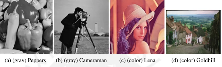
The SAIRN proposed method makes use of the RAMF for outliers detection, which are considered noise corrupted elements under the Salt and Pepper noise scenario. In contrast, the present framework requires an accurate Impulse noise estimation whether on a Mixed noise scenario or in a plain Impulse noise scenario. For this purpose, several Impulse noise estimation methods are evaluated. The methods are: RAMF, PSM, IWF, DWMF, FIDRM Detector, MAD, and a Modification of the CWMF proposed in [4]. This methods, all of them based on two-stage ranked order filters and introduced in Section 2, are tested on a Salt and Pepper over Gaussian Additive noise scenario for a test image set formed by grayscale (Peppers, Cameraman) and color (Goldhill, Lena) images. Figure 4.3 show the image set. For the evaluation, ση varies within [₂₅₅5 − ₂₅₅15] (steps of ₂₅₅5 ) and s within

[30%−90%] (steps of 0.3). Each test consists of fifteen iterations. Each performance is measured by the ratio of True positives vs. the ground truth noise set, False positives vs. the number of pixels in the image, and the required time for each method. Figures (4.14 - 4.21) show the performance results.

(38)

Cam-0 0.1 0.2 0.3 0.4 0.5 0.6 0.7 0.8 0.9 1 0.005

0.01 0.015 0.02 0.025 0.03 0.035 0.04 0.045

lambda

mean squared error

(a) (128×128patch) MSE

0 0.1 0.2 0.3 0.4 0.5 0.6 0.7 0.8 0.9 1

0.005 0.01 0.015 0.02 0.025 0.03 0.035 0.04 0.045

lambda

mean squared error

(b) (64×64patch) MSE

0 0.1 0.2 0.3 0.4 0.5 0.6 0.7 0.8 0.9 1

0.005 0.01 0.015 0.02 0.025 0.03 0.035 0.04 0.045

lambda

upre (trace calculation)

(c) (128×128patch) UPRE (Trace computation)

0 0.1 0.2 0.3 0.4 0.5 0.6 0.7 0.8 0.9 1

0.005 0.01 0.015 0.02 0.025 0.03 0.035 0.04 0.045

lambda

upre (trace calculation)

(d) (64×64patch) UPRE (Trace computation)

0 0.1 0.2 0.3 0.4 0.5 0.6 0.7 0.8 0.9 1

0.005 0.01 0.015 0.02 0.025 0.03 0.035 0.04 0.045

lambda

upre (trace estimation)

(e) (128×128patch) UPRE (Trace estimation)

0 0.1 0.2 0.3 0.4 0.5 0.6 0.7 0.8 0.9 1

0.01 0.015 0.02 0.025 0.03 0.035 0.04 0.045 0.05

lambda

upre (trace estimation)

[image:38.595.130.530.70.585.2]

(f) (64×64patch) UPRE (Trace estimation)

Figure 4.1: Local risk calculation vs. local risk estimation for (gray) Lena under a grid search.

(39)

0.05 0.1 0.15 0.2 0.25 0.3 0.35 0.4 0.1

0.15 0.2 0.25 0.3 0.35

estimated local variance

local variance

(a)25%Impulse noise level

0.2 0.25 0.3 0.35 0.4 0.45 0.5 0.55 0.2

0.25 0.3 0.35 0.4 0.45 0.5 0.55

local variance

(b)50%Impulse noise level

0.2 0.3 0.4 0.5 0.6 0.7 0.8 0.9 1 0.2

0.3 0.4 0.5 0.6 0.7 0.8 0.9 1

local variance

[image:39.595.130.513.73.188.2]

(c)75%Impulse noise level

Figure 4.2: Local variance estimation accuracy.

(a) (gray) Peppers (b) (gray) Cameraman (c) (color) Lena (d) (color) Goldhill

Figure 4.3: Test image set for the Impulse noise estimators evaluation.

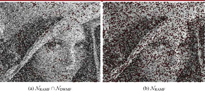
Based on this results, it is proposed to combine the output of two Impulse noise detectors in order to get a more accurate noise estimation whether on a Mixed noise scenario or in a plain Salt and Pepper noise scenario. This approach consists on the combination of the RAMF and the DWMF outputs (denoted asNRAMF∩NDWMF). This filters are chosen based

on the fact that DWMF has a great response for low level Impulse noise inputs, while the RAMF has a good response for high level Impulse noise inputs. This aims to hold the features of both, and thus obtain a high True positives ratio and low false positives ratio for any Impulse noise level and Gaussian Additive noise level.

This novel estimation method is put into test and compared to the RAMF, which is used in the SAIRN algorithm. Both ranked order filters are tested on a Mixed noise scenario for a (256 x 256) patch from (gray) Lena. σ2

η varies within [25510 − 25550] (steps of 25510) and

s within 0% −90% (steps of 0.15). The performance is measured by the true positives and false positives vs. the ground truth noise set each method achieve. Table 4.3 and 4.4 shows the test results. Figure 4.4 shows the false positives forσ2

η = 25510 and s =0.3. The

evaluation shows that the novel approach sustantially decreases the amount of false positives for different s values. Moreover, the true positives almost remain the same in both outputs, which is a favorable feature.

[image:39.595.131.519.227.344.2]

(40)

(a)NRAMF∩ NDWMF (b)NRAMF

Figure 4.4: False positives for (gray) Lena (128×128px.).s= 0.3, σ2_η = ₂₅₅10.

s (elements) σ

2

η=

10

255 σ

2

η=

20

255 σ

2

η=

30

255 σ

2

η=

40

255 σ

2

η=

50 255

R ∩ D R R ∩ D R R ∩ D R R ∩ D R R ∩ D R

0(0) 1269 10920 3101 12512 6279 13222 9063 13769 11207 13928 0.15(10032) 629 5462 1554 6390 3175 6691 4724 6874 5575 6796

0.3(19779) 389 2629 828 2968 1692 3160 2350 3213 2644 3202 0.45(29775) 200 1119 495 1324 743 1221 974 1281 1100 1322

0.6(39399) 85 316 185 380 239 371 296 376 337 402

0.75(49298) 20 60 40 59 47 58 53 65 68 72

0.9(59022) 55 68 59 63 63 68 53 57 88 90

Table 4.3: Impulse noise detectors performance for the Impulse over Gaussian Additive noise scenario: False positives.R:NRAMF,D:NDWMF.

are shown in Figure 4.5. This test images were corrupted with Impulse noise with s = [0.1−0.9](steps of0.2), which matches the experimental setup in [2].

(a) (gray) Bridge (b) (gray) Lena (c) (color) Lena (d) (color) Goldhill

Figure 4.5: Impulse noise scenario test image set.

s (elements) σˆ

2

η=

10

255 σˆ

2

η=

20

255 ˆσ

2

η=

30

255 σˆ

2

η=

40

255 σˆ

2

η=

50 255

R ∩ D R R ∩ D R R ∩ D R R ∩ D R R ∩ D R

0(0) 0 0 0 0 0 0 0 0 0 0

[image:40.595.131.525.69.247.2]

0.15(10032) 9714 9927 9804 9804 9849 9849 9856 9856 10032 10032 0.3(19779) 19779 19779 19625 2968 19710 3160 19607 3213 19702 3202 0.45(29775) 29843 1119 29937 1324 29775 1221 29489 1281 29708 1322 0.6(39399) 39150 39150 39296 39296 39149 39149 39394 39394 39312 39312 0.75(49298) 49201 49201 49007 49007 49038 49038 48991 48991 49298 49298 0.9(59022) 58399 58936 58499 59022 57657 58825 58125 58955 57547 58973