Analysis of multiple change-points in normally distributed series.

i

UNIVERSIDAD AUTÓNOMA DE NUEVO LEÓN. FACULTAD DE CIENCIAS FÍSICO-MATEMÁTICAS.

ANALYSIS OF MULTIPLE CHANGE-POINTS IN NORMALLY DISTRIBUTED SERIES.

Por

JORGE ARTURO GARZA VENEGAS.

Como requisito parcial para obtener el grado de:

ii

ANALYSIS OF MULTIPLE CHANGE POINTS IN NORMALLY DISTRIBUTED SERIES. Chair: Dr. Alvaro Eduardo Cordero Franco.

iii

Table of Contents

Table of Contents ... iii

Abstract ... vi

List of Tables. ... vii

List of Figures. ... viii

Acknowledgments. ... ix

CHAPTER 1. INTRODUCTION TO RESEARCH. ... 1

1.1 History and Background. ... 1

1.2 Problem Statement. ... 4

1.3 Research Questions. ... 5

1.3.1. Research 1: Maximum Likelihood Change-Point Estimators for Normally Distributed Series with Unknown Parameters. ... 6

1.3.2. Research 2: Maximum Likelihood Estimators for Multiple Change-Points. ... 6

1.4 General Hypothesis. ... 7

1.4.1. Research 1: Hypothesis. ... 7

1.4.2. Research 2: Hypothesis. ... 7

1.5 Research Purpose. ... 8

1.6 Research Objective. ... 8

1.7 Delimitations. ... 9

1.7.1. Assumptions. ... 9

1.7.2. Limitations. ... 10

1.8 Relevance of this study. ... 10

1.9 Research Outputs and Outcomes. ... 11

CHAPTER 2. LITERATURE REVIEW. ... 12

2.1. Introduction. ... 12

2.2. SPC and Change-Point Analysis. ... 12

2.3. Literature review for Change-Point Analysis (CPA). ... 13

2.3.1. Parametric Approach CPA. ... 15

2.3.2. Nonparametric Approach CPA. ... 17

2.3.3 General Remarks. ... 18

CHAPTER 3. RESEARCH 1. ... 20

iv

3.2. Background ... 23

3.2.1 Previous Work on Change-Point Analysis ... 23

3.2.2 Q-Charts for Normal Observations ... 26

3.3. Change-Point Estimators ... 28

3.3.1 MLE with ₀ ₁ and ₀ ₁... 29

3.3.2 MLE with ₀ ₁ and ₀ ₁... 30

3.3.3 MLE with ₀ ₁ and ₀ ₁... 31

3.3.4 Change-Point estimation with CUSUM for shifts in mean ... 32

3.3.5 Change-Point estimation with Bartlett’s test statistic ... 32

3.4. Sequential Use of Change-Point Estimators and Control Charts ... 33

3.5. Performance of Estimators ... 33

3.5.1 Retrospective Analysis: Simulation Design ... 33

3.5.2 Online Monitoring with Q-Charts: Simulation Design ... 34

3.5.3 Simulation Results ... 36

3.6. Conclusions and Future Work ... 38

3.7. References ... 39

3.8. Appendix. ... 45

CHAPTER 4. RESEARCH 2. ... 52

4.1. Introduction. ... 54

4.2. Literature Review ... 55

4.3. Model. ... 57

4.3.1. Maximum Likelihood Estimators for shifts in the mean. Case 1. ... 58

4.3.2. Estimators for multiple changes in variance. Case 2. ... 60

4.3.3. Estimators for Shifts in mean and variance. Case 3. ... 61

4.4. Heuristics. ... 62

4.4.1 Greedy constructive heuristic ... 63

4.4.2 Evolutionary Heuristic ... 63

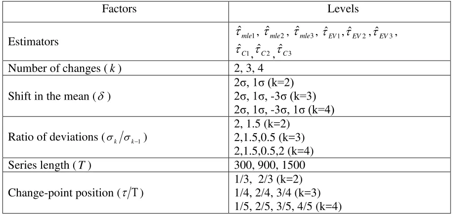
4.5. Experimentation Design ... 66

4.6. Example: measuring the length of a laser scanned object ... 70

4.7. Conclusions ... 71

v

CHAPTER 5. CONCLUSIONS AND FUTURE WORK. ... 76

5.1. General conclusions. ... 76

5.2. Findings from this research. ... 77

5.3. Future Work. ... 79

vi Abstract

This research is composed for two researches which abstracts are:

Paper 1: Change-Point Estimation for a Sequence of Normal Observations and Integration with Q-Charts.

This is the first research regarding to change-point analysis for independent observations normally distributed. It considers the case when a single step change has occurred and

distribution’s parameters (before and after change) are unknown. Development of

maximum likelihood estimators (MLEs) for the change-point and parameters is the main concern as well as an integration with control charts in order to show its application in practice, with which retrospective and on-line analysis are both covered. A change is considered as one of the three different cases: (1) change only in mean parameter, (2) change only in variance parameter or (3) change in both parameters. Due to there are change-point estimators for change in mean and change in variance, comparison is done to show what estimator is recommended to use in each situation.

Paper 2: Estimation of multiple change-points in time series normally distributed using a construction Heuristic and a Genetic Algorithm.

This is the second research related to change-point analysis for independent observations normally distributed. It considers case when multiple step changes have occurred assuming

vii List of Tables.

Table 1. Summary of CPA literature review. ... 15

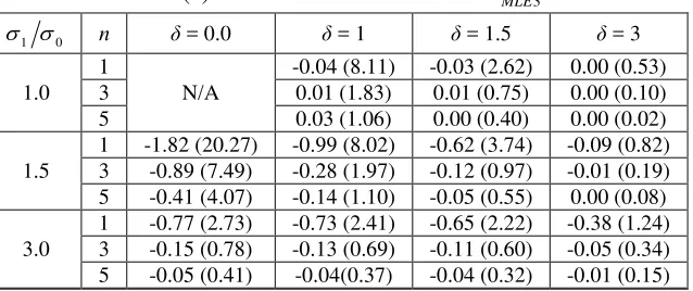
Table 2. Performance of change-point estimators when ₀ ₁ and ₀ ₁. ... 45

Table 3. Performance of change-point estimators when ₀ ₁ and ₀ ₁ ... 46

Table 4. Performance of change-point estimators when ₀ ₁ and ₀ ₁ ... 47

Table 5. Performance of change-point estimators when ₀ ₁ and ₀ ₁ ... 48

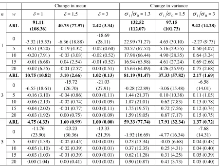
Table 6. Performance of change-point estimators for on-line analysis for changes in mean and changes in variance, respectively. ... 49

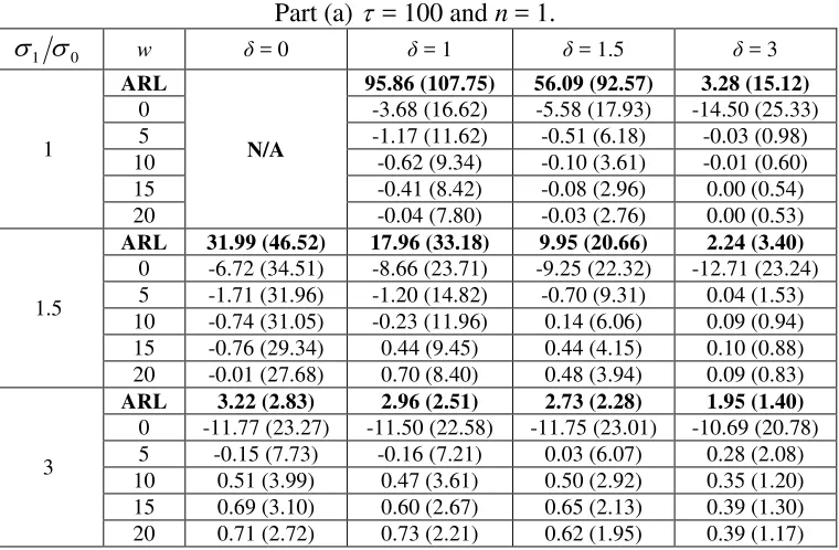
Table 7. Performance of change-point estimators when ₀ ₁ and ₀ _{1 , for on-line} monitoring. ... 50

Table 8. Factor to measure the performance of change-point estimation ... 66

Table 9. Performance of multiple change-point estimators for k 2 changes. ... 67

Table 10. Performance of heuristics for multiple change-point estimators for k3 changes. ... 68

Table 11. Performance of heuristics for multiple change-point estimators for k 4 changes. ... 69

viii List of Figures.

Figure 1 Control charts for a time series with a change in the mean. ... 2

Figure 2. Types of changes studied in CPA. ... 3

1

CHAPTER 1. INTRODUCTION TO RESEARCH.

1.1History and Background.

Every process has variation, which could be left to a chance or be attributed to assignable causes. According to Shewhart's (1931) third postulate assignable causes must be found and eliminated in order to secure a statistical control state: This provides advantages such as reduction in the cost of inspection and the cost of rejection. Thus, this way of management has two aspects: first, the detection of special causes of variation and second finding and eliminating these to bring the process back to control. As soon as the assignable causes are detected, the process will improve. Several tools and procedures have been developed in order to assist in the management of systems; one of the best known tools are control charts that are capable of determining whether or not the process is in statistical control. Nevertheless, when sustained changes have occurred, most of control charts are not able to determine the initial moment of the change, which provoke delays in the application of corrective actions. Change-point analysis is the study of structural changes in series of observations. The problem of estimating the moment of a change is called the change-point problem. Several control charts and change-point estimators have been created by assuming a priori knowledge of distribution parameters while, in practice, this assumption is not always met. In consequence, it seems reasonable to develop such tools.

Control charts were first developed by Shewhart (1931) to determine whether or not variability could be left to chance or common causes. Since then, several control charts have been developed keeping the same objective. Control limits are calculated based on rules provided by the control chart itself, then data or a transformation is plotted with corresponding control limits. If one or more observations fall outside control limits, the chart is said to signal the presence of a potential change in the process and as a consequence, variation could be attributed to special causes, otherwise process’ variation is left to chance.

2

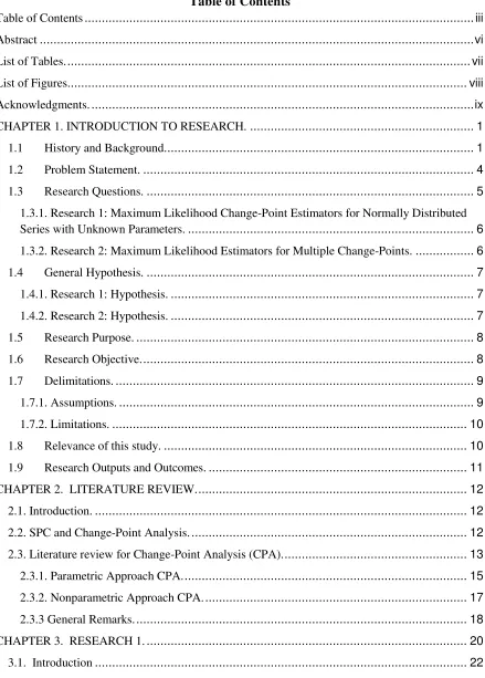
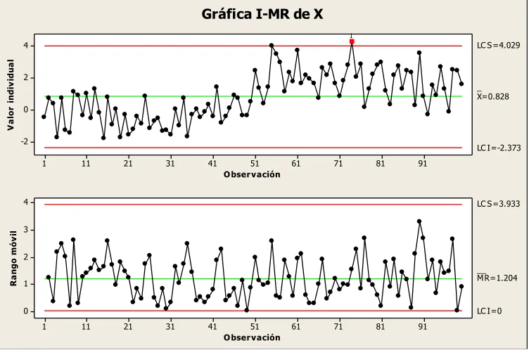
within them, and sustained, which is considered a change in the process distribution characteristics over the next outputs. As it was mentioned, control charts are not usually capable of estimating (estimation is always positively biased) the initial moment when a sustained change occurs. For instance, Figure 1 shows a shift in the mean at 50th observation while the chart detects it until 73rd observation. This delay represents a problem for managers because this signal is away from the real moment of the change and

the process’ improvement might be retarded which means misspending resources.

91 81 71 61 51 41 31 21 11 1 4 2 0 -2

O bser vación

V a lo r i n d iv id u a l _ X=0.828 LC S =4.029

LC I=-2.373 91 81 71 61 51 41 31 21 11 1 4 3 2 1 0

O bser vación

R a n g o m ó v il __ M R=1.204 LC S =3.933

LC I=0

1

Gráfica I-MR de X

Figure 1 Control charts for a time series with a change in the mean. (Chart created using Minitabtm_).

3

and Zamba (2005a) developed a change-point estimator with no assumption of prior

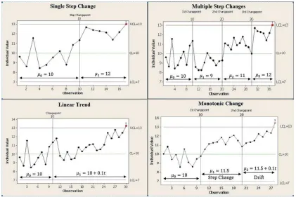
knowledge of parameters using a statistic based on Bartlett’s test. Recently, Amiri and Allahyari (2011) catalogued changes in the following 4 categories: single step changes, multiple step changes, changes with linear trend, and monotonic changes; they are presented in Figure 2.

Figure 2. Types of changes studied in CPA. Image obtained from Amiri and Allahyari (2011).

Other problem that was addressed is the case of multiple change points for which Perry, Pignatiello, and Simpson (2007, p.328) proposed that “… this type of behavior might occur

4

Since the knowledge of time when the change occurred might boost an improvement process and reduce the cost of rework, waste and downtime, this research aims to develop change-point estimators without assuming prior knowledge about parameters before and after sustained changes occurred using the Maximum Likelihood Method. In addition, estimators for cases where more than one sustained change occurred in mean and/or variance of normal processes will be derivate in order to assess the problem defined by Perry et al. (2007).

1.2Problem Statement.

Shewhart’s Third Postulate for Control states that assignable causes of variation may be identified and therefore eliminated, which is desirable to maintain a state of control (Shewhart, 1931). The following two major advantages are obtained: reduction in costs of inspection and rejection. This research addresses the problem of estimating changes moments in time series, in order to reduce the time required to look for assignable causes of variation to help reduce cost of inspection, rejections, and downtime. One approach to address this problem is by obtaining estimators of the change-points that have occurred. This also could answer a question previously proposed by Arunajadai (2009, p.58): “Are

the data homogeneous and if not, what are the locations of the homogeneous segments in the data?”

For a single sustained change, most approaches suppose previous knowledge of initial parameters (when in practice in several cases this is not true, for instance, in Phase I of SPC), while, in this research, this assumption is not considered. Change-point estimators when parameters (before and after sustained changes occur) are unknown will be developed by using maximum likelihood methodology due to maximum likelihood estimators (MLEs) provides the more likely values of the true parameters according to all available information. Assumptions made by the proposed solution model are that changes had really occurred and data is normally distributed. A change-point of the series (or process) is

5

addressed: (1) Change only in mean, (2) change only in variance and (3) change in both parameters at the same time. The results of this approach will be compared with those found in the literature in order to evaluate their performance in terms of accuracy and effectiveness in order to determine which estimator is recommended to use in each situation.

Situations where a process is out of control and multiple change-points have occurred has been worked mostly through applications for shifts in the mean and Bayesian approach as can be found in Fotopoulos, Jandhyala, and Khapalova (2010). In this research MLEs for multiple change-points are developed as well as two heuristics algorithms (evolutionary and constructive) to avoid computational cost due to change-points MLEs time required to obtain them increases in a non-polynomial way which could lead in a retard in searching assignable causes of variation. Similarly to one sustained change, three cases are considered in this problem: (1) k changes only in mean, (2) k changes only in variance and (3) k changes in both parameters at the same time. Finally, simulation will be performed in order to show the behavior of these estimators.

1.3Research Questions.

This research is two folded: the first one is focused on single step change-point problem, and second one, on multiple step changes. Since previous works in literature usually assume prior knowledge of parameters, it follows that:

 Q.1. Does maximum likelihood change-point estimators exist when there is not previous knowledge of parameters for time series normally distributed in which k sustained changes occurred? This is not a trivial question, since MLEs do not always exist.

6

1.3.1. Research 1: Maximum Likelihood Change-Point Estimators for Normally Distributed Series with Unknown Parameters.

In this research, change-point MLEs were developed for time series normally distributed with a single step change, considering three different cases: (1) change only in mean, (2) change only in variance, (3) change in both parameters at the same time. Change-point estimators found in literature, which are sensitive to: shifts in the mean (CUSUM estimator; Pettitt, (1980)), and shifts in variance (Hawkins and Zamba, (2005a)), were used to compare with. Finally, integration with Quesenberry’s Control Charts (Q-charts) (Quesenberry, 1991a, 1991b, 1991c) is presented in order to show its application in on-line monitoring. The sub-questions addressed in this research are:

 Q.1.1. What is the bias and spread of estimators in cases (1), (2) and (3)?

 Q.1.2. In which scenarios MLEs’ performance is better than CUSUM and Hawkins estimators by means of accuracy and effectiveness?

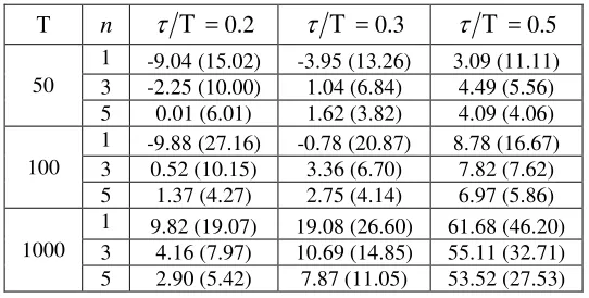
 Q.1.3. What is the bias and spread of the change-point MLEs after signals of Q- Charts?

1.3.2. Research 2: Maximum Likelihood Estimators for Multiple Change-Points.

In this research, change-points MLEs for time series with multiple changes were developed as well as heuristic (evolutionary algorithm) and constructive algorithms to assess the problem of finding MLEs, which is a non-polynomial (NP) optimization problem. Three cases are considered: (1) k changes only in the mean, (2) k changes only in variance and (3) k changes in both parameters at the same time. Performance of MLEs and heuristics is shown by considering few scenarios. Questions:

 Q.2.1. Is the multiple change-point estimation obtained by the Maximum Likelihood methodology solving time increasing in a non-polynomial way as number of changes increases?

 Q.2.2. What is the bias and spread of estimators in cases (1), (2) and (3)?

7

1.4General Hypothesis.

The general hypothesis of this research is:

 H1. It is possible to develop the change-point (single or multiple) maximum likelihood estimators for parameters as well as for change-points when prior knowledge of parameters does not exist.

1.4.1. Research 1: Hypothesis.

The following hypotheses are proposed for research 1:

 H1.1. Bias and spread of change-point MLEs tends to be smaller compared to CUSUM and Hawkins ones when change in both mean and variance occurred at same time. When there is only change in mean or only change in variance, CUSUM and Hawkins estimators biases and spread tends to be smaller than its corresponding change-point MLEs.

 H1.2. Change-point MLEs’ performance is better than CUSUM and Hawkins performance when size of the series is big in means of bias and spread.

 H1.3. Change-point MLE’s performance is precise and accurate when it is used

after a Q-chart signal.

1.4.2. Research 2: Hypothesis.

The following hypotheses are proposed for research 2:

 H2.1. The problem of finding multiple change-point MLEs correspond to optimization problem because of solving time increases in a non-polynomial way.  H2.2. What is the bias and spread of estimators for cases (1), (2) and (3)?.

8

1.5Research Purpose.

This research is mainly focused on developing change-point estimators for single and multiple step changes for normally distributed series. These estimators are expected to be as close as possible to the true change-points locations. Even though there are estimators for such data yet, the case when parameters (before and after the change) are unknown has been almost not worked in literature, and that case could be presented in practice. Moreover, by showing that these tools have less bias and spread in several scenarios than others estimators found in literature, particularly, Pettit’s CUSUM (1980) for shifts in the mean and Hawkins’ (2005a) estimators for shifts in variance.

In other words, development of tools for system management which could help in identification of assignable/special causes of variation which might be eliminated according to third postulate of quality (Shewhart (1931)) is the main purpose. Determine whether or not a process is in control is a task relegated to control charts, as it can be seen with

change-point MLE’s integration with Q-charts.

1.6Research Objective.

Let xi,jbe random variables following:

                   

 if i T j n

n n j i if n n j i if n x m m m j i 1 ; ) , ( 1 ; ) , ( 1 ; 1 ) , ( ~ 2 1 1 2 1 2 2 2 1 2 1 1 ,            (1)

Where _k for k 1,2,...,m are called the series’ change-points; j is the number of replications and , 2for _1,2,..., _1

m r

r r 

 are the parameters of the normal distribution in

9

Objective 1: Derive the change-points MLEs ˆ₁,ˆ₂,...,ˆ_k  for change-points of the series  1,2,...,k  for different cases:

Case 1: ; ... 2 2; 1,2,..., .

1 2

2 2 1

1 m p k m

k

k          

 (2)

Case 2: ; 2 ; 1,2,..., .

1 2

1 k k k m

k

k        

 (3)

Case 3: ; 2 ; 1,2,..., .

1 2

1 k k k m

k

k       

 (4)

Objective 2: If k 1, show that change-point MLE ˆ for (2), (3) and (4) bias and spread

tends to be lower as size of the series increases. Also show that change-point MLE (4) is more precise and accurate than Pettitt’s (1980) CUSUM and Hawkins’ (2005a) estimators. Objective 3: If k 1, show change-point MLE ˆ integration with Q-charts.

Objective 4: If k 1, show that change-point estimation is a NP Problem.

Objective 5: Develop heuristics for multiple change-points MLEs.

τbjective 6: Show that heuristics’ performance is similar to MLEs (in cases where they could be compared).

1.7Delimitations.

The next sub-sections present the assumptions and limitations addressed by them.

1.7.1. Assumptions.

The following assumptions were made in the model:

1.- Observations are independent random variables following (1).

2.- It is known a priori that kchanges have already occurred over the process.

3.- It is considered that a change have occurred when one or both parameters distribution change.

4.- Parameters before and after each change-point as well as change-points locations are unknown.

10 1.7.2. Limitations.

Under assumptions made above, the following limitations appear:

With assumption of prior knowledge of that k changes have already occurred, three limitations addressed:

 It is necessary to know the number of changes that have occurred in order to obtain better estimations by using this procedure. Due to control charts only could help to determine if the process is out of control but are not capable to ensure that changes have already occurred.

 When changes have occurred and the control chart signals that, they not provide a clue of the type of change, thus, changes with trend are not covered, such as the case when machines wear out.

 Even when a control chart provides a signal of a process out of control, this signal could be a false alarm, but change-point estimators always determine a point of the time series of where it is more likely that the change have occurred according with the information provided. That is, this procedure could lead to an estimation of change-points, but this “change” could not be considered as statistically significant.

There are some techniques which could help to estimate the number of changes in a time series, like CUSUM control charts of Page (1954). Nevertheless, this research assumes prior knowledge of the number of changes. Finally, hypothesis test is recommended to use to determine if there is a significant change-point in the series, but it is left as future work because it is beyond the research scope. It is noteworthy that normality assumption is not senseless because in practice, the data collection is often with replications, and then limit central theorem ought to be applied.

1.8Relevance of this study.

11

before. Maximum likelihood procedure was chosen because of its properties: they provided the most likely value of the parameters under estimation, and they are asymptotically unbiased, that is to say, if sample size tends to infinity, then estimator tends to be unbiased.

Multiple change point problem has many applications in natural phenomena and Medicine as can be found in Arunajadai (2009) and Fotopoulos et al. (2010). However, almost all of the cited works there were done from a Bayesian approach, and maximum likelihood procedures were almost not found in literature.

Even though control charts are important because they are useful to determine whether the process is in control, they are not capable to determine the change-points, which could retard the process improvement and leads in a waste of resources. Nonetheless, without that information provided by them no inferences about the change-point could be determined. This suggests that both tools should be used in a complementary way. So, change-point estimators boost the improvement process by giving one location in which start to searching special/assignable causes of variation. That is why integration with these estimators with Q-charts is presented as usefulness and necessary tools.

1.9Research Outputs and Outcomes.

The major output of this research is the procedure to assist process management when there is not prior knowledge about distributions parameters, that is to say, Phase I of SPC. The following outcomes will be addressed:

1. – Change-points MLEs.

2. – Integration of change point MLE’s with Q-charts giving a procedure to system managers.

3. – Multiple change-point estimations by heuristics based on MLE’s in order to avoid the

computational time problem addressed in this case.

12 CHAPTER 2. LITERATURE REVIEW.

2.1. Introduction.

Statistical Process Control (SPC) is used to reduce variation leading to improvement in the performance of processes (Amiri and Allahyari, 2011) .There are two phases in SPC: Phase I in which parameters are estimated with historical data assuming that process is in statistical control whereas in Phase II the process is monitored: new data is tested to being in control according to information provided in the previous phase. Most common tools used in Phase II are control charts which use was explained in previous chapter Phase II is monitoring phase in which it is desirable to determine whether a change have occurred. Amiri and Allahyari (2011) classified different types of changes that have been studied, in which process get out of control: step changes, multiple step changes, changes with drift and monotonic changes which are a mixture of latter ones. In this section, it will be shown the connection of SPC and Change–point analysis going through those techniques and approaches used before CPA was defined and later.

2.2. SPC and Change-Point Analysis.

First tools developed under SPC label were control charts, which are tools that are used to monitor a process and detect assignable and special causes of variation Amiri and Allahyari (2011). Control limits are calculated and then when one or more than one observations fall outside that limits, then it is suspected that a change occurred. In 2007, Koutras, Bersimis, and Maravelakis (2007) classified control charts in 3 major categories: (1) Shewhart’s

13

ones, EWMA’s control charts, assign larger weights to new observations in order to avoid no detections of small shifts.

All of these tools are good determining whether or not the process is under statistical control (which is the first step at system management), but when the process is out of control, it is desirable to know at which moment that happened and then apply corrective actions, and control charts have a delay at reporting that in almost all cases. The search of this moment is called change-point problem and change-point analysis was defined by Potts (2003) as a method to find thresholds in relationships between two variables. Taylor (2000) shows differences between use of control charts and CPA (the first one controls point-wise error rate while last ones, the change-wise error rate) and how they can be used in a complementary way in SPC.

2.3. Literature review for Change-Point Analysis (CPA).

Change-point problem was firstly worked, from a Bayesian approach, by Girshick and Rubin in 1952. They proposed quality control rules which have to be applied after a change in a random process was detected. Problem of determine the initial moment of a change has been worked from several approaches: parametric, non-parametric, Bayesian and regression. From parametric approach, almost all works found are about developing

MLE’s, control charts and tests based on Likelihood Ratio (LR) tests. On the other hand, from a nonparametric approach, transformations of data to another with known distributions were worked. These works are detailed in the next subsections but summarized in Table 1.

Approach Author(s). Contributions.

P

ara

metric

Page (1954) CUSUM charts.

Hinkley (1970)

Developed change-point MLE for change in process mean and a statistic. Also derived their asymptotic distributions.

Hinkley (1971) Derived asymptotic distribution of CUSUM estimator as well as of its statistic.

Samuel, Pignatiello, and Calvin (1998a)

Change-point MLE using Shewhart’s Xcontrol

14

Samuel, Pignatiello, and Calvin (1998b)

Change-point MLE for a change in variance using S or R control charts.

Samuel and Pignatiello

(1998) MLE for Poisson parameter.

Timmer, Pignatiello, &

Longnecker, (1998) Control chart for changes in AR(1) time series.

Jann (2000) Change-point estimator for multiple changes in normal processes with shifts in the mean using a genetic algorithm.

Dabye and Kutoyants

(2001) MLE for Poisson using boundaries.

Samuel and Pignatiello

(2001) MLE for binomial’s p parameter.

Nedumaran, Pignatiello

and Calvin (2002) MLE for changes in mean of Normal Multivariate processes. Timmer and Pignatiello

(2003) MLE for changes in AR(1) processes.

Hawkins and Zamba (2005a)

Control chart based on GLR test using Bartlett’s

test for changes in variance. Parameters unknown.

Zamba and Hawkins (2006)

Control chart based on LR test for change in mean of multivariate normal processes. Liming (2008) MLE for autoregressive time series. Reynolds and Jianying

(2010)

Control chart based on GLR for shifts in the mean of normal processes.

Fotopoulos (2010) Derived the exact asymptotic distribution of change-point MLE in a computable form.

Cordero et al. (2012) Control chart based on 2test for changes in variance.

Tercero et al. (2012) Control chart for change in variance based on F _test.

Chen and Gupta (2012) Compiled Parametric CPA works.

Tercero et al. (2013a) Integration of change-point MLE with a self-_{starting CUSUM for normally distributed series.}

Non

-P

ara

metri

c Page (1955)

Use the sign function to determine changes in the known initial mean parameter for symmetric distributions.

Bhattacharyya and

Johnson, (1968) Test for shift in the mean of observations which has a symmetric cumulative distribution. Pettitt (1979) Nonparametric test for Bernoulli, Binomial or

continuous distributions.

15

Hinkley, D. V., and

Schechtman, E. (1987) Bootstrap method for shifts in the mean process.

Ghazanfari, et al. (2008)

Clustering technique to estimate change-points for normal or non-normal distributed time series with shifts in the mean.

Ghazanfari, M., Alaeddini, A., and Noghondarian, K. (2008)

Clustering method capable to estimate change-points and parameters values after a change in the mean.

Harchaoui, Bach, and

Moulines (2009) Test statistic for homogeneity of two-subsamples and derived its asymptotic null distribution Tercero, G., Temblador,

M., Beruvides, M. and Hernández A. (2013b)

Change-point estimator using p-value of Mood’s

median Test for random walks with drift. Table 1. Summary of CPA literature review.

2.3.1. Parametric Approach CPA.

Page (1954) started this line of research with his CUSUM control charts. Even though this procedure dos not estimate the initial moment of a change, gives a signal that a change have already occurred (Tercero (2011)). MLEs were considered by first time for Hinkley (1970). He developed MLEs for changes for independent random variables normally distributed for Phase II of SPC as well as LR tests. After that, Hinkley (1971) derived the asymptotic distribution of the MLE for changes in the mean when parameters are known or unknown, but it was not presented in a computable form. This could be considered as the base work. Next works are presented in three different categories: Estimation, Control Charts, and Ratio Tests.

Change-point MLEs following Hinkley’s (1971) guideline were developed by the following authors. (Samuel, Pignatiello, and Calvin, 1998a) developed change-point MLE for a change in the mean of normally distributed data which is used after a signal of a

16

performance over different subgroup sizes and changes in variance measured in ratio of deviations.

Change-points MLEs for other distributions were also developed. Samuel and Pignatiello (1998) proposed an estimator for a step change in a Poisson rate parameter, using the same analysis of their previous works. Dabye and Kutoyants (2001) also worked with this distribution but they demonstrate consistency of the change-point MLE by considering boundaries. MLE for Binomial distribution p parameter was developed by Pignatiello and Samuel (2001) and its performance was evaluated after a signal given by a p or np chart along different values of p. For multivariate normal process with a change in mean, Nedumaran, Pignatiello and Calvin (2000) developed the change-point MLE and evaluated its performance over different scenarios. Liming (2008) proposed some statistic for change-point problem for autoregressive time series models with both cases of variance known or unknown.

Control charts integration with change-point estimators were first done by Timmer, Pignatiello, and Longnecker (1998), they proposed a test for monitoring the level parameter of AR(1) processes which resulted in a CUSUM-based control chart. Later, Timmer and Pignatiello (2003) proposed three estimators for the parameters of such that model, using their previous control charts. Reynolds and Jianying (2010) developed a control chart using a moving window based on GLR methodology for small shifts in the mean of normally distributed data. Using GLR, Cordero et al. (2012) and Tercero et al. (2012) developed control charts and change-point estimators for changes in variance in normally distributed

data using the F test and the 2test for Phases I and II, respectively. In 2013, Tercero et

al. (2013a) integrated the change-point MLE for shifts in the mean after a signal of a self-starting CUSUM.

Hypothesis tests were worked by several authors after Hinkley’s (1970) work. Hawkins and Zamba (2005a) developed a LR test based on Bartlett’s test for mean and variance of

17

variance or both parameters. After that, Zamba and Hawkins (2006) developed a LR Test for multivariate normal processes with shifts in the mean. Fotopoulos et al. (2010) continued Hinkley’s (1970) work and derived the exact asymptotic distribution of the MLE for changes in the mean as well as the LR Statistic obtaining good approximations of the actual MLE distribution.

Several parametric CPA works were compiled by Chen and Gupta (2012) in 2012, including estimation, LR tests, and change-point null distribution. This monograph also includes applications of CPA for single and multiple change-point problems.

2.3.2. Nonparametric Approach CPA.

Assesing the problem from a nonparametric perspective, Page (1955) proposed a method to identify changes in the process mean where initial parameter was known using the sign

function:y_i sgn





18

Alaeddini, and Noghondarian (2008) devised a new clustering method capable to estimate the time at which a sustained shift in the mean occurred as well as for true values of the out

of control process’ parameters. Based on the maximum kernel Fisher discriminant ratio Harchaoui, Bach, and Moulines (2009) proposed a test statistic which was developed as an indicator of homogeneity of two sub-samples, and, when this statistic indicates that a change have occurred also gives an estimation of the change-point. They derive the asymptotic distribution of their statistic under null hypothesis of no change as well as its consistency under alternative hypothesis of change. Recently, Tercero et al. (2013b) developed a change-point estimator for random walks with drift using the p-value of the

Mood’s median test.

2.3.3 General Remarks.

There are several approaches to solve the change-point problem as well as types of changes: single step changes, multiple step changes, changes with linear trend, and monotonic changes according to Amiri and Allahyari’s (2011) literature review. This research considers only parametric approach for single and multiple step changes in time series. Under this label, many approaches of solution suppose initial parameters as known; other works have approximate or asymptotic results for the estimator’s distributions.

19

About multiple change points, according to Jann (2000) and Fotopoulos et al. (2010) there are several researches focused mainly in application of CPA like meteorology, analysis of DNA sequences, signal processing, econometrics, and statistical process control. A vast number of researches were found for climate data analysis trying to find change-point in rainfalls records (or find inhomogeneities in climatological time series): Potter (1981), Maronna and Yohai (1978), Easterling and Peterson (1995), Lanzante (1996), Alexandersson and Moberg (1997). For DNA sequences, Arunajadai (2009) presents a

methodology to model the RσA unwinding mechanism using Tukey’s biweight function to detect changes in the mean. Fu and Curnow (1990) studied Bernoulli independent variables sequences, and derived the MLE distribution of the location of two changed segments to predict protein helical regions. Finally, tests for multiple change-point have been developed by Huskova and Slaby (2001), and Aly, Abd-Rabou and Al-Kandari (2003).

20 CHAPTER 3. RESEARCH 1.

Change-Point Estimation for a Sequence of Normal Observations and Integration with Q-Charts

This is the first research of change-point analysis for independent observations normally distributed. It considers the case when a single step change has occurred and distribution’s

parameters (before and after change) are unknown. Development of maximum likelihood estimators (MLEs) for the change-point and for parameters is the main concern as well as an integration with control charts in order to show its application in practice, with which retrospective and on-line analysis are both covered. A change is considered as one of the three different cases: (1) change only in mean parameter, (2) change only in variance parameter or (3) change in both parameters. Due to there are change-point estimators for change in mean and change in variance, a comparison is done to show what estimator is recommended to use in each situation.

21

Change-Point Estimation for a Sequence of Normal Observations and Integration with Q-Charts.

Víctor G. Tercero-Gómez, Ph.D, Alvaro E. Cordero-Franco, Ph.D, Jorge A. Garza-Venegas, B.S., María del Carmen Temblador-Pérez, Ph.D., Mario G. Beruvides, Ph.D.

Many practical applications have to deal with situations where parameters are unknown and have to be estimated from collected data where a structural change happened at an unknown change-point. This situation is found during start-up processes, root cause analysis performed over past observations, and many other situations where backward-looking examination for a change-point in some measured variable is required. This paper presents and evaluates the performance of three maximum likelihood estimators (MLE) of the change-point in series for retrospective analysis and online monitoring through the sequential use with Q-charts. Process parameters, before and after a change, are assumed to be unknown. Different shifts, sample sizes, and locations of change-points were evaluated. For retrospective analysis, a comparison is made with estimators based on cumulative sums and

Bartlett’s test. Performance analysis done with extensive simulations showed that the MLEs perform better (or equal) in almost every scenario, with smaller bias and standard error. Integration with Q-charts showed that the sequential use of both methodologies facilitates the detection and estimation of special causes of variations, fostering any quality improvement effort. Strategies to reduce bias and standard error of estimators through the use of additional observations are also presented.

22 3.1. Introduction

Control charts are known tools to detect isolated and sustained changes. However, when sustained changes occur, most of them are not capable of estimating the initial moment of the change. Knowing this exact time greatly simplifies the search for a cause of variation, and in consequence, might boost an improvement process. The search for this moment is called change-point estimation. Potts (2003) defines it as methods created to identify thresholds in the relationship between two variables; however, it can be generalized for multiple changes. From a parametric point of view, following the guidelines of Hinkley (1970), several authors like Samuel et al. (1998a) and Khoo (2004) have studied the behaviour of the maximum likelihood estimators (MLE) for a change-point of a normal process. These authors studied the behaviour of these estimators where a priori knowledge of initial parameters existed. Nevertheless, real life applications usually lack this information, and parameters have to be estimated from collected data.

This research is focused on the construction and performance evaluation of several change-point MLEs for normal observations collected over a discrete time where parameters before and after the change-point are unknown. Given a time series of independent observations

n n

n

n X X X X X X

X

X_1,1,..., _1, ,..., _,1,..., _, , _1,1,..., _1, ,..., _,1,..., _, following the subsequent

model:









1 , , , 1 , 1 , , ~ 1 1 0 0 , _{  }    (1)

Where parameters , ₀, ₁, ₀ and ₁ are unknown.  is called the change-point of the

series, and  is the last sample observed. To estimate the change-point, three MLE estimators called ˆMLE1, ˆMLE2, and ˆMLE3 are obtained based on three different scenarios,

according to different assumptions about parameters of the normal distribution.

1

ˆMLE

 assumes that ₀ ₁ but ₀ ₁.

2

ˆMLE

 assumes that ₀ ₁ but ₀ ₁.

3

ˆMLE

23

To measure the performance of these estimators, this research evaluated, with extensive simulations, different scenarios where the size of the shift, sample size, and the change-point position were modified to measure the sensitivity of estimators. Results are compared with estimators from Pettitt (1980) and Hawkins and Zamba (2005a). Additionally, to extend the applicability of the proposed estimators, integration with Q-charts is proposed and their performance is evaluated.

Section 3.2 presents an overview of the research in change-point analysis, and briefly describes Q-charts with their related literature. The research showed no indication of the existence of an in-depth study of the biases and errors of the proposed estimators when applied in retrospective analysis for limited sample sizes. Neither was any study found about their performance when used sequentially with Q-charts. Section 3.3 presents the proposed change-point estimators. Section 3.4 shows how change-point estimators can be integrated with Q-charts. Experimental results from Monte Carlo simulations are described in Section 3.5; and finally, some general conclusions and opportunities for future research are mentioned in Section 3.6.

3.2. Background

3.2.1 Previous Work on Change-Point Analysis

Concerns of detecting sustained changes in time series started with Girshick and Rubin (1952) from a Bayesian paradigm. They defined a quality control rule to trigger corrective actions when a change in a random process was detected. Soon after, Page (1954, 1955, 1957), from a frequentist point of view, developed the cumulative sum (CUSUM) chart to be able to detect, faster than traditional Shewhart's control charts (1931), the presence of sustained changes.

24

(2002), Timmer and Pignatiello (2003) and Liming (2008) developed MLEs for series following different distributions. They focused their work on the integration with control charts, where the MLEs were used as a plug in to estimate the change already detected. To detect if a change had happened, Timmer, Pignatiello, and Longnecker (1998) worked on a LR test based on the CUSUM chart to detect changes in a first order autoregressive process. Hawkins and Zamba (2005b), and Zamba and Hawkins (2006) and Batsidis (2010) worked on several LR tests to make inferences whether a change has occurred in individual stationary series. Hawkins and Zamba (2005a) presented a model to deal with variance changes, similar to the generalized likelihood ratio (GLR) control chart for variance, based

on Bartlett’s test. σevertheless, the proposed model grew in complexity as more

observations were added into the time series. To solve the complexity issue of the GLR when dealing with mean changes, Reynolds and Jianying (2010) simplified the approach by suggesting the application of a moving window, where the amount of steps required with each new observation was restricted to the size of the window.

Aside from MLE procedures, Ghazanfari et al. (2008) proposed the use of clustering principles to identify two partitions, within the time line, where the probability of an observation of belonging to one of the two sets in the series was used as a separation criterion. Page (1954), when developing the CUSUM, first pointed that results from this technique could be used to estimate the initial time of the change. Hinkley (1971) compared the later estimation with the MLE for known initial parameters of normal and independent observations, concluding that the use of the CUSUM is asymptotically biased, but easier to use. Pettitt (1980) proposed the estimation with CUSUM for unknown parameters, and Nishina (1992) evaluated the performance against estimations obtained from EWMA and Moving Average charts, determining that estimation from CUSUM was superior, and, if the size of the change is known a priori, he proved that the estimation with the CUSUM was an MLE.

25

Wang (2006), Perry, Pignatiello, and Simpson (2006), Mahmoud, Parker, Woodall, and Hawkins (2007) and Zhou, Zou, Zhang, and Wang (2009). All of these tests assumed normally distributed errors and were designed to detect changes in the intercept and the slope of trended series.

On the other hand, Bayesian statisticians continued with the research line initiated by Girshick and Rubin (1952). For stationary observations, several approaches were proposed by Shiryaev (1963), Chernoff and Zacks (1964), Barry and Hartigan (1993), Chib (1998) and Moreno, Casella, and Garcia-Ferrer (2005). For non-stationary observations, Ferreira (1975) developed an estimator and confidence intervals for the change-point of trended observations with normal errors. Holbert (1982) and Chen (1998) also worked with change-point analysis for multiple linear regression models. Finally, Western and Kleykamp (2004) designed a change-point estimator for the coefficients of a regression line using simulation methods.

Bhattacharyya and Johnson (1968) were responsible for the first construction of a nonparametric test with the explicit idea of doing a nonparametric method. However, Page (1955) was the first one to develop a nonparametric change-point detection technique. He applied the CUSUM technique to the dichotomy created by the sign of the difference between observations in a time series and a specification. Later, Pettitt (1979) used nonparametric techniques to change-point analysis by developing tests for Bernoulli, binomial and continuous observations. A year after, Pettitt (1980) approached the CUSUM for zero-one observations, similar to the one built by Page (1955). Finally, Hinkley and Schechtman (1987) applied the re-sampling technique, the bootstrap, to estimate the moment of a shift in the mean. Tercero et al. (2013b), also from a nonparametric perspective, using the p-value of Mood’s median test (1954), constructed an estimator capable of detecting changes in the median of time series. Recently, Zou et al. (2007) proposed the use of the empirical likelihood ratio to approach the change-point test and estimation problems.

26

invertible ARMA processes. Latter, Perry (2010) derived and evaluated the MLE for the time of polynomial change in mean of covariance-stationary autocorrelated process. Finally, Perry and Pignatiello (2012) obtained a MLE for the change point in the fixed-effects components in a two stage-nested random model.

For series of normally and independently distributed observation, many MLEs for known parameters have been developed and studied. However, when dealing with real life situations, parameters are usually unknown. Even when parameters are assumed to be known, most of the time they were estimated from historical data. From the reviewed literature, change-point estimation for unknown parameters hasn’t been deeply studied, and

its construction and performance needed to be addressed. The following section introduces the MLEs for unknown parameters under three different circumstances when mean and variance are assumed to be equal or different. Pettitt (1980) and Hawkins and Zamba (2005a) estimators are also presented.

3.2.2 Q-Charts for Normal Observations

27

no assumptions about none of the true values of parameters in normal sequences of independent observations. These are the control charts for mean and variance for individual observations and rational subgroups where samples have at least two observations each. Charts formulas are shown in equations (2-11).

Q control chart for individual observations. Here r stands for the moment in time.

r x x r i i r



 1 (2)







 

1 1 2

1

2

1 _{ }

                                    r s x x r r G x Q r r r r r r (4)

Where G_r2 and 1 are for the t distribution with r – 2 degrees of freedom and the inverse normal standard distribution.

Q control chart for mean using rational subgroups.

r r i i i r n n x n x   







p _{  }

 







1 _{ }

        _          r p r r r r r r s x x n n n n n n n

W (7)

 



 



     _{   } r n n n r

r x G W

Q

r (8)

Q control chart for process variances with individual observations

1  

 _{r r}

r x x

28

 

2 .; , 6 , 4 r , 2 2 2 4 2 2 2 , 1

1 _{  }

                     r R R R R F R Q r r r r      (10)

Q control chart for process variances using rational subgroups.













1 1 2 1 1 2 1 1 1 ... 1 1 ...             r r r r r s n s n s r n n W (11)

 



 



1 2

1   



  _{     }

 r r n

n n n r

r s F W

Q

r

r (12)

Q-charts belong to the area of self-starting control charts. This type of control charts deal with the problem of monitoring processes without the need of a previous estimation of process parameters. This problem was first assessed by Hawkins (1987) by adapting the CUSUM chart to include running estimators of mean and variance. Later Quesenberry (1991a, 1991b, 1991c) used this approach to create self-starting Shewhart-type control charts (as previously presented) for Normal, Binomial, and Poisson observations. Zou et al. (2007) applied linear regression results to develop a self-starting control chart to monitor several related variables called linear profiles. He et al. (2008) proposed a different running estimator of the variance to reduce the bias of Q-charts when a change happened early (a bias occurs when the out-of-control ARL is larger than in-control ARL when a change does exist). To improve power of self-starting charts, Capizzi and Masarotto (2012) used EWMA statistics over Quesenberry´s Q variables, and applied a CUSCORE control chart for monitoring. Sullivan and Jones (2002) extended previous works to construct a self-starting Multivariate EWMA control chart. A similar job was done by Hawkins and Maboudou-Tchao (2007).

3.3. Change-Point Estimators

29

Let {x_ij:i1,2,...,, j1,2,...,n} be independent and identically distributed random

variables (i.i.d.r.v.) N(₀,₀), and{x_ij:i1,2,...,T, j1,2,...,n} be i.i.d.r.v. )

, (₁ ₁

N . For a given value of , the likelihood function is





_





_





ij f x

x f x L 1 1 1 1 1 1 0 0 1 0 1

0, , , , ,

        

  ₍₁₃₎

Then

 

  

  





_







MLEs are found by solving equations (15-17) for ₀,₁,₀,₁ and . Results are shown in the following three sections.

0 log log log 2 1 0          p L L L    (15) 0 log log log 2 1 2 0             L L L (16) 0 log log log log 2 1 2 0 1 0                 L L L L (17)

3.3.1 MLE with ₀ ₁ and ₀ ₁

This scenario assumes that, between and + 1, a change occurs only in the mean

(₀ ₁), but not in the standard deviation (₀ ₁). Since all parameters are unknown, they are all estimated using the MLE technique. Equations (18-20) show the corresponding MLEs for the parameters of a normal distribution. Equation (21) gives the change-point MLE of the model shown in equation (1) with corresponding assumptions of this scenario.

tn x i n j ij



 1 1 0

30































5 5

1 argmin ˆ ˆ ,ˆ

ˆ      p MLE      ₍₂₁₎

Note that change-point MLEs omit the first and last five samples of the series. This is done to avoid the undesirably tendency of these MLEs to favour the locations of change-point at the beginning or end of the series, as suggested by Karl Tr. and Williams CN Jr. (1987). This was also suggested in Jann (2000) who estimates multiple change-points in normal series using an iterative method based on the t-statistic. This assumption of not having a change-point within the first and last five samples is used when constructing the other estimators in this section.

3.3.2 MLE with ₀ ₁ and ₀ ₁

This scenario assumes that after moment a change occurs only in the standard deviation

(₀ ₁), but not in the mean (₀ ₁). Using the MLE technique all unknown parameters are estimated. Equations (22) and (23) show the corresponding MLEs for the variances (before and after the change). The estimator of , ˆ_p, is obtained after solving

equation (24), which is actually a third degree polynomial equation with at least one real solution out of three possible ones, which need to be evaluated individually using equation (25). The latter equation gives the MLE change-point of the model from equation (1) with the conditions of this second scenario.

 







 1 1

31

 

_



_





 





 





1 ˆ 1 1 1 2 1 1 1 2 0    





   





t

MLE    

 

min ˆ ˆ ˆ ˆ

arg

ˆ _{0 1}

5 5

2 

   

 ₍₂₅₎

It can be shown that the Hessian Matrix of 2 0

 and 2 1

 is defined negative, independently of the value of  (see proof in Tercero-Gómez (2011) when n = 1). Nevertheless, equation (24) has three different roots (including imaginary ones), and an evaluation of the loglikelihood function is required to choose the maximum out of the real results. Equation (26) shows the corresponding loglikelihood function without the constant values. Given any t, it can be seen, on equation (26), that as  or  then lnL0, hence, the MLE for  exists, and it can be found by evaluating the roots obtained in equation (24) on equation (26).

 











 



_{ }





 









3.3.3 MLE with ₀ ₁ and ₀ ₁

This third scenario assumes that after moment a change occurs in both parameters

(₀ ₁) and (₀ ₁). Since all parameters are unknown, all of them are estimated using the MLE technique. Equations (18) and (19) show the corresponding MLEs for the means.

Equations (22) and (23) are used to calculate the variances 2

 

ˆ 

 and 2

 

ˆ 

 , where ˆ₀

and ˆ₁ are used instead of ˆp. Equation (27) gives the MLE change-point of the model

32

 

 





5 5

3 argmin ˆ ˆ ˆ ˆ

ˆ                MLE (27)

If variance values are smaller than 1, the minimization process over equations (21, 25 and 27) can be made over the logarithms of these functions to reduce the risk of rounding errors.

3.3.4 Change-Point estimation with CUSUM for shifts in mean

From Pettitt (1980), estimation of the change-point for mean shifts is obtained by finding the maximum absolute deviation from the overall mean. Deviation is calculated according to equation (28) and the change-point estimator is given in (29).





t X X

U

1 1

1 ₍₂₈₎





inf : ; 1, ,

ˆ ₀ 0 0  t U U

t _{t t}

t CUSUM

 ₍₂₉₎

If subgroups exist, mean values within each subgroup of Xi observations are used as if

they were individual observations.

3.3.5 Change-Point estimation with Bartlett’s test statistic

To assess for variance changes, Hawkins and Zamba (2005a) used the Bartlett’s test

statistic and the GLR approach to create a change-point estimator. The change-point

estimator is obtained by finding the moment t where equation (30), Bartlett’s test statistic,

is maximized. This equation uses equations (18) to (20), (22) and (23) to obtain values for

0

 , ₁, ˆ₀2

 

 











_{ }













_{ }























1  1   1  1

 nt n t n

33









1

1 _

 

n t

nt T

k ₍₃₂₎















1

2 _{ }

  

n t T

t T n T

k ₍₃₃₎

In consequence, Hawkins and Zamba’s (2005a) change-point estimator can be written as

 

G G

2 2

max arg

ˆ

    

 ₍₃₄₎

3.4. Sequential Use of Change-Point Estimators and Control Charts

In the presence of sustained changes, Q-charts and ˆ_MLE can be used sequentially for online

monitoring. Control charts can be used to detect whether a change occurred, and the MLE’s

can be applied to estimate the initial moment of the sustained change. Process monitoring is done using Q-charts until a sample gives an out-of-control signal. This last sample is defined as T from model (1). Then, a change-point MLE is used to estimate the initial moment of the change.

To monitor mean changes, Q-charts for individual observations and mean values are used

withˆ_MLE1. To assess for changes in scale, Q-chart for variance with individual observations or subgroups are used together with ˆ_MLE2. If changes in both parameters at the same time are a concern, Q-charts for mean and variance can be used at the same time by adjusting

their corresponding control limits to obtain a desired ARL under control. ˆ_MLE3 can be used after a change is detected using the previous control scheme.

3.5. Performance of Estimators

3.5.1 Retrospective Analysis: Simulation Design

To evaluate performance of ˆ_MLE1, ˆ_MLE2, ˆ_MLE3, ˆ_CUSUM and ˆ_G, several scenarios were