Nutrition and education in childhood: is it possible to show a causal relationship using cross-section data?

Maestría en Economía

Facultad de Ciencias Económicas

Universidad Nacional de La Plata

TESIS DE MAESTRIA

ALUMNO

Mariano Rabassa

TITULO

Nutrición y Rendimiento Escolar: ¿Es Posible Mostrar una Relación Causal

Usando Datos de Corte Transversal?

DIRECTOR

Leonardo Gasparini

FECHA DE DEFENSA

Nutrition and education in childhood: is it possible

to show a causal relationship using cross-section

data?

Mariano Javier Rabassa

Tesis de Maestría

Maestría en Economía

Universidad Nacional de La Plata

Abstract

The fact that nutrition affects education outcomes is accepted by researchers and by

policy makers. It is simple. Children cannot learn if they are hungry. The validity of the

empirical approaches used to show a causal relationship from nutrition to education is an

issue of debate. The presence of unobserved characteristics that influence both variables

is the main concern of researchers. The goal of this paper is to study the possibility of

overcoming these difficulties using the NHANES III (1988-1994), a cross-section data

set with national representation in the US. A set of school outcomes and a dummy that

accounts for the “food-insecurity” condition of each child’s family are the central

variables here. Based on a IVs procedure, it looks for variables that can be used as

instruments for the “food-insecurity” condition. The preliminary results indicate that

child’s height and mother’s body mass index are no good instruments to do so. Further

research in needed to construct other variables that might turn to be good instruments for

food-insecurity.

Key words: nutrition, education, instrumental variables, exogeniety

1. Introduction

The fact that nutrition status affects learning has already been accepted by researchers of

different fields and by policy makers. It is simple. You cannot learn if you are hungry.

Moreover, researchers in the medical science have proved that even if you are not

starving, you can learn more (or do better in your tests) if you eat just before you learn

(take a test), and also, that there are some kind of nutrients that facilitate learning more

than others.

The existence of this link and its quantification is relevant in terms of public policies, and

is particularly important in developing countries that face a very limited budget to finance

social programs as education and nutrition. This topic is also relevant for developed

countries as the US, where there still are poor children, and where the quality of the food

children eat is an increasing concern of policy makers.

Economists from different fields are recognizing the importance of these interactions.

Development economists consider that this is one of the channels through which health

affects income, and therefore poverty status. Labor economists are concerned about the

impact that health, through education outcomes, has on life time earnings even in

developed countries such as the US. Public economists are using this link, for example, to

show that schools take advantage of it, by changing the nutrition intake of children on test

days, to increase the school pass proportion.

In practice, the link between nutrition and cognition is accepted. In the United States

there are several programs designed to improve food intakes of school children. Some

programs are oriented toward low income students, but others are broader and just

address the fact that children learn more when they are not hungry. Also, given the

increasing proportion of obese children in US, these programs can also be considered as

The biggest program in the United States is the School Breakfast Program (SBP),

conducted by the US Department of Agriculture since 1966.1 The same Department also runs the National School Lunch Program, which operates in a similar way to the SBP.

In addition, almost every state has its own nutritional program, implemented through the

school system, and they all stress the fact that food is essential for learning. For example,

the Maryland Meals for Achievement (MMFA) is a classroom breakfast project that

started in Fall 1998 in several Maryland elementary schools. Participating schools offer

free school breakfast in the classroom each morning, regardless of family income.

There is a vast literature that addresses the correlation between nutrition status and

education. The definitions used to characterize the relevant variables as well as the

undertaken methodologies vary across these studies, depending upon the research

question asked and the available data.

The differences in research questions can be viewed as timing differences: short versus

long-run effects. The short-run approach concentrates in the effect of food intakes today

on some measure of school outcome today, such as math or reading test scores. The

long-run approach considers the impact of the accumulation of a poor nutritional status during

school years and the final school outcome. In the middle, one may also study the

consequences of poor nutrition accumulated at a particular school age (e.g. from birth to

the age of 10) on the school outcome at that moment (a test score achieved at age 10).

In this sense, the precise definition of nutrition and education not only depends on the

available data but also on the timing approach. Nutrition proxies may include different

health conditions, such as anemia or body mass index measures, or more direct questions

as “do you have enough food to eat?” There are several proxies of education outcomes.

Academic outcomes include math and reading test scores, repetition grade, days absent

from school; cognitive outcomes concentrate on performance and aptitude tests; and

1 _{The School Breakfast Program is a federally assisted meal program operating in public and nonprofit}

psychosocial outcomes include variables such as ever suspended from school, number of

good friends, shyness, among others.

This paper uses the 3rd National Health and Nutrition Examination Survey (NHANES

III) which is a cross section survey that contains information about several characteristics

of health condition of children and their parents, as well as a variety of education

outcomes (as described above) and the direct question mentioned before: do you have

enough food to eat? In this sense, the analysis presented here may be view as an attempt

to measure the short-run effect of nutrition on education, controlling for some long-run

measures of nutrition status, among many other things.

Previous results are consistent in finding that better nutrition status is associated with

better educational outcomes. However, this correlation cannot be directly translated into a

causal relationship from nutrition to education. The presence of unobserved

characteristics of parents that influence both variables is the obstacle to doing so. Some

studies are aware of this problem and try to control for endogeneity and omitted variable

bias, but they are still subject to other identification problems.

Therefore, the question is: Is it possible to show a causal relationship from nutrition to

education using cross-section data? The goal of this paper is to analyze this possibility;

the key point here is to select some plausible instruments that satisfy the basic conditions

to be “good instruments”. The survey contains variables that might appear reasonable

instruments, but it is necessary to analyze them and to test whether they satisfy the

exclusion restriction to avoid reverse causality problems.

The rest of the paper is organized as follows. Section 2 summarizes some background

literature in the topic. Section 3 describes the theoretical model and the empirical

implementation weaknesses that tries to overcome. Section 4 presents the data and

descriptive statistics, and specifies the role that each variable plays in the model

estimation. Section 5 shows what happens when “bad instruments” are used in the

estimation. Finally, the last section concludes and includes a discussion of other

potentially plausible instrument that might be constructed using the NHANES and that

2. Background literature

Nutritionists agree upon a causal effect from nutrition to cognition and there is a huge

literature using several data sets and variables to prove that. Katherine Alaimo et al.

(2001) and Lou Hicks et al. (1982) are two examples of many that could be found. There

are also an increasing number of economic studies that analyze this issue. Only three of

them are summarized here.

Katherine Alaimo et al. (2001) use the 3rd National Health and Nutrition Examination

Survey (NHANES III) to analyze the relationship between food insufficiency and school

outcomes. They define a binary variable for food insufficiency based on the answers to

the question “Do you have enough food to eat?” and use information about academic

(math and reading scores, grade repeated, absenteeism), cognitive (perceptual

organization and free-from-distractibility examinations) and psychosocial (ever seen a

psychologist, ever suspended, how gets along with other children, among others)

outcomes.

They divide a sample of 5,349 children into two age groups of 6 to 11 and 12 to 16 years

and estimate each school outcome as a function of the food insufficiency dummy and a

set of family and individual variables, including sex, age, metropolitan region, poverty

status, race-ethnicity, family head education, employment and marital status, health

insurance, family size, previous and current health status, among others. They find that

food insufficiency is significatively negatively related to school outcomes. The weakness

of this result relies on its empirical approach: they improve upon the simple OLS

regression by controlling for variables that may be proxies of the unobserved parents´

characteristics that might be influencing both nutrition and school outcomes, but they do

not take into account the endogeneity problem explicitly.2

Lou Hicks et al. (1982) examine the possible impact of a supplemental food program

provided during the perinatal period upon cognitive functioning approximately five to

2

seven years later.3 They use a natural experiment in three rural Louisiana counties where the national Special Supplemental Food Program for Women, Infants, and Children

(WIC) was implemented in early 1974. They follow a siblings approach where both

siblings received WIC benefits, but one of them entered into the program after one year

of age (late supplement – control group) while the other received it during the third

trimester of pregnancy, continuing for at least the first year of life (early supplement –

treatment group).

The sample has only 27 siblings and is selected based on a “nutritional risk criteria” that

includes variables such as a history of anemia or low weight for height in the case of

children, or frequent pregnancy, young or old maternal age, anemia, or high weight for

height in the case of pregnant women. The educational variables include academic

(school grades (in arithmetic, writing and reading) and cognitive (similar to those used by

Alaimo et al.) outcomes. They collect information on health measures (height, weight,

hemoglobin) from public health clinic records. The results indicate that there is a

significant enhancement of most intellectual measures. They discuss the possibility that

these results may reflect group differences on unobserved variables rather than nutrition:

given that all these children come from low income families (i.e. they meet the criteria

for WIC benefits), they suggest that older siblings are more exposed to an environment

that might be deprived socially, economically and in other ability-relevant dimensions.

This is an interesting approach in two ways, it makes use of a policy change (the

beginning of the WIC program) as a natural way to produce treatment and control groups;

and it uses siblings as a control group with the advantage of controlling for family fixed

effects. Unfortunately, these natural experiments cannot be produced by independent

researchers. The alternative approach is to design and implement random experiments.

This is particularly possible in developing countries, where there is much more room to

implement new programs and where the inexpensive cost of living makes these program

implementations affordable. Taking this into account, some researchers are using the

presence of Non-Governmental Organizations (NGOs) to conduct longitudinal

3

experiments in poor countries like Kenya or India to analyze different topics as the one

investigated here.

In this line of study, Edward Miguel and Michael Kramer (2003) examine the impact of a

program in which seventy-five rural Kenyan primary schools where face into deworming

treatment in a randomized order during 1997 – 1999. The randomization is applied to

schools rather than to children and this constitutes the main difference of their approach

from others and they have a strong argument in favor of it. The deworming treatment

generates positive externalities from reduced disease transmission. Therefore, if

randomization is based on individuals within schools, the control group may benefit from

the deworming of treated classmates. By randomizing across schools, they get rid of this

threat. They find evidence that the program reduced school absenteeism in treatment

schools by one-quarter but they don’t find any evidence of a positive effect on test scores.

The impact of health on education is also relevant in terms of future earnings. There are

articles that consider the relationship between poor health and low income in adulthood,

but these studies face an identification problem: which cause the other? By focusing on

children Case, Lubotsky and Paxton (2002) eliminate the channel that runs from health to

income. Their study relates lower income families with poor health in childhood,

addressing that the effects of poor health accumulate over children’s lives, generating an

intergenerational transmission of income status from parents to their children. They use

several large, nationally representative data sets -among which it is the NHANES III-,

and concentrate the analysis on the arrival and impact of chronic health conditions in

childhood. Their finding indicate that children’s health is positively related to household

income, and that the relationship between household income and children’s health status

becomes more pronounced as children grow older.

David Figlio and Joshua Winicki (2002) use a random sample of 23 Virginia school

district in 2000 to test two hypotheses: (i) schools threatened with sanctions due to low

performance of their students on standardized tests, “game” the accountability system by

altering the nutrient content of school lunches around test days to improve the

performance of their students; and (ii) this manipulation of school nutrition on test days is

Nutritionists have proven the existence of “empty calories” that have substantial

very-short-term cognitive effects but no long-term effects. Figlio and Winicki have

information about the composition of school lunches in terms of calories, protein,

calcium and vitamins A and C on a daily basis. Hey also have information about test days

and scores, and they know which schools have problems in terms of their passing rate.

The authors find evidence that schools threatened by the accountability system respond

by providing students with “empty calories” on test days. Also, for fifth grade students,

they find a positive and significatively effect of calorie differential on test days on pass

rates.

Although they are not controlling for other means of “gaming” the system, like shaping

the test pool (reporting as disable children that are not), or having teachers to cheat, the

"empty calorie experiment" is conducted at school over a very short duration, and with no

particular warning. Also, it is clearly exogenous with respect to the child and his

observed and unobserved characteristics. They also use district fixed effects, which

should help control for, e.g., how aggressive the district is on actively influencing test

scores.

3. Theoretical framework

This model is based on the pioneer work of Behrman, Rosenzweig, and Taubman (1994),

and to some extent is similar to the one used by Miguel and Kramer (2003).

The school outcome of child i in family j (Sij) is modeled as a function of “food insecurity

condition” (Hij) a set of exogenous variables Xij that includes variables characterizing

family background (FBj), which are invariant within family j, and other individual

characteristics (Iij), and his own “luck”, υij.

ij 0 1 ij j ij

lnS =α +αH + β' X +υ (1)

It would be very valuable to include information about school quality (class size, quality

of teachers, etc.), which certainly has some influence on the child learning process.

The problem here is that food insecurity is not exogenous. In particular, it is correlated

with family background and individual characteristics. The main point of this study relies

on identify an exclusion restriction, a variable correlated with food insecurity but

uncorrelated with school outcome. This variable (or set of variables) are defined as Zij.

ij 0 ij ij ij

H =δ +θ ' X + ρ' Z +ε (2)

This specification is trying to incorporate the fact that there might be some family

characteristics that are both influencing food insecurity and school outcome. The

empirical approach would be an instrumental variable approach, where equation (2) is

estimated in the first step and then the estimated food insecurity variable,Hˆ_ij, is used to estimate equation (1).

Note here that Hij is a dummy variable that takes a value of 1 if family j does not have

enough food to eat, and 0 otherwise. This specification is known as a Linear Probability

Model (LPM).

The LPM has some problems when estimated by Ordinary Least Squares (OLS): (i) the

error term is not normally distributed, (ii) estimated probabilities are not necessarily

bounded between zero and one, and (iii) unbiased OLS estimation implies that

heteroscedasticity is present.4 There are studies that overcome this situation by means of logit or probit specifications, bounding the predicted dependent variable to the interval

4

Formally, the LPM specification and its limitations can be seen in this way:

i i i

i i

i i

Y X u where Y is a dummy var iable

In OLS regression : E(Y) X

In the binary case :

E(Y) 1 * [Pr(Y 1)] 0 * [Pr(Y 0)] Pr(Y 1)

so we mod el Pr(Y 1) X

Problems :

i) u can take only two values :

ˆ ˆ

1 X or X . So, errors aren' t normal.

ii) E β β β β β = + = = = + = = = = = − − i i

stimation may predict probabilities 0 or 1

iii) V(Y) E(Y) * [1 E(Y)] X * (1 X ) therefore

Y is heterocedastic.

β β

< >

= − = −

1. Nonetheless, the LPM still may be the correct model or might be justified for practical

reasons.5

4. The Data

The data comes from the NHANES III, which is a national cross-section survey collected

during a long period (1988 – 1994). It collects data on school outcome (math and reading

scores, two cognitive test, repetition grade, absenteeism, behavioral problems), on health,

nutrition (do you have enough food to eat?) and a set of family and individual

characteristics (family income, education, employment and marital status of family head,

sex, age, race, region of residence, among others).

This section presents the descriptive statistics of a set of variables considered relevant to

estimate the model. Probably the most relevant part of this section is the discussion about

potential instruments in sub-section 4.5.

4.1. The dependent variable, Sij:

The school outcome can be approximated by using different set of variables:

a) Cognitive outcomes: block design and digit span scores, available for children of

5 or more years old

To evaluate cognitive level of children, the NHANES III administered a performance

exam and verbal component from the Wechsler Intelligence Scale for

Children-Revised (WISC-R) test. The Block Design test is a perceptual organization

examination in which children are asked to construct designs out of blocks to match a

model. The Digit Span test is a freedom-from-distractibility examination in which

children are asked to repeat up to eight digits in forward and reverse directions.

5

The scores of both tests were standardized to a common scale of 0 to 20 for each age

based on samples obtained by test developers. 6

b) Academic variables: math and reading scores, repeated grade, days absent,

available for children of 5 or more years old

Math and reading scores were obtained using parts of the Wide Range Achievement

Test-Revised (WRAT-R). As above, these scores were standardized using a o to 20

scale and were derived for each child relative to his/her age group based on

test-specific standardization samples created by the test developers.

The full WISC-R and WRAT-R have been used extensively to assess children’s IQ

and academic skills. From the subsets reported in the NHANES is not possible to

infer IQ or academic skills approximations.

The survey ask if the child ever repeated a grade and which grade/s. With this

information a dummy that takes a value of 1 if the child ever repeated any grade is

constructed.

Also, the number of days absent from school in the previous 12 months to the survey

is included, that variable can take values from 0 to 365 (meaning that the child was

out of school that year).

c) Psychological outcomes: ever seen a psychologist, ever suspended, number of

good friends, shyness, difficulties to get along with other children

A set of binary variables accounting for different aspects of psychosocial outcomes

are considered here. The NHANES ask if the child has ever seen a psychologist or

has ever suspended from school. These answers are already dummy variables.

There is a categorical variable accounting for the number of friends each child has: 0,

1-2, 3-5, 6 or more. The dummy here accounts for “no friends”.

The survey asks how the child reacts when it comes to meeting new children and

making friends. The alternative answers are: shy, average, outgoing. So here the

variable takes a value of one if the answer is “shy”. It also asks if the child has

6

difficulties to get along with others, and the options are: no difficulty, some, or a lot.

The dummy here takes a value of one if the child has some or a lot of difficulties.

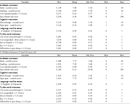
Table 1 tabulates these variables for the two sub samples used by Alaimo et al., 6-11 and

12-16 years old. With respect to the academic and cognitive tests, there is information

about the language used by children to take these tests. The possibilities were English and

Spanish and approximately 96% of the children took the exam in English.

4.2. Food insecurity variable, Hij

The more relevant variable here is “food insecurity”, which is an endogenous variable in

the estimation of school outcome. Therefore, it becomes the dependent variable in the

first step of the estimation (equation (2) above).

The Youth questionnaire asks: “Do you have enough food to eat?”, with the following

alternatives:

1) Enough food to eat

2) Sometimes not enough food to eat

3) Often not enough to eat

8) Blank but applicable

A dummy variable is constructed to distinguish families with or without “food insecurity”

by considering = 1 if the answer is (2) or (3), 0 if answer is (1) and missing value if

answer is (8). In this way, 1,490 families are identified as food-insecure families and they

represent 11% of the total. Table 2 presents the distribution for the full sample and the

two child’s ages sub-samples. Note that this is a family variable, which means that, for

example, if a family has one child between 6-11 years old and another between 12-16

4.3. Family background, FBj

The set of family background variables includes some demographic variables, such as

region of residence and metropolitan area; other variables that characterize the family:

family size, number of family moves (an increasing number of family moves may

negatively affect the child), family head education, employment and marital status,

family income during the previous 12 months to the interview, family income the last

month, the poverty income ratio, and health insurance coverage and its source.

The expected relationships are as follows. Family size affects negatively both school

outcome and food availability, given a certain income level. An increasing number of

family moves is a sign of instability that may affect the children negatively. The years of

education of the family head, as well as his/her employment status (dummy that takes

value 1 if employed in the previous two weeks to the interview) and his/her marital status

(dummy that takes value 1 if married and spouse is present), are expected to positively

affect the dependent variables under study.

The information regarding income is one of the major weaknesses of this survey. There is

no information about actual income. Only some information about income ranges is

available and the rate of non-response is significant. The variable that reports the family

income during the previous 12 months to the interview is divided into categories that start

with “less than 1,000”, increases with interval of a thousand dollars until 20,000 and then

intervals of 5,000 until 50,000 and it is truncated at that point. The variable that reports

the family income during the last month is divided into categories that start with “less

than 100”, increases with interval of a hundred dollars until 1,500 and then intervals of

300 until 4,000 and it is truncated at that point. The variables reported here input to each

family the average income of its correspondent category. Finally, the poverty income

ratio is a ratio between the median income of each category income and a poverty

threshold (the smaller the ratio, the poorer the family). This variable may be useful here

because this is the variable used to determine the eligibility to receive welfare benefits of

Some information about health insurance coverage and its source is also considered. The

alternative sources include Medicare, Medicaid, and others (all kinds of health insurance

plans except those that pay only for accidents).

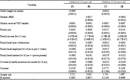
4.4. Individual characteristics, Iij

The individual characteristics set contains variables such as sex, age, weight, and

race-ethnicity, the number of months that receive WIC benefits, low birth weight, mother’s

age at child’s birth, prenatal smoke exposure, and birth complications (the last four are

available only for 6-11 children), variables that may vary within family. Note that here

“mother’s age at child’s birth” is not trying to measure a low income status behavior. In

that case, the relevant variable would be “mother’s age at first birth”, which is trying to

capture the particular impact of mother’s age during pregnancy and birth of each child (so

either very young or very old mothers may put on risk baby’s health).

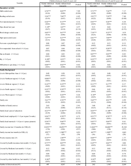
Tables 3 and 4 present means and standard errors for all these variables. They are

tabulated for each family category in terms of food insecurity, including a two-tail mean

difference test. The results are similar for both age groups.

Academic and cognitive outcomes are significatively different between food-insecure and

food-secure families, with the exception of days absent from school for the older group of

children. The psychosocial outcomes present some differences. While younger children

have significant differences with respect to shyness and difficulties to get along with

other children, older ones have significant difference regarding suspension from school

and lack of friends.

Regarding the set of family background characteristics, there are no differences in the

proportion of children living in a metropolitan area. Half of children between 6-11 years

old live in a metropolitan area and almost half (47%) of older children also live in a

metropolitan area.7 There are also no differences in the number of family’s moves for both groups.

All the other variables are significatively different between the two groups. In particular,

families with food insecurity tend to have larger family size; to have a family head less

educated, without employment (in the two weeks before the interview) and not married;

to lack of health insurance and to be poorer.

Surprisingly, the number of families covered by Medicare or Medicaid is not

significatively different between food-insecure and food-secure families in both age

groups.

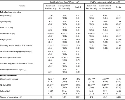
Finally it is the set of individual characteristics. There are no significant differences in

terms of sex, age or weight of children in both groups. With respect to the race-ethnicity

variables, the proportion of black children is not significatively different between families

with or without food insecurity. But there is a significant difference for Hispanic

children: within food-insecure families, 55% (49%) of children between 6 and 11 (12 and

16) years old are Hispanic, against 27% (31%) for food-secure families.

Children in food-insecure families tend to receive the WIC benefits for a longer period

than the ones in food-secure families.

For children between 6 and 11 years old, there are no significative differences for the

dummies of low birth weight and birth complications. Instead, the proportion of mothers

who smoked while pregnant is smaller among food-insecure families, at a significance

level of 10%. In this group, mothers were much younger at their child’s births: 28 against

41 years old. This result might be more associated with the low-income hypothesis of

fertility, which states that poorer people tend to have children at younger stages.

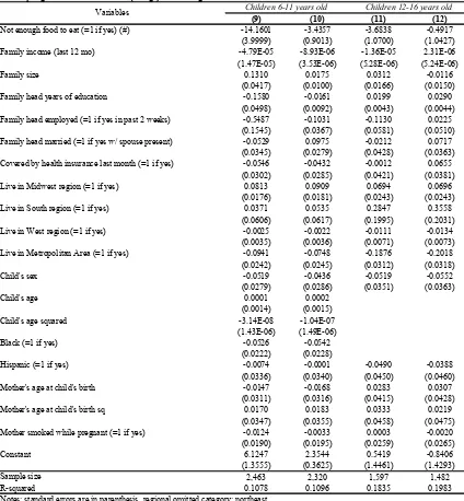
4.5. Are there “good instruments” for food-insecurity?

The key point to prove the causal relationship from nutrition to school outcomes is to

overcome econometric difficulties, due to endogeneity (reverse causality) and omitted

variable (confounding) bias.

In terms of the results, the power of the model relies on its capability to isolate the effect

of nutrition on school outcomes. For example, consider the case in which a child with

of school attendance. One possible interpretation of this observed pattern is that poor

health is the cause of higher absenteeism for this child. But a second plausible

explanation is that the child comes from households with unobservable lower

socioeconomic status, and that this fact leads both to worse educational outcomes and

health outcomes, or similarly, the child has parents with unobservable less interest in both

their child’s health and education, leading to a correlation between child health and

education that is not causal. In many cases it is almost impossible to distinguish between

these two explanations, especially when the data used in the analysis consists of a single

cross-section of observations, as the NHANES III is. One may ask why to work with this

data set. The answer is that the NHANES III is the only source of both health and school

outcome information about children at a national level (and public access).

The variable used to construct the dummy of food-insecurity condition does not vary

within families. This eliminates the use of siblings to control for family fixed effects.

Many of the family background variables influence food-insecurity as well as school

outcomes, such as family income, family head education, employment and marital status,

among others.

At the moment, it is not possible to say that there is a good instrument for food insecurity.

At first sight, the following two instruments appear as potentially reasonable.

First, child’s height. There is a well known positive correlation between nutrition status

and individual’s height. The data used here supports this fact: table 4 reports that children

in food-secure families are significatively taller than the other ones. Disregarding this

fact, there is no reason to expect correlation between height and school outcome.

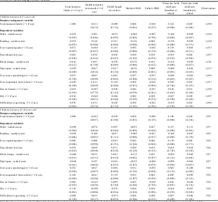
Unfortunately, as table 5 shows, for children between 6-11 years old the only dependent

variable not significatively correlated with height is the digit span score; while for the

older group reading scores and grade repetition are the ones uncorrelated with height.

Second, the body mass index of parents. This variable might be correlated with food

insecurity and uncorrelated with children’s school outcomes. From the data available in

the NHANES it is possible to construct a BMI index for parents. In fact, this variable is

already computed for all surveyed individuals, but it is not possible to find the

mother and father’s weight and height and they can be used to compute the BMI in the

following way:8

(

)

weight (in kg) BMI

height (in cm) 100

= .

Table 4 presents the statistics for mother and father’s BMI. In both age groups the

average mother’s BMI is higher for families with food insecurity, while the average

father’s BMI index is not significatively different between the two groups. One possible

explanation of the higher average BMI among mothers with food-insecurity condition is

that there might be a higher proportion of obese mothers, which can be considered as a

sign of low quality food.9

The correlation of mother’s BMI and food-insecurity is very strong, as can be seen in

Table 5. Regrettable, it is also correlated, at a 10% significance level with the whole set

of dependent variables. On the contrary, father’s BMI appears to have no relation not

only with school outcome variables but also with the food-insecurity one.

These results suggest that none of them can be considered as “good” instruments for food

insecurity. Next section presents some regressions using these “bad instruments”.

Although the results appear to be good, it is not possible to draw conclusions from it, as

the ones presented in Alaimo et al. (2001). Finally, the last section includes other

potentially plausible instrument that might be constructed using the NHANES and that

will be subject of future research.

8

This formula is the one used by NHANES to compute the variable BMI and it is based in centimeters and kilograms. The variables for mother and father’s height and weight are expressed in inches and pounds, so will convert them using the following scale: 1 inch = 2.54 cm, 1 pound = .4536 kg

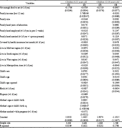
5. Empirical results using “bad” instruments

At this stage of the analysis, it seems that the NHANES III does not contain information

to find empirical evidence of a causal relationship between food-insecurity and school

outcomes. For the sake of simplicity, this section only includes results for one dependent

variable, “math scaled scores”. Although there are variations using different dependent

variables, the point here is to address the quality of the instruments, which is similar with

respect to the reminding dependent variables.

First, it might be interesting to see the simple OLS estimation of school outcomes on

food-insecurity. Table 6 reports a significant relationship between these variables; even

controlling for some family and individual characteristics, this relationship remains

significatively different from zero. But it has been argued here that these estimations

cannot be interpreted as a causal relationship because of the presence of unobservables

that affect both food-insecurity and school outcome. The problem does not end up there.

It is necessary to find a good instrument to eliminate this endogeneity problem.

The first step is to estimate equation (2), which has a binary variable as dependent

variable. Table 7 presents the results based on a linear probability model for

food-insecurity. Two of the instruments presented in section 4.5 (child’s height and mother’s

BMI) are used alternatively as explanatory variables for the two age sub-samples. The

results indicate that these variables are not good enough in explaining families’

food-insecurity. Only in model (6), where mother’s BMI is used to instrument food-insecurity

among children of 6 to 11 years old, this variable turns to be significatively different from

zero. But as seen in the correlation table, it is not exogenous with respect to school

outcome.

However, when using these estimates in the second step (equation (1) of the theoretical

model), Table 8 shows that there is a strong and negatively significant relationship

between food insecurity and school outcomes (in particular, math scores).

This is the source of criticism to many nutritional studies as the one of Alaimo et al

(2001). In spite of the efforts made in order to control for unobserved characteristics that

variable bias-, the present study shows that with the tools provided by NHANES III it is

not possible to identify a good instrument to account for these empirical problems.

6. Conclusions and future research

Is it possible to show a causal relationship between nutrition and education using

cross-section data? At the moment, the answer is “NO”.

Although the empirical results can be viewed by a careless reader as evidence in favor of

this relationship, they are still subject to endogeneity and omitted variable bias and

therefore inferences cannot be made. This is not only true for this study, but also for the

results of Alaimo et al. (among others) that face the same limitations as the ones detailed

here.

At this point, there are two alternatives. One is to consider that these results are enough

evidence to conclude that this empirical strategy is inappropriate and should be avoided.

The other is to keep on trying to check if there are any other variables in the survey that

can be used to overcome these identification problems. Given that there are no many

other ways to study this link, at least, using public data sets with national representation,

it might be worth while to insist in this path of work.

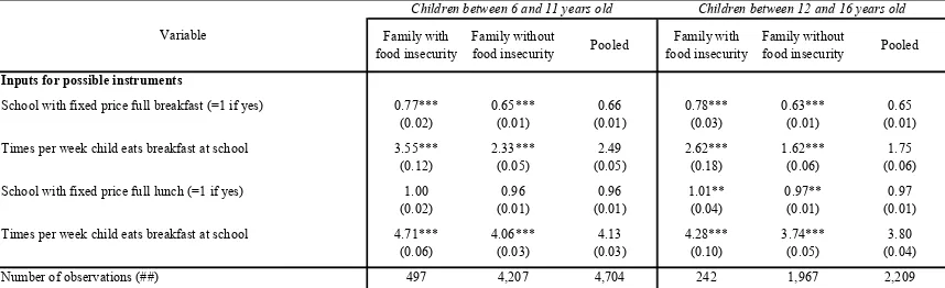
In fact, there are already identified other instruments which can be developed.

One possibility would be to construct an exogenous state policy variable that relates the

availability of different levels of food assistance at school with the use of these programs

by children from food-insecure families. The construction of this variable would take

some steps.

First, the NHANES III contains some information about state of residence: there is a

variable that indicate the state of residence if the family lives in a county with a

population of more than 500,000 habitants. Therefore, one might narrow the analysis to

children living in metropolitan areas. Second, there is also information about breakfast

and lunch served at school at a fixed price, and also the frequency (days per week) that

four variables –and the results show that there is a significative difference in the use of

these programs between food-secure and food-insecure children. Third, the survey was

conducted between 1988 and 1994. Although there is no information about the exact

moment at which each interview took place, there are some phases and sub-phases of

data collection. Fourth, it would be necessary to collect from other sources the existence

of state school breakfast and lunch programs, their coverage and their year of

implementation (and further extensions). Combining all these variables it could be

possible to find variation between states and within states for different periods.

Another possibility is the use of the poverty-income ratio to determine the eligibility of

families to programs such as the WIC. Together with other eligibility criteria, this

information could be use to construct a variable that accounts for the availability and

effective use of this kind of public programs.

If after these and other attempts is still unattainable to find a good instrument for

food-insecurity, i.e., if this “good instrument” does not exist, the results of this study would

imply that it is not possible to use cross-section data sets, in particular, the NHANES III,

References

Alaimo, K., Olson, C., and Fronguillo, E. (2001) “Food Insufficiency and American

School- Aged Children's Cognitive, Academic, and Psychosocial Development”

Pediatrics, 108(1), 44-53.

Behrman, J., Rosenzweig, M., Taubman, P. (1994) “Endowments and the Allocation of

Schooling in the Family and in the Marriage Market: The Twins Experiment”, Journal of

Political Economy, 102(6), 1131-1174.

Card, D. (1999) "The Causal Effect of Education on Earnings," Handbook of Labor

Economics, 3a, Chapter 30.

Case, A., Lubotsky, D. and Paxton, C. (2002) “Economic Status and Health in

Childhood: The Origins of the Gradient”, American Economic Review, 92(5).

Figlio, D. and Winicki, J. (2002) “Food for Thought: the Effects of School

Accountability Plans on School Nutrition”, NBER Working Paper 9319

Heckman, J. (1978) “Dummy Endogenous Variables in a Simultaneous Equation

System”, Econometrica, 46(4), 931-959.

Heckman, J., and Macurdy, T., (1986) “Labor Econometrics”, Handbook of

Econometrics, III, Chapter 32.

Hicks, Langham, and Takenaka (1982) “Cognitive and Health Measures Following Early

Nutritional Supplementation: a Siblings Study”, American Journal of Public Health,

72(10).

Horrace, W. and Oaxaca, R. (2003) “New Wine in Old Bottles: A Sequential Estimation

Technique for the LPM”

Kennedy, E. and Davis, C. (1998) “US Department of Agriculture School Breakfast

Program”, American Journal of Clinical Nutrition, 67(suppl.), 798S-803S

Miguel, E. (2003) “Health, Education and Economic Development”, Chapter 15 of a

forthcoming book of MIT press.

Miguel, E. and Kramer, M. (2003) “Worms: Identifying Impacts on Education and Health

Pollit, E., Gorman, K.S., Engle, P., Martorell, R. and Rivera, J.A. (1993) “Early

Supplementary Feeding and Cognition: Effects Over Two Decades”, Monographs of the

Society for Research in Child Development, 58(7).

Strauss, J. and Thomas, D. (1998) “Health, Nutrition, and Economic Development”,

Journal of Economic Literature, 36, 766-817.

U.S. Department of Health and Human Services (DHHS), National Center for Health

Statistics, Third National Health and Nutrition Examination Survey, 1988-1994,

NHANES III Examination Data File, Examination Documentation File, Youth Data File

Table 1

Descriptive statistic of the dependent variable: school outcomes, 1988-1994 I. Children between 6 and 11 years old

Variable Obs Mean Std. Dev. Min Max

Academic outcomes

Math - scaled scores 3,139 7.89 3.34 0 20

Reading - scaled scores 3,129 6.85 3.78 0 18

Ever repeated grade (=1 if yes) 3,317 0.16 0.37 0 1

Days absent last year 3,434 4.56 7.99 0 240

Cognitive outcomes

Block design - scaled score 3,119 8.60 3.34 1 19

Digit span - scaled score 3,116 8.16 3.00 1 19

Language used in exams

1 if English, 0 if Spanish 3,134 0.95 0.21 0 1

Psychosocial outcomes

Ever seen a psychologist (=1 if yes) 3,461 0.07 0.26 0 1 Ever suspended from school (=1 if yes) 3,318 0.04 0.21 0 1

Has no friends (=1 if yes) 4,720 0.03 0.17 0 1

Shy (=1 if yes) 3,461 0.24 0.42 0 1

Difficulties to get along (=1 if yes) 3,461 0.02 0.15 0 1

II. Children between 12 and 16 years old

Variable Obs Mean Std. Dev. Min Max

Academic outcomes

Math - scaled scores 1,940 7.17 3.40 0 20

Reading - scaled scores 1,931 7.39 3.60 0 17

Ever repeated grade (=1 if yes) 2,210 0.28 0.45 0 1

Days absent last year 2,182 8.12 24.81 0 365

Cognitive outcomes

Block design - scaled score 1,915 8.19 3.41 1 19

Digit span - scaled score 1,915 7.72 2.85 1 19

Language used in exams

1 if English, 0 if Spanish 1,939 0.97 0.18 0 1

Psychosocial outcomes

Ever seen a psychologist (=1 if yes) 2,211 0.13 0.34 0 1

Ever suspended (=1 if yes) 2,210 0.21 0.41 0 1

Has no friends (=1 if yes) 2,216 0.03 0.18 0 1

Shy (=1 if yes) 2,213 0.23 0.42 0 1

Difficulties to get along (=1 if yes) 2,212 0.02 0.15 0 1

Source: NHANES III Exam Data and Documentation Files

Note: Cognitive function was evaluated using parts of two tests, the Wechsler Intelligence Scale for Children-Revised (WISC-R) and the Wide Range Achievement Test-Revised (WRAT-R). Two subtests of the WISC-R test, a verbal component (Digit Span) and a performance exam (Block Design), were administered and are considered relatively culturally unbiased (Kaufman, 1979). In addition, two subtests of the WRAT-R test, math and reading, were conducted. The WISC-R test was administered first and was followed by the WRAT-R. The scores for all four subtests used a common scale and were derived for each child relative to his/her age group based on test-specific standardization samples created by the test developers (Wechsler, 1974; Jastak, 1984; Kramer, 1995).

Table 2

Families and food insecurity: Do you have enough food to eat?

Obs % Obs % Obs %

Yes 12,407 89.28 4,207 89.43 1,967 89.04

No 1,490 10.72 497 10.57 242 10.96

Total 13,897 100.00 4,704 100.00 2,209 100.00

Source: NHANES III Youth Data File

I. Full Sample II. Children 6-11 III. Children 12-16

Family with food insecurity

Family without food insecurity Pooled

Family with food insecurity

Family without food insecurity Pooled

Dependent variable

Math scaled score 6.76*** 8.03*** 7.89 5.71*** 7.36*** 7.17 (0.16) (0.06) (0.06) (0.20) (0.08) (0.08) Reading scaled score 5.36*** 7.04*** 6.85 5.91*** 7.59*** 7.40

(0.19) (0.07) (0.07) (0.22) (0.09) (0.08) Ever repeated grade (=1 if yes) 0.26*** 0.15*** 0.16 0.43*** 0.26*** 0.28

(0.02) (0.01) (0.01) (0.03) (0.01) (0.01) Days absent last year 5.34** 4.47** 4.57 9.15 8.02 8.14

(0.47) (0.14) (0.14) (0.91) (0.59) (0.53) Block design scaled score 8.05*** 8.67*** 8.60 7.18*** 8.32*** 8.19

(0.16) (0.06) (0.06) (0.23) (0.08) (0.08) Digit span scaled score 7.27*** 8.27*** 8.16 6.81*** 7.84*** 7.72

(0.15) (0.06) (0.05) (0.20) (0.07) (0.07) Ever seen a psychologist (=1 if yes) 0.08 0.07 0.07 0.15 0.13 0.13

(0.01) (0.00) (0.00) (0.02) (0.01) (0.01) Ever suspended from school (=1 if yes) 0.07 0.04 0.04 0.34*** 0.20*** 0.22

(0.01) (0.00) (0.00) (0.03) (0.01) (0.01) Has no friends (=1 if yes) 0.04 0.03 0.03 0.07*** 0.03*** 0.03

(0.01) (0.00) (0.00) (0.02) (0.00) (0.00) Shy (=1 if yes) 0.28** 0.23** 0.24 0.32*** 0.22*** 0.23

(0.02) (0.01) (0.01) (0.03) (0.01) (0.01) Difficulties to get along (=1 if yes) 0.04*** 0.02*** 0.02 0.03 0.02 0.02

(0.01) (0.00) (0.00) (0.01) (0.00) (0.00)

Family Background

Live in Metropolitan Area (=1 if yes) 0.49 0.50 0.50 0.43 0.48 0.47 (0.02) (0.01) (0.01) (0.03) (0.01) (0.01) Live in Northeast region (=1 if yes) 0.085** 0.12** 0.11 0.12 0.11 0.11

(0.01) (0.00) (0.00) (0.02) (0.01) (0.01) Live in Midwest region (=1 if yes) 0.14*** 0.19*** 0.19 0.11*** 0.17*** 0.17

(0.02) (0.01) (0.01) (0.02) (0.01) (0.01) Live in South region (=1 if yes) 0.32*** 0.39*** 0.39 0.46 0.42 0.42

(0.02) (0.01) (0.01) (0.03) (0.01) (0.01) Live in West region (=1 if yes) 0.42*** 0.24*** 0.26 0.30** 0.24** 0.01

(0.02) (0.01) (0.01) (0.03) (0.01) (0.43) Family size 5.61*** 4.76*** 4.85 5.62*** 4.91*** 4.99

(0.10) (0.03) (0.03) (0.13) (0.04) (0.04) Number of family moves 2.62 2.96 2.91 3.40 3.48 3.47

(0.14) (0.08) (0.07) (0.23) (0.11) (0.10) Family head years of education 8.21*** 11.48*** 11.14 8.65*** 11.08*** 10.82 (0.19) (0.06) (0.06) (0.26) (0.09) (0.08) Family head employed (=1 if yes in past 2 weeks) 0.56*** 0.78*** 0.75 0.51*** 0.78*** 0.75

(0.02) (0.01) (0.01) (0.03) (0.01) (0.01) Family head married (=1 if yes w/ spouse present) 0.54*** 0.68*** 0.66 0.43*** 0.64*** 0.61

(0.02) (0.01) (0.01) (0.03) (0.01) (0.01) Family income last 12 months (in US$) (#) 12,055*** 26,093*** 24,682 11,064*** 26,880*** 25,242 (374) (250) (237) (500) (376) (357) Family income last month (in US$) (#) 878*** 1,940*** 1,831 847*** 1,989*** 1,865 (27) (20) (19) (36) (30) (28) Poverty income ratio (#) 0.75*** 1.89*** 1.77 0.69*** 1.89*** 1.77 (0.03) (0.02) (0.02) (0.03) (0.03) (0.03) Covered by health insurance last month (=1 if yes) 0.77*** 0.87*** 0.86 0.67*** 0.82*** 0.80

(0.02) (0.01) (0.01) (0.03) (0.01) (0.01) Covered by Medicare last month (=1 if yes) 0.13 0.06 0.07 0.13 0.05 0.05

(0.07) (0.02) (0.02) (0.13) (0.02) (0.02) Covered by Medicaid last month (=1 if yes) 0.89 0.86 0.87 0.69 0.76 0.74

(0.02) (0.01) (0.01) (0.04) (0.02) (0.02) Covered by other health ins. last month (=1 if yes) 0.86** 0.92** 0.91 0.82** 0.90** 0.90

(0.03) (0.01) (0.01) (0.05) (0.01) (0.01) Number of observations (##) 497 4,207 4,704 242 1,967 2,209

Source: NHANES III Youth and Exam data files

Descriptive statistic of dependent and family background variables, clasiffied according to "family food insecurity" Table 3

Note: Standard errors are in parenthesis. * indicates a statistically significant difference between food-insecure and food-secure families at a 90% confidence interval, ** at a 95% and *** at a 99% confidence interval. (#) Income variables are reported in categories. Here it was attached to each variable the mean income of each category. The poverty income ratio is a ratio between the median income of each category income and a poverty threshold, i.e., the smaller the ratio, the poorer the family. This variable is subject to nonresponse error. See footnote in text. (##) The total number of observations for each variable may vary due to missing cases.

Children between 12 and 16 years old Variable

Family with food insecurity

Family without

food insecurity Pooled

Family with food insecurity

Family without

food insecurity Pooled

Individual characteristics

Sex (=1 if boy) 0.49 0.51 0.51 0.48 0.47 0.47

(0.02) (0.01) (0.01) (0.03) (0.01) (0.01)

Age (in years) 8.55 8.51 8.51 13.98 13.99 13.98

(0.08) (0.03) (0.03) (0.09) (0.03) (0.03)

Black (=1 if yes) 0.28 0.29 0.29 0.38 0.36 0.36

(0.02) (0.01) (0.01) (0.03) (0.01) (0.01)

Hispanic (=1 if yes) 0.55*** 0.27*** 0.30 0.49*** 0.31*** 0.33

(0.02) (0.01) (0.01) (0.03) (0.01) (0.01)

Weight (in lbs) 60.48 59.00 59.16 127.63 129.96 129.69

(1.46) (0.51) (0.48) (2.29) (0.82) (0.77)

How many months received WIC benefits 17.29*** 17.28*** 17.28 27.71 25.68 25.91

(0.65) (0.25) (0.23) (1.28) (0.44) (0.42)

Mother smoked while pregnant (=1 if yes) 0.17* 0.21* 0.21

(0.02) (0.01) (0.01)

Mother's age at child's birth 28.10** 40.96** 39.60

(2.63) (1.87) (1.70)

Low birth weight (= 1 if less than 5 1/2 lbs) 0.09 0.07 0.07

(0.01) (0.00) (0.00)

Birth complications (=1 if yes) (2) 0.12 0.11 0.11

(0.01) (0.00) (0.00)

Possible instruments?

Child's height (in inches) 52.52* 52.97* 52.92 63.31*** 64.01*** 63.93

(0.26) (0.09) (0.08) (0.24) (0.09) (0.08)

Mother's BMI 27.25*** 25.60*** 25.76 28.40*** 27.17*** 27.29

(0.29) (0.09) (0.09) (0.46) (0.15) (0.14)

Father's BMI 26.15 26.36 26.34 26.91 26.93 26.93

(0.22) (0.07) (0.07) (0.37) (0.11) (0.11)

Number of observations (##) 497 4,207 4,704 242 1,967 2,209

Source: NHANES III Youth and Exam data files

Descriptive statistic for individual characteristics and possible instrument variables, clasiffied according to "family food insecurity" Table 4

Note: Standard errors are in parenthesis. * indicates a statistically significant difference between food-insecure and food-secure families at a 90% confidence interval, ** at a 95% and *** at a 99% confidence interval

(##) The total number of observations for each variable may vary due to missing cases

Children between 12 and 16 years old

Variable

Table 5

Partial correlation among relevant variables

Food-insecure family (=1 if yes)

Health insurance last month (=1 if

yes)

Child's height

(in inches) Mother's BMI Father's BMI

Times per week child eats breakfast at

school

Times per week child eats breakfast at

school

Observations

Children between 6-11 years old

Dummy endogenous variable

Food-insecure family (=1 if yes) 1.000 -0.011 -0.009 0.088 -0.030 0.163 0.029 1,498 (0.672) (0.716) (0.001) (0.253) (0.000) (0.268)

Dependent variables

Math - scaled scores -0.051 0.053 0.074 -0.084 -0.007 -0.160 -0.004 1,428

(0.055) (0.046) (0.005) (0.002) (0.798) (0.000) (0.887)

Reading - scaled scores -0.051 0.120 0.267 -0.126 0.005 -0.210 -0.029 1,420

(0.053) (0.000) (0.000) (0.000) (0.844) (0.000) (0.271)

Ever repeated grade (=1 if yes) 0.071 -0.044 0.101 0.093 -0.036 0.119 -0.003 1,451 (0.007) (0.097) (0.000) (0.000) (0.170) (0.000) (0.911)

Days absent last year 0.003 0.058 -0.052 0.034 0.018 -0.015 0.002 1,497

(0.899) (0.025) (0.047) (0.192) (0.478) (0.552) (0.930)

Block design - scaled score 0.014 0.007 -0.070 -0.070 0.013 -0.214 -0.059 1,416

(0.611) (0.798) (0.009) (0.008) (0.632) (0.000) (0.027)

Digit span - scaled score -0.052 0.067 0.027 -0.076 0.004 -0.090 -0.028 1,417

(0.049) (0.012) (0.320) (0.005) (0.891) (0.001) (0.301)

Ever seen a psychologist (=1 if yes) 0.037 0.043 0.082 0.017 -0.017 -0.048 -0.001 1,496 (0.158) (0.099) (0.002) (0.506) (0.518) (0.063) (0.967)

Ever suspended from school (=1 if yes) 0.030 0.011 0.108 0.002 -0.018 0.038 0.025 1,451 (0.260) (0.669) (0.000) (0.951) (0.494) (0.146) (0.347)

Has no friends (=1 if yes) -0.027 -0.007 -0.039 0.046 -0.033 0.018 0.033 1,498

(0.303) (0.775) (0.132) (0.078) (0.201) (0.485) (0.203)

Shy (=1 if yes) 0.014 -0.060 -0.006 0.002 0.028 -0.027 0.029 1,497

(0.586) (0.021) (0.806) (0.925) (0.274) (0.290) (0.269)

Difficulties to get along (=1 if yes) 0.078 0.031 -0.025 0.038 -0.022 -0.015 0.022 1,498 (0.003) (0.234) (0.332) (0.143) (0.396) (0.559) (0.395)

Children between 12-16 years old

Dummy endogenous variable

Food-insecure family (=1 if yes) 1.000 -0.062 -0.034 0.024 -0.048 0.148 0.030 950 (0.057) (0.300) (0.453) (0.139) (0.000) (0.356)

Dependent variables

Math - scaled scores -0.095 0.076 0.095 -0.093 0.027 -0.137 -0.111 897

(0.004) (0.024) (0.004) (0.005) (0.430) (0.000) (0.001)

Reading - scaled scores -0.093 0.108 0.051 -0.089 -0.021 -0.188 -0.047 889

(0.006) (0.001) (0.131) (0.008) (0.527) (0.000) (0.159)

Ever repeated grade (=1 if yes) 0.086 0.000 0.043 0.045 0.006 0.134 0.045 950

(0.008) (0.998) (0.191) (0.164) (0.864) (0.000) (0.171)

Days absent last year 0.074 0.004 0.071 0.050 0.032 -0.012 -0.034 946

(0.023) (0.908) (0.030) (0.129) (0.335) (0.725) (0.292)

Block design - scaled score -0.086 0.033 0.083 -0.115 0.023 -0.050 -0.068 887

(0.011) (0.331) (0.014) (0.001) (0.507) (0.141) (0.044)

Digit span - scaled score -0.064 0.107 0.066 -0.055 -0.060 -0.099 -0.062 887

(0.061) (0.002) (0.053) (0.107) (0.078) (0.004) (0.067) Ever seen a psychologist (=1 if yes) 0.072 0.027 0.086 0.011 -0.074 -0.041 -0.100 948

(0.028) (0.407) (0.009) (0.736) (0.024) (0.212) (0.002) Ever suspended from school (=1 if yes) 0.102 0.041 0.159 0.053 0.002 0.085 -0.050 950

(0.002) (0.206) (0.000) (0.107) (0.958) (0.009) (0.123)

Has no friends (=1 if yes) 0.003 -0.025 0.009 0.035 -0.010 0.056 -0.044 950

(0.925) (0.450) (0.784) (0.284) (0.759) (0.087) (0.176)

Shy (=1 if yes) 0.110 -0.090 -0.072 0.030 0.054 -0.034 -0.007 950

(0.001) (0.006) (0.026) (0.364) (0.096) (0.293) (0.838) Difficulties to get along (=1 if yes) 0.050 0.033 -0.073 0.028 0.040 -0.027 -0.046 950

(0.129) (0.317) (0.025) (0.396) (0.215) (0.409) (0.156) Source: NHANES III Youth and Exam data files

Table 6

OLS regression on math scores (in logs)

(1) (2) (3) (4)

Not enough food to eat (=1 if yes) -0.1786 -0.0739 -0.2519 -0.0987 (0.0264) (0.0304) (0.0376) (0.0377)

Family income (last 12 mo) 3.76E-06 -0.0201

(8.02E-07) (0.0069)

Family size -0.0146 0.0302

(0.0058) (0.0038)

Family head years of education 0.0170 0.0692

(0.0031) (0.0299) Family head employed (=1 if yes in past 2 weeks) -0.0118 0.1247

(0.0247) (0.0267) Family head married (=1 if yes w/ spouse present) 0.0371 0.1219

(0.0229) (0.0307) Covered by health insurance last month (=1 if yes) -0.0010 0.0476

(0.0263) (0.0232)

Live in Midwest region (=1 if yes) -0.0074 -0.0281

(0.0336) (0.0440)

Live in South region (=1 if yes) -0.0199 0.0304

(0.0312) (0.0406)

Live in West region (=1 if yes) 0.0165 0.0471

(0.0347) (0.0447)

Live in Metropolitan Area (=1 if yes) -0.0120 -0.0048

(0.0190) (0.0252)

Child's sex 0.0793 0.3852

(0.0177) (0.1932)

Child's age 0.0561 -0.0144

(0.0604) (0.0069)

Child's age squared -0.0024 -0.1964

(0.0035) (0.0304)

Black (=1 if yes) -0.0837 -0.0634

(0.0241) (0.0344)

Hispanic (=1 if yes) -0.0499

(0.0279)

Mother's age at child's birth 0.0005

(0.0014) Mother's age at child's birth sq -3.98E-07

(1.43E-06) Mother smoked while pregnant (=1 if yes) -0.0572

(0.0222)

Constant 2.0322 1.4485 1.9074 -1.1015

(0.0089) (0.2620) (0.0127) (1.3437)

Sample size 3,029 2,468 1,889 1,599

R-squared 0.0149 0.1021 0.0232 0.1798

Notes: standard errors are in parenthesis, regional omitted category: northeast

Table 7

First step LPM estimation: food-insecurity dummy

(5) (6) (7) (8)

Child's height (in inches) -0.0007 -0.0022

(0.0012) (0.0019)

Mother's BMI 0.0017 -0.0002

(0.0008) (0.0012) Months received WIC benefits 0.0001 0.0001 0.0005 0.0007

(0.0004) (0.0003) (0.0004) (0.0004)

Family size 0.0103 0.0088 0.0137 0.0124

(0.0036) (0.0030) (0.0042) (0.0044) Family income (last 12 mo) -3.67E-06 -3.77E-06 -4.79E-06 -4.88E-06

(4.85E-07) (3.96E-07) (5.95E-07) (6.17E-07) Family head years of education -0.0124 -0.0095 -0.0013 -0.0005

(0.0018) (0.0016) (0.0023) (0.0025) Family head employed (=1 if yes in past 2 weeks) -0.0380 -0.0267 -0.0455 -0.0385 (0.0154) (0.0128) (0.0192) (0.0198) Family head married (=1 if yes w/ spouse present) -0.0065 0.0161 -0.0279 -0.0182 (0.0140) (0.0116) (0.0173) (0.0178) Covered by health insurance last month (=1 if yes) -0.0036 -0.0098 -0.0254 -0.0164 (0.0164) (0.0148) (0.0195) (0.0206)

Constant 0.3529 0.2269 0.3775 0.2194

(0.0684) (0.0358) (0.1268) (0.0530)

Sample size 2,721 3,482 1,741 1,607

R-squared 0.1091 0.0955 0.1104 0.0989

Notes: standard errors are in parenthesis Variables

Table 8

2nd step regression on math scores (in logs) - not enough food to eat instrumented

(9) (10) (11) (12)

Not enough food to eat (=1 if yes) (#) -14.1601 -3.4357 -3.6838 -0.4917 (3.9999) (0.9013) (1.0700) (1.0427) Family income (last 12 mo) -4.79E-05 -8.93E-06 -1.36E-05 2.31E-06 (1.47E-05) (3.53E-06) (5.28E-06) (5.24E-06)

Family size 0.1310 0.0175 0.0312 -0.0116

(0.0417) (0.0100) (0.0166) (0.0150) Family head years of education -0.1580 -0.0161 0.0199 0.0290

(0.0498) (0.0092) (0.0043) (0.0044) Family head employed (=1 if yes in past 2 weeks) -0.5487 -0.1031 -0.1130 0.0225

(0.1545) (0.0367) (0.0581) (0.0510) Family head married (=1 if yes w/ spouse present) -0.0529 0.0975 -0.0212 0.0717

(0.0345) (0.0279) (0.0428) (0.0363) Covered by health insurance last month (=1 if yes) -0.0546 -0.0432 -0.0012 0.0655

(0.0302) (0.0285) (0.0421) (0.0381) Live in Midwest region (=1 if yes) 0.0813 0.0909 0.0694 0.0696

(0.0176) (0.0181) (0.0243) (0.0243) Live in South region (=1 if yes) 0.0371 0.0535 0.2847 0.3558

(0.0606) (0.0617) (0.1995) (0.2031) Live in West region (=1 if yes) -0.0025 -0.0022 -0.0111 -0.0134 (0.0035) (0.0036) (0.0071) (0.0073) Live in Metropolitan Area (=1 if yes) -0.0941 -0.0748 -0.1876 -0.2018 (0.0242) (0.0245) (0.0312) (0.0318)

Child's sex -0.0519 -0.0436 -0.0519 -0.0552

(0.0279) (0.0286) (0.0351) (0.0363)

Child's age 0.0001 0.0002

(0.0014) (0.0015) Child's age squared -3.14E-08 -1.04E-07

(1.43E-06) (1.49E-06)

Black (=1 if yes) -0.0526 -0.0542

(0.0222) (0.0228)

Hispanic (=1 if yes) -0.0074 -0.0001 -0.0490 -0.0388

(0.0336) (0.0340) (0.0450) (0.0460) Mother's age at child's birth -0.0147 -0.0168 0.0283 0.0307

(0.0311) (0.0316) (0.0415) (0.0428) Mother's age at child's birth sq 0.0170 0.0183 0.0333 0.0219

(0.0347) (0.0355) (0.0458) (0.0475) Mother smoked while pregnant (=1 if yes) -0.0124 -0.0033 0.0003 -0.0020 (0.0190) (0.0195) (0.0259) (0.0265)

Constant 6.1247 2.3544 0.5419 -0.8406

(1.3555) (0.3625) (1.4461) (1.4293)

Sample size 2,463 2,320 1,597 1,482

R-squared 0.1078 0.1096 0.1835 0.1983

Notes: standard errors are in parenthesis, regional omitted category: northeast

Variables Children 6-11 years old Children 12-16 years old

Family with food insecurity

Family without food insecurity Pooled

Family with food insecurity

Family without food insecurity Pooled

Inputs for possible instruments

School with fixed price full breakfast (=1 if yes) 0.77*** 0.65*** 0.66 0.78*** 0.63*** 0.65

(0.02) (0.01) (0.01) (0.03) (0.01) (0.01)

Times per week child eats breakfast at school 3.55*** 2.33*** 2.49 2.62*** 1.62*** 1.75

(0.12) (0.05) (0.05) (0.18) (0.06) (0.06)

School with fixed price full lunch (=1 if yes) 1.00 0.96 0.96 1.01** 0.97** 0.97

(0.02) (0.01) (0.01) (0.04) (0.01) (0.01)

Times per week child eats breakfast at school 4.71*** 4.06*** 4.13 4.28*** 3.74*** 3.80

(0.06) (0.03) (0.03) (0.10) (0.05) (0.04)

Number of observations (##) 497 4,207 4,704 242 1,967 2,209

Source: NHANES III Youth and Exam data files

Note: Standard errors are in parenthesis. * indicates a statistically significant difference between food-insecure and food-secure families at a 90% confidence interval, ** at a 95% and *** at a 99% confidence interval

(##) The total number of observations for each variable may vary due to missing cases

Descriptive statistic, selected variables, clasiffied according to "family food insecurity" Table 9

Children between 12 and 16 years old

Variable