The short-run dynamics of inflation: estimating a "hybrid new Keynesian Phillips curve" for Argentina

Universidad Nacional de La Plata

Novenas Jornadas de Economía

Monetaria e Internacional

La Plata, 6 y 7 de mayo de 2004

The Short–Run Dynamics of Inflation: Estimating a "Hybrid

New Keynesian Phillips Curve" for Argentina

The Short –run Dynamics of Inflation:

Estimating a “Hybrid New Keynesian Phillips Curve” for Argentina1

Laura D’Amato*

ldamato@bcra.gov.ar

and Lorena Garegnani**

lgaregnani@bcra.gov.ar

Based on recent developments in the empirical modeling of the short-run dynamics of

inflation, we estimate a “Hybrid New Keynesian Phillips Curve” for Argentina over the

period 1993-2003, which assumes that while a fraction of the firms are forward-looking,

the others use a backward-looking rule to set prices. We extend the model to a small

open economy, considering the influence of nominal devaluation and foreign inflation

on domestic prices. Although we find a significant forward-looking behavior,

backwardness seems to be more relevant for domestic prices setting. Finally, we

cannot reject verticality of the Phillips Curve in the long run.

JEL: C5, E31

*BCRA and D. Candidate UNLP.

**BCRA, UNLP and D. Candidate UNLP.

1

1. Introduction

Assessing the short run dynamics of inflation is a relevant issue for monetary policy. A

distinctive feature of recent theoretical developments in modeling inflation in the

short-run is the introduction of some nominal rigidity in the context of inter-temporal

optimizing behavior by non-competitive forward-looking firms. In these models, built on

earlier work by Taylor (1980), Calvo (1983) and Fischer (1997), price stickiness could

arise for different reasons. In Calvo’s (1983) setting some sluggishness in price

formation could be obtained by assuming that forward-looking firms face constraints on

price adjustment. The resulting model is a New Keynesian, forward-looking version of

the traditional Phillips Curve. The empirical relevance of inflation persistence, which

imposes costs for disinflation policies has led to incorporate inflation inertia in these

models, in spite of the theoretical difficulties to justify it. Galí and Gertler (1999) extend

the Calvo’s model, allowing for a portion of the firms to follow a backward-looking rule

to set prices and obtain a “Hybrid New Keynesian Phillips Curve”.

Based on these theoretical grounds, an empirical literature has developed and many

issues related to theoretical and empirical aspects of these models are currently under

debate. Models based on Calvo’s (1983) setting have been subject to the critique of

being quite unrealistic in assuming that firms should not expect to adjust prices in a

finite horizon and it has been suggested that some truncation should be introduced to

add them a quote of realism. The use of the output gap as a measure of marginal costs

has also been questioned for both theoretical and empirical reasons. Galí and Gertler

(1999) suggest using the aggregate labor income share as a a measure of marginal

cost instead of the output gap.

We study here how well the so-called “Hybrid New Keynesian Phillips Curve”

approximates the dynamics of inflation in Argentina over the period 1993-2003. The

standard model is modified to capture the role played by the nominal exchange rate

and foreign prices in domestic prices dynamics in a small open economy. This is a

difficult task in the case of Argentina, because the economy went into structural

changes after the devaluation of the peso that followed the financial and currency

crises of 2001. In this context, it is highly probable that the dynamics of price setting

has changed after the abandonment of the currency board regime and the adoption of

To estimate this New Keynesian version of the Phillips Curve we use the Generalized

Method of Moments (GMM), which seems to be the appropriate method under rational

expectations, since it is based on the assumption that the error in forecasting inflation

by firms is orthogonal to the available information.

The paper is organized as follows: in section 2 we briefly present some recent

theoretical developments in modeling inflation dynamics. Section 3 describes the

estimation methodology. In section 4, we present the empirical results and, finally,

section 5 concludes.

2. Recent developments in modeling inflation dynamics

In the hybrid version of the Phillips Curve proposed by Galí and Gertler (1999) inflation

follows the process

) ( )

( ) 1

( ₁

1 Et t mct t 1

t

t φπ φ π δ ε

π = − + − + + +

Where πt is the inflation rate at time t, Etis the expectation of inflation on t+1 at time t,

mctis the marginal cost and εt is a random shock. The assumption that 0 < φ < 1, implies a vertical Phillips curve in the long run. The lagged term in inflation introduces

some backwardness in price setting, an observable feature of inflation dynamics, which

is quite difficult to justify from a theoretical point of view. In Calvo’s framework, firms

operate in a monopolistically competitive environment and face some constraints in

prices setting in the form of a time dependent rule of adjustment. More specifically each

firm faces a constant probability (1-θ) of adjusting prices in period t and a corresponding constant probability θ of maintaining its prices unchanged.

This implies that the price level in t is a convex combination of prices optimally set in previous periods p_t−j and prices optimally set in t p*_t according to

) 2 ( p ) 1 ( p p

) 1 (

p *

t 1

t j t *

0 j

j

t = −θ θ − =θ − + −θ

∞

=

∑

{ }

) ( ) 1 (

p _{t t j}

0 j

j *

t +

∞

=

∑

Which assumes that firms are identical and choose the same p*_t according to their

expected marginal costs for future periods mct+j , discounted at the subjective factor β.

Combining (2) and (3) an inflation equation can be written as

Where πt = pt - pt-1 and λ = (1-θ)(1-βθ)/θ.

Galí and Gertler (1999) introduce backwardness in the Calvo’s price setting model

(1983) and use the labor income share as a measure of marginal cost instead of the

output gap, as suggested by the theoretical literature. They assume that while a

fraction (1-ω) of the firms that adjusts prices in t follows the optimizing behavior described by (3) a proportion ω uses a rule of thumb based on past prices to adjust

prices in t. Thus, prices adjusted in t, now referred as

*

t

p− are set according to

) 5 ( p p

) 1 (

p _tf _tb

*

t = −ω +ω

−

While the fraction (1-ω) of the firms behaves according to (3)

the proportion ωbehaves according to

)

6

(

p

p

* 1 t b

t − −

−

+

=

π

wherep_tf indicates prices set according to (3) and p_tb prices adjusted following a

backward looking rule.

Combining equations (2), (5), (3’) and (6) a Hybrid Phillips Curve is obtained

) 4 ( E

mc_{t t t 1}

t =λ +β π +

π

{ }

) ( ) 1 (

p t t j

0 j

j f

t +

∞

=

∑

−

Where

) ' 7 ( ,

,

, ) 1 )( 1 )( 1 (

1 b

1 f

1

− −

−

≡ ≡

− − −

≡

ωφ γ

βθφ γ

φ βθ θ

ω λ

with φ≡θ+ω

[

]

We adapt Galí and Gertler specification to the case of a small open economy. As

pointed out by Svensson (1998) changes in the nominal exchange rate and imported

goods prices have, in this context, a direct effect on domestic inflation. In addition,

since the nominal exchange rate is the price of an asset, it is inherently a

forward-looking variable. Thus, as a determinant of domestic inflation it contributes to make

expectations play an essential role in domestic prices formation.

We then estimate an open economy version of the “Hybrid New Keynesian Phillips

Curve” that modifies equation (1) in two directions: (i) introducing measures of nominal devaluation and imported inflation and (ii) using a measure of the output gap as a proxy

for marginal costs rather than the labor income share.

Thus, our equation is as follows:

) 8 ( x

e )

( E ) 1

( * _{t t t}

t 1 t t 1

t

t φ π φ π γπ λ δ ε

π = − + − + + + ∆ + +

were π_t is domestic inflation, measured by the change in the log of the Consumer

Price Index, E_t(π_t+1) is inflation expectation for t+1 at time t, π*_t is foreign inflation, measured by the change in the log of the US Producer Price Index, ∆e_t is nominal

{ }

mc_{t f t t 1 b t 1}

t =λ +γ π + +γ π −

devaluation calculated as the change in the log of the nominal exchange rate, and x_t

is the output gap. 2

3. The estimation methodology

Under rational expectations economic agents are supposed to use current and past

information efficiently. In terms of equation (8) this implies that the error in forecasting

future inflation (πt+1)is uncorrelated to the set of information zt available at date t, that is

)

9

(

0

}

z

)

x

e

)

1

(

{(

E

* t 1 t 1 t

t

−

φ

π

−

−

φ

π

−

γ

π

−

λ

∆

−

δ

=

π

Where zt is a vector of variables (instruments) dated at t and earlier. A natural way to deal with the estimation of equation (1) is to use the Generalized Method of Moments

(GMM), developed by Hansen (1982) which is a generalization of the method of

moments. In what follows we present a brief description of GMM and some

methodological issues related to time series estimation using this method. We stress

two main advantages of the GMM estimation: (i) it does not require imposing a certain

probability distribution to the variables and (ii) it is consistent with the assessments of

inter-temporal optimizing behavior by economic agents.

Suppose we have a set of observations of a random variable y, whose probability function depends on a vector of k unknown parameters denoted by θ. We can then define ) 10 ( for 0 )) , y ( g (

E _t θ = θ =θ₀

as a vector of the moment conditions of y.

The sample counterpart of the population moment condition is

) 11 ( T ) , y ( g ) ( g T 1 t t T

∑

2 _{The nominal exchange rate corresponds to the multilateral exchange rate with the three main trade}

If the number of moment conditions is equal to the number of parameters to be

estimated, a=k, we have a system of k equations and k unknowns, which can be perfectly identified.

The Method of Moments estimator θ∧ can be defined as that which equals the sample moment with the population moment.

) 12 ( 0 T

) , y ( g ) ( g

T

1 t

t

t = =

∑

=

∧

∧ θ

θ

If the number of moment conditions exceeds the number of unknown parameters, a>k,

the system is over-identified, since there does not exist a unique θ∧ satisfying (12). The

Generalized Method of Moments proposes to use

∧

θ

) 13 ( ) ( g C ) ( g min

arg ' _{T t}

t

GMM θ θ

θ∧ ≡

where CT is a symmetric positive definite matrix, known as the “weighting matrix” that weights the moment conditions as to solve (13).

Hansen (1982) proposes a method to chose CToptimally, that is, to obtain the

∧

θ with the minimum asymptotic variance

[

]

p

T E g g

C

→

where ∂ is constant.

Hansen shows that given S

[

]

.

lim _T θ_{0 T} θ₀

T T E g g

S ∞ →

=

the optimum value of the matrix CT is given by S-1, the inverse of the asymptotic variance covariance matrix. Then, the minimum variance estimator of θ is obtained by

choosing ∧

[

] [

]

(

Q θ = _T θ −1 _T θ

Assuming that g_T(θ₀) is not serially correlated, ∧

θ is a consistent estimator of θ0.

) 15 ( S )' ( g ) ( g ) T / 1 ( S p t T 1 t t → ≡ ∧ ∧ = ∧

∑

The estimation of

∧

S requires having a previous estimation of

∧

θ. Thus, substituting C_T

in (13) by the identity matrix I, an initial estimation of ∧

θ is obtained and then used in

(15) to obtain an initial 0

∧

S . The expression (14) is minimized using S 1 S0−1

∧ − ₌

, to

obtain a new estimation of

∧

θ. The process can be repeated until

1 + ∧ ∧ ≅ j j θ θ .

If the vector g_T(θ₀) is serially correlated, the matrix ∧

S will have the following structure

kernel a is ) q , j ( k and ances autocovari the describes )' ( g ) ( g T 1 ) j ( and matrix covariance consistent asticity heterosked s ' White is )' ( g ) ( g T 1 ) 0 ( where ) 16 ( )) j ( ' ) j ( )( q , j ( k ) 0 ( T 1 j t j t t T 1 t t t 1 T 1 j HAC     = Γ       = Γ         − Γ + Γ + Γ = Ω

∑

∑

∑

The matrix HAC

∧

Ω is known as the Heteroskedasticity and Autocorrelation Consistent

(HAC) Covariance Matrix. The estimation of HAC

∧

Ω needs to specify a kernel, used to

weight the covariances so that HAC

∧

Ω is positive semi-definite and a bandwidth which is a lag truncation parameter for the autocovariances.

Two type of kernel are commonly used in the estimation of HAC

∧

Ω , Barlett and quadratic spectral.3

3

With regards to the bandwidth selection, different methods have been developed. The

E-View program provides three methods: Fixed Newey-West, Variable Newey-West

(1994) and Andrews (1991).

The use of the GMM estimator implies that number of orthogonality conditions exceeds

the number of parameters to be estimated, thus the model is overidentified, since more

orthogonality conditions than needed are being used to estimate the parameters.

Hansen (1982) suggests a test of whether all of the sample moments are close to zero

as would be expected if the corresponding population moments were truly zero.

Hansen’s test of over-identifying restrictions can be conducted using the J-statistic

reported in E-Views and using it to construct the following statistic:

statistic J

T. − _~ χ2(p−q)

where p represents the number of orthogonality conditions and q the number of parameter to be estimated.

4. Empirical results

4.1. A brief descriptive analysis

We estimate equation (8) for the period 1993.1-2003.12, using monthly information.

This period includes two very different exchange and monetary regimes: a currency

board, known as the “Convertibilidad”, at place between 1993 and 2001 and a dirty

float from then on. Inflation was stable and low under the “Convertibilidad” period.

There was even a deflationary period during the prolonged recession that unchained in

the third quarter of 1998. This recession ended in a financial crisis at the end of 2001.

In January 2002 the currency board regime was abandoned, the peso was devalued,

and a dirty float scheme was adopted since then. An interesting phenomenon was that,

in spite of strong expectations of an acceleration of inflation after the abandonment of

the currency board, inflation reached a peak of 18.4% (annual) in April 2002 and then

decelerated significantly, remaining stable and low. There are still quite few

observations of the new regime, part of which belong to a turbulent period of financial

of these results as long as more observations of the new regime were added to the

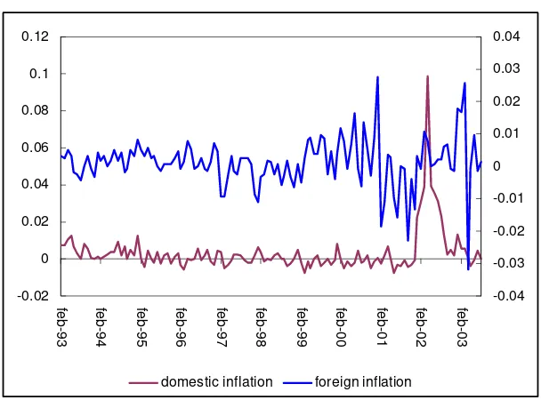
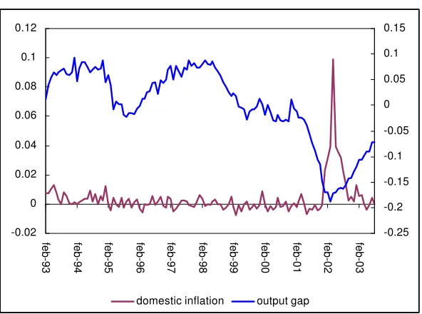
sample. Figures 1 to 3 illustrate the relationship between domestic inflation and its

main determinants over the period of analysis.

Figure 1: Domestic Inflation and nominal devaluation

-0.02 0 0.02 0.04 0.06 0.08 0.1 0.12

feb-93 feb-94 feb-95 feb-96 feb-97 feb-98 feb-99 feb-00 feb-01 feb-02 feb-03 -0.3

-0.2 -0.1 0 0.1 0.2 0.3 0.4 0.5 0.6 0.7

domestic inflation nominal devaluation

Figure 2: Domestic and Foreign Inflation

-0.02 0 0.02 0.04 0.06 0.08 0.1 0.12

feb-93 feb-94 feb-95 feb-96 feb-97 feb-98 feb-99 feb-00 feb-01 feb-02 feb-03 -0.04

-0.03 -0.02 -0.01 0 0.01 0.02 0.03 0.04

Figure 3: Domestic Inflation and the Output Gap

-0.02 0 0.02 0.04 0.06 0.08 0.1 0.12

feb-93 feb-94 feb-95 feb-96 feb-97 feb-98 feb-99 feb-00 feb-01 feb-02 feb-03 -0.25

-0.2 -0.15 -0.1 -0.05 0 0.05 0.1 0.15

domestic inflation output gap

Figure 1 shows the weak response of domestic inflation to the sharp nominal

devaluation and also how rapid it decelerated, following the stabilization of the nominal

exchange rate converging to its average during Convertibility. Figure 3 depicts the

relationship between the output gap and domestic inflation, showing the persistent

negative values of the output gap since April 1999, reaching a trough in February 2002,

after the devaluation in January of the same year. Inflation had a weak response to the

deep and lasting decay in economic activity and prices even showed a deflationary

tendency. Although there was a positive response to the nominal devaluation of

January 2002, as said before, inflation rapidly slowed down, probably due to the high

levels of unemployment and capacity utilization.

4.2. Estimation results

We estimate a reduced form of the “Hybrid New Keynesian Phillips Curve”, given by

equation (8), which provides interesting information about the dynamics of inflation. In particular the relevance of forwardness in price setting behavior by firms is an issue

that has not been investigated yet for Argentina. Rather than imposing the verticality of

the Phillips Curve in the long run, we test for it, specifying (8) as follows

) ' 8 ( x

e )

(

E * _{t t t}

t 1 t t 2 1 t 1

t φπ φ π γπ λ δ ε

We then estimate equation (8’) using GMM. Nine lags of all variables are used as instruments. To test for the robustness of our results, we conducted several

estimations of (8’) using the different specifications for matrix HAC ∧

Ω described in section 3. As can be seen from Table 1 the estimations are quite robust to changes in

the specification of HAC ∧

Ω . For this reason, our preferred form for HAC ∧

Ω is Variable Newey – West, which selects the band-with based on the autocorrelation in the data

and thus is the more flexible one. Tests for over-identifying restrictions, applied to each

of the estimations confirm that the instruments are valid in all cases.

Table 1. Estimation results

GMM estimates Newey-West (nw) Andrews (2.88) Variable

Fixed (4) Newey-West (9)

φ1 0.561700 0.560719 0.450607

Std. Error 0.0493 0.0654 0.0337

φ2 _{0.160795 0.135870 0.207878}

Std. Error 0.0358 0.0598 0.0252

δ ∗ 0.015912 0.017891 0.016610

Std. Error 0.0049 0.0058 0.0028

γ ∗ 0.38148 0.373438 0.325374

Std. Error 0.0930 0.1047 0.0546

λ ∗ 0.028426 0.033837 0.025128

Std. Error 0.0059 0.0075 0.0041

J-statistic 0.117078 0.140565 0.094189

* These coefficients correspond to the first lag of foreign inflation and nominal devaluation respectively.

As said before, we concentrate on the results of the model using the Variable

Newey-West specification, which is also the one that yields the better estimation in terms of the

individual significance of variables and the overidentifying restrictions test. A first

important finding is that there is a significant forward-looking component in price

formation. The backward looking component is also relevant, but the relative values of

φ1and φ2 indicate more weight of the backward looking component.

4

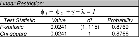
We checked for

the validity of imposing verticality in the long run, and we couldn’t reject the null (see

Table 2).

4 _{We tested for equal weights of the backward and forward looking components and the hypothesis was}

Table 2: Testing for linear restrictions

Linear Restriction:

Test Statistic Value df Probability F-statistic 0.0241 (1, 115) 0.8769

Chi-square 0.0241 1 0.8766

φ1+ φ2 +γ+λ= 1

Given that we are extending the model to the case of a small open economy it is

interesting to observe that changes in foreign inflation and nominal devaluation have a

significant effect on domestic inflation. Inflation responds to lagged values of both,

nominal devaluation and foreign inflation. While the response of domestic prices to

changes in foreign inflation is quite important, of around 0.33, its response to nominal

devaluation, although significant, is much weaker. These results have to be taken

cautiously, since most part of the sample we are considering here corresponds to the

“Convertibilidad” period over which the peso was fixed to the dollar. We also find a

weak response of domestic inflation to changes in the output gap. This is frequent

empirical finding in the literature on short-run inflation dynamics.

Summing up, our results suggest that a hybrid representation of the “New Keynesian

Phillips Curve” adequately describes inflation dynamics in Argentine over the period

1993-2003. The estimates indicate that both components, forward and

backward-looking appear to be significant in price formation decisions. Finally, we find strong

evidence of verticality in the long run.

5. Conclusions

Recent developments in the empirical modeling of short-run dynamics of inflation

assume inter-temporal optimizing behavior by non-competitive firms. The empirical

relevance of persistence in inflation dynamics has led to introduce backwardness in

these models by assuming that a portion of the firms could follow a backward-looking

rule. The resulting model is known as the “Hybrid New Keynesian Phillips Curve”.

Using GMM, we estimate a “Hybrid New Keynesian Phillips Curve” for Argentina over

the period 1993-2003. We extend the basic model to the case of a small open

economy, allowing nominal devaluation and foreign inflation to play a role in domestic

prices setting. We find that both components, forward and backward are relevant to

explain the dynamics of domestic prices, although the backward-looking component

inflation are also significant to explain domestic inflation behavior, being the response

of inflation to the second more intense. The output gap, although weak, has a

significant effect on inflation. We cannot reject verticality of the Phillips Curve in the

References

Andrews, D., 1991. “Heteroskedaticity and Autocorrelation Consistent Covariance

Econometrica, 59, 817-858.

Bakhshi. H. et.al. 2002. “Price-Setting Behavior and Inflation Dynamics”. Mimeo. Bank

of England.

Calvo, G. A., 1983. “Staggered prices in a utility maximizing framework”, Journal of Monetary Economics 12, 383-398.

Dotsey, M., 2002. “Pitfalls in Interpreting Tests of Backward looking pricing in New

Keynesian Models”, Economic Quarterly. Federal Reserve Bank of Richmond. Vol. 88/1. Winter 2002.

EViews, 2000. User’s Guide, Quantitative Micro Software, LLC.

Favero, C., 2001. Applied Macro-econometrics, Oxford University Press.

Fischer, S., 1997. “Long Term contracts, rational expectations, and the optimal money

Journal of Political Economy 85, 163-190.

Galí, J. and M. Gertler, 1999. “Inflation Dynamics: A structural econometric analysis”,

Journal of Monetary Economics 44, 195-222.

Guerrieri, L., 2002. “The inflation persistence of staggered contracts”, Board of Governors of the Federal Reserve System, International Finance Discussion Paper No 734.

Hamilton, J., 1994. Time Series Analysis, Princeton University Press.

Hansen, L.P., 1982. “Large Sample Properties of Generalized Method of Moments

Econometrica 50, 4, 1029-1054.

Lindé, J., 2002. “Estimating New-Keynesian Phillips Curves: A Full Information

Newey, W. and K. West, 1994. “Automatic Lag Selection in Covariance Matrix

Review of Economic Studies 61, 631-653.

Svensson, L.E.O., 1998. “Open-Economy Inflation Targeting”, NBER Working Paper

No. 6545, May.