The effects of individual characteristics on the distribution of college performance

THE EFFECTS OF INDIVIDUAL CHARACTERISTICS ON THE DISTRIBUTION OF COLLEGE PERFORMANCE

WALTER SOSA ESCUDERO, PAULA INES GIOVAGNOLI AND ALBERTO PORTO

RESUMEN

Las interacciones entre los determinantes observables e inobservables del éxito educativo implican que los primeros tienen un efecto heterogéneo en el rendimiento. Para cuantificar estas interacciones, se estima un modelo de regresion por cuantiles utilizando microdatos de universidades públicas argentinas. Los resultados muestran que los factores que contribuyen positivamente al rendimiento son mayores en las colas inferiores de la distribución. Políticas que mejoran el rendimiento de quienes se encuentran en la parte inferior de la distribución condicional tienen un efecto dual de incrementar los rendimientos absolutos y de reducir las disparidades debido a un mayor efecto en este grupo.

Clasificación JEL: I21

Palabras Clave: Argentina, rendimiento educativo, educación universitaria,

regresión por cuantiles.

ABSTRACT

Interactions between observed and unobserved determinants of educational success imply that the former have a heterogeneous effect on performance. To quantify these interactions, a quantile regression model is estimated using a database of students at public universities in Argentina. The empirical results show that all factors which contribute positively to performance are stronger in the lower end of the distribution. Hence, policies that enhance the possibilities of students in this part of the conditional distribution have the dual effect of increasing absolute performance and reducing disparities due to their stronger effect in this group of students.

JEL Classification: I21

Keywords: Argentina, educational performance, higher education, quantile

THE EFFECTS OF INDIVIDUAL CHARACTERISTICS ON THE DISTRIBUTION OF COLLEGE PERFORMANCE 1

WALTER SOSA ESCUDERO, PAULA INES GIOVAGNOLI AND ALBERTO PORTO 2

I. Introduction

Considerable space has been awarded in the social and human sciences to the question of how individual characteristics impact on educational performance. A quantification of how student-specific factors affect educational success is crucial to explain disparities in educational achievements, and to design and evaluate specific actions aimed at promoting upward social mobility. This requires accurate empirical models that link educational performance to its observable determinants.

As has been well documented, mostly due to the inherent complexity of the problem, available models are still far from this goal, which is usually reflected in their very poor goodness-of-fit performance. For example, Betts and Morell (1999) in a related study for the University of California at San

Diego, obtain R2 _{coefficients of around 0.15, using a rich dataset of 5,623}

students3_{. This means that even after conditioning on many observable aspects}

that determine success, individuals still differ substantially due to unobserved factors. Consequently, the correct way to assess the effect of an observable variable on performance is to think about how changes in this specific factor

affect the conditional distribution of performances.

1 _{We thank Luciano Di Gresia, Graciela Molino, Roger Koenker, Maria Victoria Fazio and two} anonymous referees for useful interactions and comments. This research project was part of the PICT 2002 program (02/11297) of Argentina’s Agencia Nacional de Promocion Cientifca y Tecnologica. All omissions and errors are our responsibility.

2 _{Walter Sosa Escudero: Universidad de San Andrés. Paula Inés Giovagnoli: London School of} Economics and Universidad Nacional de La Plata. Alberto Porto: Universidad Nacional de La Plata. Corresponding author: Paula Giovagnoli, London School of Economics and Political Science, Houghton Street, Tower Two Building, 5th Foor, Room V512. London WC2A 2AE, United Kingdom, e-mail: p.i.giovagnoli@lse.ac.uk.

As a simple example consider the effect of father’s education. The distribution of performances conditional on observed factors, including father’s education, still presents substantial variability due to the non-trivial role played by unobservables, hence, even within a group of individuals with the same observed characteristics, we will find students with bad, regular, or good educational performance. It is natural to expect that the whole conditional distribution of performances gets shifted to the right when, other things equal, we consider students with better educated fathers. In the extreme case where additional father’s education shifts the whole conditional distribution to the right without altering its shape, the effect of increasing

father’s education on the mean performance captures everything there is to

know. In such a context, and under some simplifying assumptions, a standard regression model gives the desired answer: the coefficient of fathers’s education in a linear regression captures the effect on expected performance and, under these circumstances, on performance in general. This situation naturally arises when father’s education is independent of non-observables in the determination of performances, hence, movements in father’s education imply pure location shifts of the conditional distribution of performances. But given the non-trivial role played by unobservables in these models, we cannot discard the possibility that movements in father’s education interact with factors not included in the model in a non-obvious way. It might be the case that father’s education play a more important role in children less inclined towards study, and a mild effect on those more motivated. In this case, the ‘mean effect’ of father’s education is positive but does not represent anybody in the population: it overestimates the effect on individuals with high propensity towards study, and underestimates the situation of the less motivated students.

lead careless observers to the wrong conclusion that age does not have any effect, ignoring its impact on the dispersion.

The main goal of this paper is to measure the effect of observable individual characteristics on the whole conditional distribution of

performances using recent quantile regression methods. We are not trying to

isolate the causal effects of the observable variables included in the model, but instead our focus is on the differences between the incremental effects of the variables at the different quantiles of the conditional performance distribution. There are three main reasons why the quantile regression approach is relevant. First, it complements standard ‘educational production function’ studies by exploring effects beyond those on the conditional mean. This is important since educational policies are usually expected to have an impact on those students who face relatively more difficulties, so extrapolating the effect of the average individual may induce considerable biases in the assessment of such policies.

Second, mean effects are seldom informative about the distributive impact

of policies. The presence of heterogeneous effects suggests that changes in specific characteristics may have the effect of improving everyone’s performance but also of altering the shape of the distribution of these performances. Quantile methods provide an informative picture of these distributive effects. This is a particularly relevant issue since education is

explicitly seen by many social actors as an active equalizing policy4_{. For}

example, and as a preview of some empirical results, having attended a private

secondary school (as opposed to public) has a positive effect on performance for individuals around the center of the distribution of their unobservable factors, and no effect for those extremely good or bad. Then, having attended a private secondary school makes the distribution of performances more

asymmetric, a subtle but relevant effect improperly summarized by the

‘average’ effect.

Third, distributive results become crucial when the screening perspective of

schooling is emphasized. In this context, what matters is the capacity of the educational system to provide information about the relative abilities of individuals, and hence, as stressed by Hanushek in his classic survey ‘...more attention should be directed towards the distribution of observed educational outcomes (instead of simply the means)...’ Hanushek (1986, pp. 1153).

The analysis of the relationship between educational outcomes and observed factors has been investigated more intensively at the elementary and secondary levels, leaving ample room for contributions aimed at the higher education level. The empirical application of our paper exploits a comprehensive census data set that covers all students attending public universities in Argentina in 1994. Public higher education in Argentina has been operated as a free and unrestricted access system -in general without entrance examinations- during most of the last twenty years, providing a rather unique source of sampling variability. Students entering university come from diverse socio-economic backgrounds. Additionally, in some popular degree programs like Accountancy or Law, university rules are very flexible and

leave the student s progress up to themselves. This results in very different

performances among students of the same cohort, adding greater value to our data set. To the best of our knowledge, this is the first paper that takes advantages of these particular features.

in light of these results, we emphasize the use of quantile methods to study

how individual characteristics impact on performance. As mentioned before,

the literature on higher education and performance is relatively scarce as compared to that related to elementary and secondary education; a representative study of this literature is Naylor and Smith (2004), who study the determinants of college performance for the United Kingdom and Di Gresia et. al. (2007), Porto (ed.) (2007) for the case of Argentina.

The rest of the paper is organized as follows. The next section discusses the econometric strategy used to recover the effects of observed variables on conditional distributions, while linking this study to previous literature on the subject. Section III presents the data set used in the empirical part and details the particular aspects of the Argentinean higher education system which are relevant for the purposes of this paper. Section IV presents the econometric results, and Section V concludes.

II. Exploring distributive effects through quantile regressions

As mentioned in the Introduction, non-trivial distributive effects of observed factors arise when they interact with non-observables. This section presents a simple structure for these interactions and proposes the use of quantile regressions to model them.

A. Interactions between observed and unobserved factors

The educational production function approach, originated in the famous ‘Coleman Report’ and reviewed extensively by Hanushek (1986), models educational performance as the outcome of transforming ‘inputs’ into

educational ‘outputs’ in a production function fashion5_{. A stringent empirical}

limitation of these models is that the vector of inputs includes a myriad of unobserved individual specific factors which may play a non-trivial role. To the point, in his landmark paper Hanushek (1979) states that ‘...the most consistent and obvious divergence of the empirical models from the conceptual models is the lack of measurements for innate abilities’. In educational production functions, these abilities play a role similar to that

played by ‘entrepreneurial factors’ in standard micro-theory production functions, in the sense that they represent unobserved factors that imply different profits for different firms (individuals, in the case of education) and that may alter the way observed factors affect production.

Consider a simple, individual specific, production function

y

i=gi(x) (1)

that represents the maximum educational outcome y that an individual i may

produce with inputs x. In general this function is not homogeneous of degree

one since each person has its own set of fixed ‘innate abilities’. As clearly stressed in the standard microeconomic theory (i.e., Mas Collel, et al., 1995, pp. 134-35), production functions reflect technologies, not limits on resources, hence the individual specific production function is better represented by

y

i=g(x,ui) (2)

where u represents unobserved factors that once fixed at a particular level

describe how x is transformed into y for a particular person.

As it is well known in the literature, u is far from playing a minor role in

explaining educational disparities. Even when the dimension of x is large so as

to include a multitude of individual and institution specific factors, u still

contains abundant unobserved information about the psychological and

motivational characteristics that make individuals differ in their performance6_.

Hence it is risky to proceed by making strong assumptions about the role

played by u in the production process.

In particular, we are concerned with the possible interactions between unobserved and observed factors. This is a question related to the specific form

of g(x,u). Using a translog specification, Figlio (1999) explores interactions

among observed factors by testing the statistical significance of interactive

terms. But if interest lies in exploring interactions between observed and

unobserved factors we cannot rely on such a strategy.

B. The quantile regression approach

Consider the following general, possibly non-separable, production function:

y = g(x,u) (3)

and, to simplify notation, consider the case where x is a single observed

explanatory factor. Our interest is in exploring whether y/x varies with

different levels of u, and ‘separability’ or ‘no-interaction’ means that this

derivative is constant across the different levels of u. Since u is not observed

by the analyst it is awkward to speak about its absolute levels. Instead, it seems more convenient to consider a standardized relative notion, like its

quantiles, that is, levels of u that are deemed as ‘high’ based on the (relative)

notion that a large proportion of its possible values lie below them7_.

In this context the starting point is how much of y can be produced when u

is set at its -th conditional quantile given x, that is,

g(x,Q_u|x()) (4)

where the notation stands for the -th quantile of the distribution of a

random variable z conditional on x8. If, as is standard for any production

function, we assume that g(x,u) is monotonic in u when x is fixed, and since

quantiles are equivariant under monotonic transformations (i.e.,

Q_h(z)()=h(Q_z()) for any monotone function h(.)), then

g(x,Q_u|x()) = Q_g|x(g(x,u))() = Q_y|x() (5)

Hence how much can be produced when u is set at any relative level

measured by its conditional quantiles coincides with the -th conditional

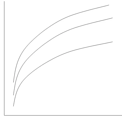
quantile of performances. In the simple case where x is a single production

factor, in the space (y,x) this corresponds to a family of production functions

indexed by the conditional quantiles of u. Figure 1 illustrates this point where

each curve corresponds to for increasing levels of .

Consequently, our measures of interest are the partial derivatives of these

production functions for different relative levels of u, . Quantile

regression models are specifically designed to estimate these derivatives. Using the chain rule in (5)

7 _{Roemer (1998, pp.10) adopts a similar relative characterization when he uses centiles to} measure effort.

8 _{This argument follows Chesher (2003) who studies the identification of general non-separable} functions.

g(x,Q_u|x())

Q_z|x()

Q

Q_y|x()

x =

g(x,u)

x +

g(x,u)

u

Q_u|x

x (6)

In this context ‘separability’ means that g(x,u)/x does not depend on the

levels of u and that Q_u|x/x is zero, that is, u is independent of x.

As an illustration consider the linear case

y = ₀+ ₁x + u, (7)

so

Q_y|x() = ₀ + ₁x + Q_u|x() (8)

If u is independent of x

Q_y|x()

x =

y

x = 1, (9)

a constant, since there is no explicit interaction between x and u and since u

and x are independent.

The simplest specification that allows for these type of interactive effects is provided by the standard linear quantile regression model

g(x,Q_u|x()) = Q_y|x() = () + () x (10)

where () is any function. This implies that for any fixed , is a

linear function with slope (). Interactions arise due to the fact that for any

given x the slope of these lines is allowed to vary across the conditional

quantiles of u. The null hypothesis of ‘no-interaction’ corresponds to the case

where all slopes are equal, H₀:() = ₀.

Based on a sample of independent, though not necessarily identically distributed observations, coefficients of this model are estimated for several quantiles using the standard Koenker and Bassett (1978) estimator that solves:

_{() = argmin}

_

i=1

n

_(y_ix_i' b()), (11)

. Basic inference, like individual significance tests and confidence intervals, is handled as follows. We estimate the vector of

unknown coefficients for a grid of M equally spaced quantiles .

g(x,Q_u|x())

_(z) z(I (z<0)), (0,1)

(x_i,y_i), i=1,,n



Let be each of these vectors of coefficients, and let be their population counterparts. Collect all coefficients for all chosen quantiles as and . Under the assumption of a random and independent sample (not necessarily identically distributed) and under standard regularity conditions,

n(_n₀) d

N(0,V_n) (12)

where V_n is an MKMK block diagonal matrix with blocks:

V

n(m ,j) = [mjmj ]Hn(m) 1

J

nHn(j)

1 ₍₁₃₎

with

J_n=(1/n)



i=1

n

x_ix_i' (14)

H_n() = _nlim_ 

i=1 n

x_ix_i'f_i(F_i1()) (15)

and stands for the conditional density of . is estimated using the Koenker-Hendricks procedure. We refer to Koenker (2005) for further details.

Linear hypothesis of the type , where R is a qMK matrix

and r a q vector, can be evaluated through the statistic:

T_n=n(Rr)'[RV_n1R']1(Rr) (16)

which is distributed as 2₍

q) asymptotically under H0 , where q is the rank of R. This allows several configurations like individual or joint significance of variables, or the ‘homogeneity’ assumption that coefficients are equal across quantiles.

Consider the homogeneity assumption where all

slopes are equal across all quantiles. The previous approach handles this

hypothesis through evaluating it at a discrete grid of selected quantiles. Koenker and Xiao (2002) propose appropriate tests for this hypothesis along a

continuous range for . The homogeneity null is usually referred to as the

‘pure location shift’ hypothesis, since under it variables have the effect of shifting the whole conditional distribution without altering its shape. A less drastic hypothesis is the pure ‘location-scale’ hypothesis which implies a particular form of heterogeneity where variables shift the conditional

H_n()

H₀ : R₀r = 0

H₀ : () = ₀ ,(0,1)

(

m)

_(

m)

_(_(

1)'(M)')' ((1)'(M)')'

distribution while altering its scale in a simple ‘heteroscedastic’ fashion. We implement both tests, and refer to Koenker and Xiao (2002) for technical details.

III. Data and main features of the higher education system in Argentina

We base our study on the CEUN (Censo de Estudiantes de Universidades Nacionales), a national census data set that covers all college students enrolled at the 31 national universities in Argentina in October 1994, amounting to approximately 615,000 students. This database includes detailed information on several personal and household socio-economic characteristics, as well as college performance for each student in the sample.

Because of its distinguishable institutional features, the sampling variation in our data is ample, offering a rather unique empirical opportunity to study the determinants of college success. Specifically, the system of public universities in Argentina has a long tradition of promoting equality of opportunities by providing free and unrestricted access to higher education. Free-tuition remained even after the Higher Education Law was passed in 1995, which provides universities with full autonomy over their administration, internal resource allocation, staff management, and student access. According to this Law, it is up to the universities to decide whether or

not they want to charge fees9_{. Nevertheless, the great majority of universities}

do not charge tuition and, in general, there are no limiting entrance examinations.

Our data is also less vulnerable to the negative effects of the selection mechanisms present in most universities, specially those in the American or British systems where strong competitive schemes determine access. For instance, in the US or the UK, students must achieve a minimum score at secondary education level in order to apply to a specific university. This restriction influences the allocation of students to particular universities, biasing correlations between educational performance and students in such samples.

Other countries in Latin America or Europe (for example, Germany) also promote free access by keeping tuition levels at relatively low or zero cost, but the case of Argentina is important since tuition-free is, in general,

simultaneously combined with free entrance, independent of previous student performance in secondary school or pre-examinations.

Compared to other countries, higher education coverage in Argentina ranks among the highest. According to the official Permanent Household Survey from May 2003, 65% of young people aged 18-29 years old who completed secondary school started university, and 20% of them are in the lowest quintile

of the equivalized household income distribution10 _{compared with 32% in the}

highest quintile, showing that beneficiaries of public university education

come from families located in different parts of the income distribution.11

Our dataset provides evidence that students attending higher education come from a diverse socio-economic background and constitute a heterogeneous group. Moreover, additional statistics for a subgroup of our data show that poor people do not only start university but they also obtain a degree- albeit with lower chances than those who come from the richer families. For instance, following a cohort of Accountancy students at National University of Rosario since 1991 up to 2001, Giovagnoli (2005) noticed that 20.4% of those who graduated had fathers with primary education or less.

An additional characteristic that makes Argentina’s public higher education system an attractive case is that students in most programs face highly flexible schedules and mild requisites that allow them to proceed at their own pace. Hence a cohort of students could advance very dissimilarly along its academic path without being penalized, leaving ample room for individual characteristics to play a role as determinants of performance. As we will show later, data confirms this pattern. Specifically, for reasons explained below, focusing on a cohort of students who started university in 1991 and measuring their performance by 1994, we observe high variation.

The choice of a particular measure of performance is a delicate issue subject to much debate. Some authors draw on measures such as GPA’s (Betts and Morrell, 1999), the Graduate Record Examination (GRE) (McGuckin and

10 _{Equivalized income takes into account the fact that food needs are different across age groups} - leading to adjustments for adult equivalent scales - and that there are household economies of scale.

Winkler (1979)) or the estimation of potential incomes (Card and Krueger (1996)), to give a few examples. These measures are unavailable in the CEUN data set. Nevertheless, there are no theoretical or empirical reasons to consider that one indicator dominates the others, in fact, there is a vast literature revising the weaknesses and the strengths, supporting the use of different measures - for a rich and extensive discussion on the issue see Hanushek (1979, 1986). In this paper we measure performance as the number of courses passed from the beginning of the program (as we will be working with the cohort of students enrolled in 1991 observed in 1994, we will measure number of courses passed after 4 years of study). In the context of understanding education as a production process already discussed in Section II this is a measure of average productivity. Thus, a student who passes more courses per year demonstrates greater productivity - i.e. has a better performance - than another one who contemporaneously started university and passed less courses. The former student will be able to incorporate human capital in a shorter period of time leading to earning incomes at an earlier point in the life-cycle.

With respect to the choice of explanatory variables, the underlying theory is not explicit about any particular choice, hence data availability has played an important role in this decision. Following previous research (Hanushek (1979, 1986), Naylor and Smith (2004) and Betts and Morell (1999)), we will consider the inclusion of particular variables which can be grouped into four main types: (i) the student’s demographic variables (gender, age); (ii) the student’s family background (parent’s education); (iii) the student’s chosen factors such as the decision to work or not, city of residence/or commuting and marital status and (iv) type of school that the student attended prior to enrolling in university (public or private secondary school, type of orientation

- commercial or others12).

Our empirical analysis is focused on the two most popular programs, Law and Accountancy, at the four largest universities: University of Buenos Aires (UBA), National University of Cordoba (UNC), National University of Rosario (UNR) and National University of La Plata (UNLP). The choice of

this particular sub-sample is based on the usual trade-off between increased information and heterogeneity: more programs and universities provide more sample points at the potential cost of introducing heterogeneities between schools and programs that may obscure the goals of our analysis. Students at these four universities concentrate more than 50% of total enrollment at national universities in the country and, out of these, approximately 30% study Accountancy or Law (among 900 other career options).

Interestingly, these programs are quite homogeneous among national universities of the country because an important part of their syllabi is related to national laws and codes, and their professional practice is subject to strict

regulations13_{. This allows us to pool observations from different universities}

and increase precision without introducing heterogeneities at university level14_.

From the total number of individuals studying Accountancy and Law in the 1994 Census, we focused on students who enrolled during 1991, who are approximately 8.000. As these programs have a nominal length of at least five or six years, the very good students of this cohort were in their fourth year at the time of the census. More recent cohorts (those who entered after 1991) passed less courses at the time of the census, hence their measure of performance is a less precise indicator. In the extreme case, the 1994 cohort has only passed a few number of courses, thus the average number of courses passed may be a very poor predictor of overall performance. On the other hand, older cohorts are not correctly represented since their best students may have finished college in the expected five years of study and are naturally not present at the moment the census was conducted.

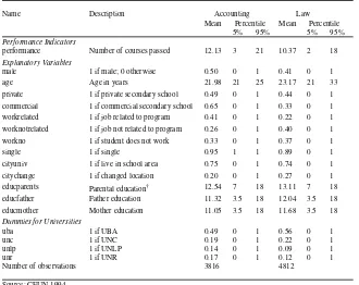
Table 1 shows descriptions and summary statistics for the variables included in our dataset. The performance indicator reveals that after four years students in Accountancy programs passed, on average, 12.13 courses, hence

13_{Unlike the US system, the professional practice of lawyers and accountants in Argentina} requires an undergraduate degree in Law or Accountancy, respectively. For example, to become a professional accountant a student must obtain an undergraduate degree in Accountancy and then obtain a professional license in the province where she/he is interested to practice her/his profession. The license is awarded automatically to every graduate, without exams, since it is understood that the professional evaluation has already taken place at the University. Accountancy norms are quite homogeneous across different provinces. The case of lawyers is similar.

the average productivity is around three courses passed per year. Note that in the case of Law, the nominal duration of the program is one year more than Accountancy, while the number of courses is similar. Then, by 1994 Law students should have passed fewer exams than those in Accountancy.

While the same proportion of males and females attend Accountancy, females are relatively overrepresented in the Law program (59%). The latter sample has slightly older and non-single students, and 56% of the students come from a public secondary school. In Law there is a significant smaller proportion of students than in Accountancy who previously attended a secondary school with commercial orientation compared with those who attended a different secondary school orientation (33% versus 65%).

Labor market variables suggest a very dissimilar composition in each program related to the kind of job students have. Although around 35% of both accounting and law students said they did not have a job by 1994, working groups are different between the programs. While 41% of accounting students have a job related to their careers, only 22% of Law students have a job linked to their profession.

Regarding the characteristics of student’s fathers, in Accountancy, they have, on average, 11 years of formal education, which corresponds to incomplete secondary school. Fathers of students in Law are slightly more educated. Finally, the proportion of students in each university highlights the relevance of UBA in the total sample - 56% (49%) of Law (Accountancy) students are from UBA, with UNC being the second largest in terms of the students in the sample.

IV. Estimation results

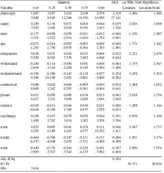
We have estimated a basic linear quantile regression specification using the log of performances as the dependent variable, for Accountancy and Law students respectively, pooling the information from the four universities considered, and including dummy variables by universities.

is a location shift and a location-scale shift, respectively. In the bottom of these two columns we present the test statistics of the global hypothesis of location shift and location-scale shift. These tests strongly reject the null of homogeneity or pure location effects, stressing our initial point that the effect of observed factors is heterogeneous across the quantiles of unobserved factors, suggesting the presence of non-trivial interactions, in the sense discussed in section II.

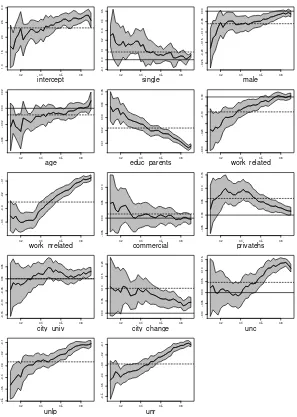
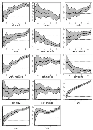
Figures 2a) and 2b) present these results graphically, for Accountancy and Law, respectively. Each small picture presents the effect of each explanatory

variable on the -th quantile of the conditional distribution for a finer grid of

quantiles (=0.1,0.11,…,0.89,0.9). The solid line shows the effect at each

quantile and the shaded area represents a 90% confidence interval. The dotted horizontal line represents the OLS estimation. When relevant, the solid horizontal line simply indicates zero.

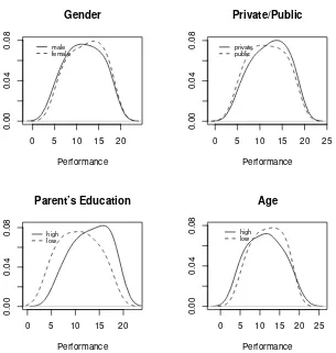
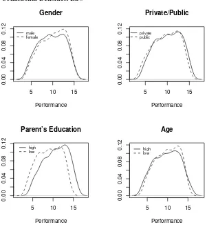
Now we turn to the analysis of the effect of individual factors. We will start by commenting results for Accountancy and then highlight differences and similarities with respect to Law. The gender dummy has a negative and significant effect in the mean OLS based model for Accountancy, suggesting that the expected performance of males is around 6% lower than that of females. Nevertheless, quantile regression results reveal that the effect is stronger in the lower levels of the conditional distributions, decreasing in absolute values and becoming statistically insignificant at the upper level. Figure 3 illustrates this point by showing the conditional densities of performances of Accountancy students, for males and females, with all the

remaining covariates set at their mean levels.15 _{Even though the effect is in}

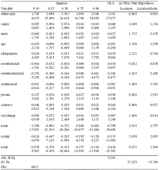
general mild, the estimated densities show that the conditional distribution of males’ performances have a larger left tail, so gender differences appear mostly in this range and not among those with higher performance. The case of Law students, illustrated graphically in Figure 4, is slightly different, since the gender dummy is significant only in the middle part of the conditional distribution and insignificant in the extremes, consequently, the conditional distribution of performance for females is skewed to the right as compared to that of males. Though the effect is mild, it appears clearly in Figure 4.

An important issue is the effect of having private versus public secondary education. The positive OLS based effect is actually a consequence of a

positive and significant effect in the center of the conditional distribution of performances, in spite of being insignificant in the extremes. There are several intuitions behind this result. Public secondary schools in Argentina are, overall, perceived to be of lower quality than private ones since they usually receive students with less favorable socioeconomic backgrounds, except for a few which are very traditional and manage to attract the very best students. Consequently, the fact that effects are nil in the extremes and positive in the center is compatible with the idea that once in college students from public secondary schools have a markedly negative asymmetric distribution of performances, most of them in the lowest tail of the distribution and relatively few at the top. The opposite results appear in the case of those with private education: most students have a good performance and relatively few of them have extremely bad performances. In either case the very good students, in terms of their performances, do not seem to have benefitted from having attended one type of school or the other, and the same happens in the other extreme. This result is illustrated graphically in Figure 3, where the conditional densities of performances are plotted for students with private and public secondary education. The central part of the conditional distribution for those with private secondary school education appears shifted to the right, with the extremes unaltered, compared with those students with public secondary school background, compatible with positive effects in the middle and nil effects in the extreme. The case of Law students is different since private education has a strong effect in the bottom of the conditional distribution, decreasing monotonically and having a rather constant effect beyond the quantile 0.4.

students with more educated parents is shifted to the right and more skewed to the left, consistent with the effect of parental education being positive but decreasing across the quantiles.

Age effects are interesting. OLS estimations are insignificant for both accountants and lawyers, suggesting that age has no effect on the conditional mean of performances. Nevertheless, the age effect by quantiles ranges monotonically from being significantly negative in the lower levels to slightly

significant and positive in the upper quantiles; a very similar and stronger

effect is found for the case of lawyers. This seems to be indicative of a pure

scale effect where, other things equal, classes with older students are more

disperse in the sense that age plays a positive role for those in the upper tail of the distribution of non-observables and a negative one for those conditionally in the bottom. This is consistent with the intuition that good but otherwise older students may be more focused and mature about what they expect from their education (the positive effect of age) and hence perform better than those in the bottom (badly motivated or low skilled) for whom age plays a negative role in their performance. This result can be seen in Figures 3 and 4, where we plotted the conditional distribution of performances for individuals who, at the moment of the census were 21 and 30 years old. Consequently, in spite of having similar locations, the conditional distribution of performances of older students is more disperse than that of younger ones. As mentioned in the Introduction, the insignificance of the age variable in the OLS mean model might lead careless observers to the wrong conclusion that age has no effect in performance, ignoring that it has a non-trivial effect on the dispersion, a fact that has important consequences since more heterogeneous groups may require a different pedagogical treatment than younger and more homogeneous ones.

Next we explore the effect of working while studying. Variables

work-related and work-not-related are dummy variables indicating with one,

working in related jobs does not have a significant effect above the median. These are very relevant results since they imply that career specific jobs do not compromise performance for Accountancy students with relatively good

performance16_{. The case of Law students is different. The dummy variable}

denoting jobs related to the career is never significant at all quantiles and in the OLS model. The effect of working in non-related jobs is similar to the one for accountants. This is a relevant result since it reveals that the dynamics of a career in Law is compatible with a job related to the practice of the Law without affecting performance, but also with the fact that students who do not work do not have a better performance than those who have jobs related to the career. The detrimental effect appears only in the case of those working in jobs not related to the career.

A much debated topic in the local literature is the relevance of the type of secondary education, where students who have the ‘commercial’ orientation are expected to have a relative advantage in Accountancy. Surprisingly the type of secondary school orientation has a homogeneous not significant effect on performances in both Accountancy and Law.

Marital status is homogeneously non-significant across most quantiles, and a similar result holds for Law students. Location variables have rather homogeneous effects, so quantile regression results do not add much to those revealed by OLS. Having to commute to attend college is not a relevant factor across all quantiles of the conditional distribution of performances. The fact that students reallocate to attend college has a homogeneously relevant and positive effect in performances, much in accordance with the idea that those willing to pay the fixed costs of reallocation are the relatively good students.

V. Conclusions

The main goal of this paper is to measure the effect of observable individual characteristics on the whole conditional distribution of performances. One of the main reasons for choosing this strategy is that in the case of educational policies it is necessary to complement the standard educational production function approach, by studying not only the mean

effects of observable variables but also their impact on the shape of the distribution of performances. This is relevant since educational policies are often expected to promote equality of opportunities and possibilities, and hence distributive outcomes matter. Also, if policy actions are oriented towards the less advantaged, or any other specific group, it is important to assess whether the impact of a policy measure is homogeneous for all students, or whether average effects are actually an imprecise summary of a more complex reality that may benefit certain individuals systematically more than others.

Heterogeneities arise from interactions between unobserved and observed factors in the production of educational outcomes. Quantile regression methods are shown to provide a flexible framework to model these interactions between observed and unobserved factors, which are the source of non homogeneous effects on performance that alter its conditional distribution in subtle ways improperly summarized by mean OLS based methods.

This methodological framework is adopted and applied to the case of college students in Argentina, whose social and institutional characteristics, that combine free access, a flexible schedule and a diverse socio-economic composition of its students, provide ample sampling variability making it a relevant case study.

References

Aráoz, A. (1968). “Comentarios sobre el trabajo del Dr. Julio H.G. Olivera

“La Universidad como Unidad de producción.””Económica, Vol. XIV (1-2):

111-114.

Betts, J. R. and D. Morell (1999). “The determinants of undergraduate grade point average: the relative importance of family background, high school

resources, and peer group effects.” Journal of Human Resources, Vol. 34(2):

268-293.

Card, D. and A. B. Krueger (1996). “The economic return to school quality.”

In Assessing Educational Practices: The contribution of Economics, eds.

W.E.Becker and W.J. Baumol. Cambridge, MA: The MIT Press.

Chesher, A. (2003). “Identification in nonseparable models.” Econometrica,

Vol. 71(5): 1405 - 1441.

Coleman, J.S., E. Campbell, C. Hobson, J. McPartland, A. Mood, F. Weinfeld

and R. York (1966). Equality of Educational Opportunity. Washignton DC:

US Government printing office.

Di Gresia, L., M.V.Fazio, A. Porto, L. Ripani and W. Sosa Escudero (2007).

“Academic Performance of Public University Students in Argentina.”

Well-being and Social Policy, Vol 3. (2): 67-100.

Ehrenberg, R. G. (2004). “Econometric studies of higher education.” Journal

of Econometrics, Vol. 121 (1-2): 19-37.

Eide, E. and M. Showalter (1998). “The effect of school quality on student

performance: a quantile regression approach.” Economics Letters, Vol. 58(3):

345-350.

Figlio, D. (1999). “Functional form and the estimated effects of school

resources.” Economics of Education Review, Vol. 18 (2): 241-252.

Giovagnoli, P. (2005). “Determinants in university desertion and graduation:

Gonzalez Rozada, M. and A. Menendez (2002). “Public university in

Argentina: subsidizing the rich?” Economics of Education Review, Vol. 21(4):

341-351.

Hanushek, E. (1979). “Conceptual and empirical issues in the estimation of

educational production functions.” Journal of Human Resources, Vol. 14(3):

351-388.

Hanushek, E. (1986). “The economics of schooling: production and efficiency

in public schools.” Journal of Economic Literature, Vol. 24(3): 1141-1177.

Koenker, R. and G. Bassett (1978). “Regression quantiles.” Econometrica,

Vol. 46(1): 33-50.

Koenker, R. (2005). Quantile Regression. Cambridge: Cambridge University

Press.

Koenker, R. and Z. Xiao (2002). “Inference on the quantile regression

process.” Econometrica, Vol. 70(4): 1583-1612.

Levin, J. (2001). “For whom the reductions count: A quantile regression

analysis of class size and peer effect on scholastic achievement.” Empirical

Economics, Vol. 26(1): 221-246.

Machado, J. and J. Mata (2005). “Counterfactual decomposition of changes in

wage distributions using quantile regression.” Journal of Applied

Econometrics, Vol. 20(4): 445-465.

Mas-Colell, A., M.D. Whinston and J.R.Green (1995). Microeconomic Theory.

Oxford University Press.

McGuckin, R. and D. Winkler (1979). “University resources in the production

of education.” The Review of Economics and Statistics, Vol. 61 (2): 242-248.

Naylor, R. and J. Smith (2004). “Determinants of educational success in higher

education”. In International Handbook of the Economics of Education, eds.

Geraint Johnes and Jill Johnes. Northhampton, MA: Edward Elgar.

Olivera, J.H.G. (1964). “Aspectos económicos de la educación.” Reprinted in

Olivera, J.H.G., (1967). “Die Universitat als Produktionseinheit.” Weltwirtschaftliches, Band 98, Heft 1.

Porto, A. (ed.) (2007). Mecanismos de admisión y rendimiento académico de

los estudiantes universitarios. Estudio comparativo para estudiantes de

Ciencias Económicas. La Plata, Argentina: Edulp.

Roemer, J. E. (1998). Equality of Opportunity. Cambridge: Harvard University

Appendix: Estimating Conditional Densities

In order to estimate the density of performances (y) conditional on a vector

x of explanatory variables, we first obtain a random sample from the

conditional distribution y|x. Machado and Mata (2005) suggest the following

procedure to obtain random numbers based on an estimated model for the

conditional quantiles. Assume that  is a random variable uniformly distributed

in (0,1). By the probability integral transformation theorem, if y|xF(Y|x)

Q_(y|x) = F_y1_|x() = x'()F_y|x.

Then, we can obtain a random sample of size J of y|x by first generating

uniformly distributed random numbers j , j=1,…, J , and then computing

, where are the estimates of the coefficients of the linear quantile regression for quantiles j , j=1,…, J. In our case, the vector x is set at convenient values. For example, in the comparison between students with

public vs. private secondary education, two samples were obtained by setting x

at their sample averages, and then switching the dummy variable for secondary school background from zero to one.

Once there is available a random sample of y|x, an estimate of the

conditional density is obtained by applying standard kernel methods on this random sample. The equivariance property of quantiles makes it straightforward to extend this mechanism to obtain random samples of any

monotone transformation of y. In our case, since the model is estimated for the

logs of performance, it is easy to see that is a random sample of the original variable in levels, when the model is estimated in natural logarithms.

exp(x'(_j)), j = 1,,J

_(

j)

x'(

Figure 1

Production Functions for Different Conditional Quantiles

0.2 0.4 0.6 0.8 1.0 1.5 2.0 2.5 3.0 intercept

0.2 0.4 0.6 0.8

−0.1 0.0 0.1 0.2 0.3 0.4 0.5 single

0.2 0.4 0.6 0.8

−0.25 −0.20 −0.15 −0.10 −0.05 0.00 male

0.2 0.4 0.6 0.8

−0.04

−0.02

0.00

0.02

age

0.2 0.4 0.6 0.8

0.01 0.02 0.03 0.04 0.05 educ_parents

0.2 0.4 0.6 0.8

−0.30

−0.20

−0.10

0.00

work_related

0.2 0.4 0.6 0.8

−0.4

−0.3

−0.2

−0.1

work_nrelated

0.2 0.4 0.6 0.8

−0.05

0.00

0.05

0.10

commercial

0.2 0.4 0.6 0.8

−0.05 0.00 0.05 0.10 0.15 privatehs

0.2 0.4 0.6 0.8

−0.15 −0.10 −0.05 0.00 0.05 city_univ

0.2 0.4 0.6 0.8

0.00 0.05 0.10 0.15 0.20 city_change

0.2 0.4 0.6 0.8

−0.10 −0.05 0.00 0.05 0.10 0.15 unc

0.2 0.4 0.6 0.8

−0.6 −0.5 −0.4 −0.3 −0.2 −0.1 unlp

0.2 0.4 0.6 0.8

−0.6 −0.5 −0.4 −0.3 −0.2 −0.1 unr Figure 2a)

0.2 0.4 0.6 0.8 1.4 1.6 1.8 2.0 2.2 2.4 2.6 intercept

0.2 0.4 0.6 0.8

−0.05 0.00 0.05 0.10 0.15 0.20 0.25 single

0.2 0.4 0.6 0.8

−0.10

−0.05

0.00

male

0.2 0.4 0.6 0.8

−0.020 −0.010 0.000 0.005 0.010 age

0.2 0.4 0.6 0.8

0.010 0.015 0.020 0.025 0.030 educ_parents

0.2 0.4 0.6 0.8

−0.15 −0.10 −0.05 0.00 0.05 work_related

0.2 0.4 0.6 0.8

−0.35

−0.25

−0.15

−0.05

work_nrelated

0.2 0.4 0.6 0.8

−0.10

−0.05

0.00

0.05

commercial

0.2 0.4 0.6 0.8

0.00 0.05 0.10 0.15 0.20 privatehs

0.2 0.4 0.6 0.8

−0.05

0.00

0.05

0.10

city_univ

0.2 0.4 0.6 0.8

−0.05 0.00 0.05 0.10 0.15 city_change

0.2 0.4 0.6 0.8

−1.4 −1.2 −1.0 −0.8 −0.6 unc

0.2 0.4 0.6 0.8

−0.8 −0.7 −0.6 −0.5 −0.4 −0.3 −0.2 −0.1 unlp

0.2 0.4 0.6 0.8

−0.7 −0.6 −0.5 −0.4 −0.3 unr Figure 2b)

Figure 3

Conditional Densities. Accountancy

0 5 10 15 20

0.00

0.04

0.08

Gender

Performance

male female

0 5 10 15 20 25

0.00

0.04

0.08

Private/Public

Performance

private public

0 5 10 15 20

0.00

0.04

0.08

Parent’s Education

Performance

high low

0 5 10 15 20 25

0.00

0.04

0.08

Age

Performance

high low

Figure 4

Conditional Densities. Law

5 10 15

0.00

0.04

0.08

0.12

Gender

Performance

male female

5 10 15

0.00

0.04

0.08

0.12

Private/Public

Performance

private public

5 10 15

0.00

0.04

0.08

0.12

Parent’s Education

Performance

high low

5 10 15

0.00

0.04

0.08

0.12

Age

Performance

Table 1

Variable Description and Summary Statistics. Accountancy and Law sample - Cohort 1991

Name Description Accounting Law

Mean Percentile Mean Percentile

5% 95% 5% 95%

Performance Indicators

performance Number of courses passed 12.13 3 21 10.37 2 18 Explanatory Variables

male 1 if male; 0 otherwise 0.50 0 1 0.41 0 1

age Age in years 21.98 21 25 23.17 21 33

private 1 if private secondary school 0.49 0 1 0.44 0 1 commercial 1 if commercial secondary school 0.65 0 1 0.33 0 1 workrelated 1 if job related to program 0.41 0 1 0.22 0 1 worknotrelated 1 if job not related to program 0.26 0 1 0.40 0 1 workno 1 if student does not work 0.33 0 1 0.37 0 1

single 1 if single 0.95 1 1 0.89 0 1

cityuniv 1 if live in school area 0.75 0 1 0.74 0 1 citychange 1 if changed location 0.20 0 1 0.27 0 1

educparents Parental education† _{12.54 7 18 13.11 7 18}

educfather Father education 11.32 3.5 18 12.04 3.5 18

educmother Mother education 11.05 3.5 18 11.68 3.5 18

Dummies for Universities

uba 1 if UBA 0.49 0 1 0.56 0 1

unc 1 if UNC 0.19 0 1 0.22 0 1

unlp 1 if UNLP 0.14 0 1 0.09 0 1

unr 1 if UNR 0.17 0 1 0.12 0 1

Number of observations 3816 4812

Source: CEUN 1994

Table 2a)

Quantile Regression Results. Accountancy

Quantile OLS (a) THn. Null Hypothesis :

Variable 0,10 0,25 0,50 0,75 0,90 Location Location/Scale

(Intercept) 1,687 2,057 2,418 2,649 2,578 2,318 1,406 1,546

3,888 8,945 12,288 18,330 16,995 17,141

single 0,250 0,136 0,071 0,018 0,044 0,079 2,026 1,008

3,552 1,609 0,910 0,336 3,433 1,526

male -0,177 -0,058 -0,059 -0,021 -0,012 -0,060 1,150 1,887

-3,101 -1,922 -2,916 -1,610 -1,354 -3,001

age -0,023 -0,014 -0,007 -0,002 0,009 -0,008 1,776 2,442

-1,293 -1,750 -0,978 -0,306 1,393 -1,891

educparents 0,038 0,031 0,020 0,013 0,008 0,022 2,321 2,670

5,559 8,092 7,579 7,885 6,948 8,824

workrelated -0,184 -0,114 -0,050 0,001 0,006 -0,084 1,335 2,943

-2,608 -3,144 -2,294 0,105 0,584 -3,488

worknotrelated -0,356 -0,390 -0,243 -0,115 -0,077 -0,254 3,439 3,518

-5,298 -10,108 -7,652 -5,801 -5,806 -9,562

commercial 0,048 0,042 0,006 -0,005 -0,004 0,014 1,488 1,022

0,860 1,262 0,293 -0,361 -0,404 0,641

private 0,023 0,099 0,080 0,034 0,015 0,062 2,028 1,750

0,417 3,231 3,850 2,629 1,656 3,065

cityuniv -0,045 -0,013 0,044 0,010 0,031 0,000 1,289 1,346

-0,664 -0,349 1,769 0,637 2,979 0,015

citychange 0,108 0,107 0,079 0,052 0,044 0,101 0,939 1,109

1,499 2,702 3,014 3,202 3,538 3,766

n.unc 0,023 0,007 0,041 0,119 0,111 0,046 2,047 1,733

0,292 0,188 1,423 6,577 10,352 1,611

n.unlp -0,464 -0,308 -0,247 -0,131 -0,111 -0,266 1,821 3,174

-6,357 -4,949 -7,619 -5,371 -6,509 -8,499

n.unr -0,440 -0,378 -0,264 -0,128 -0,101 -0,287 2,890 3,076

-3,983 -7,527 -7,543 -6,175 -7,982 -9,809

Adj -R Sq 0,102

(b) Tn 39,331 20,920

Obs 3.816

Note: t-values are given in the second line below each parameter estimate.

Table 2b)

Quantile Regression Results. Law

Quantile OLS (a) THn. Null Hypothesis : Variable 0,10 0,25 0,50 0,75 0,90 Location Location/Scale

(Intercept) 1,726 2,098 2,363 2,603 2,546 2,181 0,865 0,962

8,675 15,000 24,638 36,780 38,895 27,077

single 0,085 0,094 0,074 0,016 0,010 0,068 2,069 1,136

0,887 1,605 2,090 0,589 0,408 2,107

male -0,060 -0,063 -0,052 -0,021 0,018 -0,027 1,732 2,479

-1,353 -2,198 -2,982 -1,607 1,421 -1,605

age -0,010 -0,006 -0,002 0,000 0,006 -0,001 2,328 3,259

-2,324 -1,753 -0,698 0,000 3,178 -0,294

educparents 0,024 0,019 0,015 0,011 0,011 0,019 2,121 0,764

4,283 5,415 7,079 7,441 7,792 9,084

nworkrelated -0,064 -0,032 -0,004 0,000 0,018 -0,019 0,822 0,839

-1,181 -0,922 -0,201 0,000 1,247 -0,807

nworknotrelated -0,276 -0,280 -0,166 -0,089 -0,061 -0,186 1,915 2,458

-5,229 -8,608 -8,424 -6,073 -4,672 -9,477

commercial -0,041 -0,006 0,006 -0,008 -0,006 -0,001 1,485 1,381

-0,841 -0,217 0,338 -0,664 -0,506 -0,051

private 0,127 0,076 0,038 0,027 0,036 0,058 0,882 1,953

2,802 2,701 2,279 2,215 3,143 3,349

cityuniv 0,040 0,005 0,025 0,011 0,021 0,004 0,800 0,927

0,812 0,148 1,168 0,805 1,648 0,184

citychange 0,058 0,072 0,052 0,041 0,053 0,067 1,060 0,914

0,939 2,010 2,489 2,608 3,171 3,188

n.unc -1,250 -0,982 -0,752 -0,580 -0,482 -0,799 2,032 2,757

-17,051 -21,916 -26,206 -26,937 -31,484 -35,656

n.unlp -0,624 -0,447 -0,282 -0,192 -0,128 -0,333 2,038 2,093

-6,876 -7,122 -6,956 -8,154 -5,223 -11,002

n.unr -0,578 -0,376 -0,433 -0,373 -0,318 -0,418 0,871 1,564

-5,963 -9,839 -20,664 -16,592 -13,945 -15,382

Adj -R Sq 0,261

(b) Tn 17,225 15,790

Obs 4812

Note: t-values are given in the second line below each parameter estimate.