The role of land surface schemes in the regional climate model (RegCM) for
seasonal scale simulations over Western Himalaya
PUSHP RAJ TIWARI
Centre for Atmospheric Sciences, Indian Institute of Technology Delhi, India Corresponding author; e-mail: [email protected]
SARAT CHANDRA KAR
National Centre for Medium Range Weather Forecasting, Noida, India
UMA CHARAN MOHANTY
School of Earth Ocean and Climate Sciences, IIT Bhubaneswar, India
SAGNIK DEY and PALASH SINHA
Centre for Atmospheric Sciences, Indian Institute of Technology Delhi, India
P. V. S. RAJU
Center of Excellence for Climate Change Research, King Abdulaziz University, Saudi Arabia
M. S. SHEKHAR
Snow and Avalanche Study Establishment, Chandigarh, India
Received February 15, 2014; accepted March 10, 2015 RESUMEN
La predicción del clima en el Himalaya occidental es una tarea compleja debido a la gran variabilidad de -peñan un papel importante en las simulaciones climáticas, y requieren una representación adecuada en los por sus siglas en inglés) para analizar la precipitación estacional en la región del Himalaya: el esquema de transferencia biosfera-atmósfera (BATS, por sus siglas en inglés) y el modelo común de la tierra (CLM, por sus siglas en inglés), v. 3.5, acoplados con el modelo regional del clima RegCM, v. 4. El análisis abarca nueve estaciones invernales diferentes (tres con precipitación excesiva, tres con precipitación normal y tres (National Centers for Environmental Prediction, NCEP) del departamento de energía estadounidense se uti-limítrofes al modelo RegCM se utilizaron parámetros geofísicos similares (resolución de 10 min) a los del Mapa Geofísico de Estados Unidos. Se evalúa el desempeño de dos LSPS (CLM y BATS) acoplados con
están mejor representados en el CLM que en el BATS cuando se comparan con las observaciones. Más aún, se espacial y niveles de aptitud (como el nivel equitativo de aptitud y la probabilidad de detección) para evaluar las simulaciones del RegCM utilizando ambos LSPS. Los resultados indican que el error cuadrático medio
© 2015 Universidad Nacional Autónoma de México, Centro de Ciencias de la Atmósfera.
el BATS. El nivel equitativo de aptitud y la probabilidad de detección también indican que el desempeño del modelo para simular la escala de la precipitación estacional es mejor con el CLM que con el BATS. En general,
estos resultados sugieren que el desempeño del RegCM acoplado con el CLM mejora la aptitud del modelo
para predecir la precipitación invernal (15 a 25%) y la temperatura (10 a 20%) en el Himalaya occidental.
ABSTRACT
Climate prediction over the Western Himalaya is a challenging task due to the highly variable altitude and orientation of orographic barriers. Surface characteristics also play a vital role in climate simulations and need appropriate representation in the models. In this study, two land surface parameterization schemes
(LSPS), the Biosphere-Atmosphere Transfer Scheme (BATS) and the Common Land Model (CLM, version 3.5) in the regional climate model (RegCM, version 4) have been tested over the Himalayan region for nine
distinct winter seasonsin respect of seasonal precipitation (three years each for excess, normal and deficit). Reanalysis II data of the National Centers for Environmental Prediction (NCEP)/Department of Energy (DOE)
have been used as initial and lateral boundary conditions for the RegCM model. In order to provide land
surface boundary conditions in the RegCM model, geophysical parameters (10 min resolution) obtained from the United States Geophysical Survey were used. The performance of two LSPS (CLM and BATS) coupled
with the RegCM is evaluated against gridded precipitation and surface temperature data sets from the India
Meteorological Department (IMD). It is found that the simulated surface temperature and precipitation are better represented in the CLM scheme than in the BATS when compared with observations. Further, several statistical analysis such as bias, root mean square error (RMSE), spatial correlation coefficient (CC) and skill scores like the equitable threat score (ETS) and the probability of detection (POD) are estimated for evaluating
RegCM simulations using both LSPS. Results indicate that the RMSE decreases and the CC increases with
the use of the CLM compared to BATS. ETS and POD also indicate that the performance of the model is better with the CLM than with the BATS in simulating seasonal scale precipitation. Overall, results suggest
that the performance of the RegCM coupled with the CLM scheme improves the model skill in predicting
winter precipitation (by 15-25%) and temperature (by 10-20%) over the Western Himalaya.
Keywords: Western Himalaya, land surface schemes, regional climate model.
1. Introduction
The Western Himalayan region receives a substantial amount of precipitation in the form of snow during
the winter months (December, January and February [DJF]). Precipitation over this region shows a large
inter-annual variability and is vital for several
sec-tors such as agriculture/horticulture, transportation,
tourism, hydropower projects and water resources
and management. Excess precipitation over this region causes landslides/avalanches and impacts livelihoods and infrastructure. Due to the complex
orography, nonlinear interactions of land-atmosphere
processes and insufficient observed datasets, sea -sonal-scale prediction of precipitation over such a heterogeneous region is one of the challenging tasks for meteorologists. Since the heterogeneity of the mountain region plays a dominant role in modulating
the regional climate (Pielke et al., 1990; Dickinson,
1995), an advanced land surface parameterization scheme (LSPS) in a model may be able to improve
the prediction skill over the mountain region. Henderson-Sellers and Dickinson(1993) found in their study that more than 30% of the lower boundary
conditions for the earth surface are provided through land-atmosphere interface in global climate models and in the case of regional climate modeling sys-tems, this percentage can be even higher. Since the
exchange of momentum and energy between land
surface and the atmosphere affects prognostic vari-ables such as surface temperature, precipitation, etc., a better representation of surface boundary conditions in a model is very important. Ding et al. (1998) ex -amined the role of different land surface processes
and found that the efficiency of a regional climate model (RCM) in the simulation of precipitation is
increased when an improved land-surface parame-terization scheme is used. A few studies have been carried out on the impact of different land LSPS in the simulation of upper air circulation associated with
precipitation (Pielke et al., 2003; Singh et al., 2007; Dutta et al., 2009; Kar et al., 2014; Tiwari et al.,
2014) over the Indian region. It was found that LSPS
winter season (DJF) examining the role of different
LSPS in a RCM over the Western Himalayan region. The main objective of the present study is to
eval-uate the performance of two LSPS, the Biosphere-At
-mosphere Transfer Scheme (BATS) (Dickinson et
al., 1993) and the Common Land Model (CLM),
v. 3.5 (Oleson et al., 2008), in the Regional Climate Model (RegCM) v. 4 (Pal et al., 2007) to simulate
winter precipitation and temperature over the Western Himalaya.
The remainder of this paper is organized as fol-lows. A brief description of the model used, including characteristics and methodology of the simulation, is
presented in sections 2 and 3, respectively. Section
4 describes the results and discusses the sensitivity
experiments with BATS and CLM. Finally, salient
features of the study are concluded in section 5.
2. Model description
The dynamical core of the RegCM (v. 4) model is
similar to the hydrostatic version of the mesoscale
model MM5 (Grell et al., 1994). The RegCM stan
-dard model configuration consists of 18 vertical sigma levels in which five levels (at approximately 40, 110, 310, 730 and 1400 m from surface) are in the lower troposphere (within 1.5 km from the surface [Giorgi and Bates, 1989]). The radiative transfer package of the NCAR Community Climate Model v. 3 (Kiehl
et al., 1996), the mass flux cumulus cloud scheme of Grell (1993) with Fritch-Chappell closure (Fritsch and Chappell, 1980) and the nonlocal boundary
scheme by Holtslag et al. (1999) are used in the Reg -CM. The land-surface processes are incorporated via
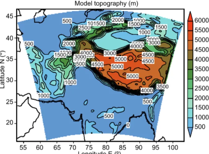
the Biosphere-Atmosphere Transfer Scheme (BATS) (Dickinson et al., 1993) and the Community Land Model (CLM) (Oleson et al., 2008) schemes. For this study, the span of the model domain is 18-45º N, 60-95º E. The model domain and the orography
shown in Figure 1 cover all parts of northwest India. A model grid with horizontal resolution of
30 × 30 km is selected to conduct the simulation experiments. As can be seen from the figure, the maximum height of the Himalayas represented at
this resolution is about 5500 m. Most of the sharp gradient in the orography of the Himalayas gets smoothed out due to the resolution chosen for the model. Sinha et al. (2013) carried out a detailed
study on the role of representation of orography in
the RegCM3 simulations.A brief on model config
-uration used in this study is also given in Table I.
In this study, two sets of numerical experiments
are carried out with different land surface models,
BATS and CLM.
The BATS land surface parameterization scheme
is used to describe the role of soil moisture and
vegetation in the model. It calculates the exchanges
of momentum, energy, and water vapor associated with surface-atmosphere interactions. It has one vegetation layer, a surface soil layer, a snow layer and 20 vegetation types. The prognostic equations for the soil layer temperatures are solved by using a
generalized force-restore method (Dickinson et al.,
1993). The CLM (Oleson et al., 2008) contains one
vegetation layer with a canopy
photosynthesis-con-ductance model, 10 unevenly spaced soil layers, five
snow layers with an additional representation of trace snow, and 24 vegetation types. In this scheme, for each layer temperature, ice water and liquid water are
solved explicitly. The CLM uses a mosaic approach
for capturing land surface heterogeneity within a climate model at each grid cell. The main advantage
of the CLM over BATS is that in the former, a higher
number of soil layers and vegetation fractions are included. The CLM has the ability to include sub-grid “tiles” with separate water and energy balance conducted for each tile. This approach enables the
representation of various surface parameters (e.g., surface temperature, precipitation, fluxes, etc.) in a better way compared to BATS (Steiner et al., 2005).
A brief comparison of these two land surface param-eterization schemes is provided in Table II.
1000 1000 1000 1000 1500 1500 1000 500 500 500 500
Latitude N (º)
500 0 4000 4500 4500 3500 2500 4500 3500 5000 5000 2000 5000 4000 3000 3000 2000 1500 1500 2000 101500 4000 3000 30003000 45
Model topography (m)
40 35 30 25 6000 5500 5000 4500 3500 2500 1500 500 4000 3000 2000 1000 20
55 60 65 70 75 80 85 90 95 100
Longitude E (º)
3. Simulation specifics and verification method -ology
Seasonal (winter) precipitation anomalies over
the Indian areas of the Western Himalayan region
have been computed using 33 years (1975-2008) of
observed precipitation data from the India
Meteoro-logical Department (IMD) (Rajeevan et al., 2006).
For the present study, extreme (excess or deficit)
precipitation seasons are considered on the basis of precipitation anomalydepartures by one standard deviation or more from its mean. Therefore, within
these 33 years, there are three years in the category of excess precipitation (1990-1991, 1994-1995, 1997-1998, hereafter referred to as excess years); Table I. Configuration of the RegCM4 used in the present study.
Dynamics Hydrostatic
Main prognostic variables u,v t, q and p
Model domain 18-45º N, 60-95º E; res. = 30 km
Map projection Lambert conformal mapping Vertical coordinate Terrain-following sigma coordinate
Total: 18 sigma levels (five levels in PBL)
Cumulus parameterization Grell with Fritch & Chappell closure
Land surface models Biosphere-Atmosphere Transfer Scheme (BATS) and Community Land Model (CLM)
Radiation parameterization NCAR/CCM3 radiation scheme
PBL parameterization Holtslag
Table II. A brief comparison between two land surface parameterization schemes (i.e., BATS and CLM).
Category BATS CLM
Land cover/vegetation
classes 20 vegetation types 24 vegetation types
Surface representation One vegetation layer, a surface soil layer,
a snow layer One vegetation layer with a canopy photosynthesis-conductance model, 10 unevenly spaced soil layers, five snow layers with an additional representation of trace snow
Soil temperatures
calculation Uses a two-layer force-restore model Soil temperature is calculated explicitly by a 10-layer soil model Treatment of vegetation
canopy Treats all vegetationwithin the canopy in the same manner
The canopy is divided into sunlit and shaded fractions as a function of LAI
Calculation of stomatal conductance and photosynthesis rate
No individual calculation is made for sunlit and shaded fractions. It does not compute photosynthetic rates
Stomatal conductance is calculated for sunlit and shaded fractions. Calculation of photosynthetic rates is done in this scheme
Treatment of heat and
roughness length Heat and water vapor roughness lengths are constant Updates these values over bare soil and snow with values from the stability functions Albedo treatment Uses prescribed values for vegetation
albedo for both short- and longwave components
Uses a modified two stream approach that reduces the complexity of a full two-stream albedo
three years in the category of deficit precipitation (1996-1997, 2000-1901, 2004-1905, hereafter referred to as deficit years), and three years in the category of normal precipitation (1988-1989, 1993-1994, 2003-2004, hereafter referred to as normal years). In the present study, these years are consid
-ered to conduct the numerical experiments. Com -posite analyses have been carried out by computing
the difference between excess minus normal and deficit minus normal precipitation years.
The RegCM model has been integrated from
November 1 to February 28 (February 29 during the leap year) for each winter season. In this study, model integration output for the first month (i.e., November)
is not analyzed as it is considered the model spin up
time. For each year (excess, deficit and normal), the
RegCM model is integrated twice with two different
LSPS; first, coupled with BATS and then coupled with
CLM, keeping unchanged all the other parameters of the model. Initial and lateral boundary conditions
(LBCs) for the model integration are provided by the
National Centers for Environmental
Prediction-De-partment of Energy (NCEP-DOE) reanalysis II to drive the RegCM model, and the LBCs are updated
every 6 h. The prescribed sea surface temperature in the model is the National Oceanic and Atmospheric
Administration Optimum Interpolation SST (NOAA-OI-SST-v. 2) at a 1 × 1º resolution). The geophysical
parameters are from the United States Geophysical
Survey (USGS) at a 10’ resolution). The model-sim
-ulated results are validated with the IMD gridded (1 × 1º) observed precipitation and surface air temperature (hereafter simply referred to as temperature) data sets.
For comparison of the model data with observations, model simulated results are interpolated bilinearly to the grid points of the observed data.
Statistical analysis such as spatial correlation
coefficient (CC), root mean square error (RMSE), probability of detection (POD), equitable threat score (ETS), etc., have been carried out between model and
IMD data sets. The POD indicates what fraction of the observed “yes” events was correctly forecasted.
It is defined as,
POD = H H+ M (1)
where H and M are hits and misses for each category, respectively. POD ranges from 0 to 1 with POD = 1 indicating perfect skill in prediction (i.e., M = 0).
ETS is a skill metric generally used for yes/no forecasting (Gilbert, 1884; Wilks, 1995); it is de
-fined as:
ETS = (H + MH + – FH – λ H , where
λ)
Hλ = (H + M) (TM + F)
(2)
and M, H and F are the number of misses, hits and false alarms, respectively, for each category. Hits due to random chance are denoted by Hλand T is the total
number of events. ETS varies from –0.33 to 1 with
ETS = 0 indicating no skill and ETS = 1 indicating perfect skill in prediction. Student’s t-test is used for
statistical significance of the anomaly CC, where the critical value of CC is 0.27 at a 90% confidence level (CL).
4. Results and discussion
The composite analyses of observed gridded tem-perature and precipitation during the winter season
for excess, deficit and normal precipitation years
are presented in Figure 2. It is clearly seen from the
figure that temperature is comparatively cooler during the excess years as compared to normal and deficit
years over Jammu and Kashmir. It is also seen that
the seasonal mean temperature is warmer by 1-2 ºC during deficit years than in excess years over the
Western Himalayan region. The range of seasonal
mean precipitation during excess years is about 4.5
to 6.5 mm day–1 with a maximum of 6.5 mm day–1
over Jammu and Kashmir, whereas during deficit
years the seasonal precipitation range is about 1.5 to 2.5 mm day–1, with a maximum of 2.5 mm day–1 over the same region. Therefore, it is noticed that
excess precipitation years are comparatively cooler than deficit precipitation years over the Indian part
of the Western Himalayan region. In the following three sub-sections, the results obtained from the simulation of RegCM model with two different LSPS are analyzed.
4.1 Spatial distribution of surface air temperature
It was noticed that the model is able to reproduce the mean temperature distribution over the northwest
India for the composite excess, composite deficit
and composite normal yearsreasonably well when
either of the land surface schemes (BATS or CLM) are used (figure not shown). However, the simulated
temperature in terms of distribution and magnitude is
better in the CLM experiment than in the BATS when
results are compared against the observed surface temperature data sets.
In order to understand the variation of seasonal av-erage winter temperature in distinct years, composite
differences between excess and normal years, as well as between deficit and normal years are computed and shown in Figure 3. It can be seen from the figure
that temperature is lower in the observations and in
both RegCM simulation experiments in the excess
years as compared to normal years. The left panel in
Figure 3 shows that the RegCM model with BATS simulates a warmer surface by 1-2 ºC as compared to the CLM in the difference between composite excess
and composite normal precipitation years. On the other hand, it is found that the area with cooler tem-perature is located more over the Western Himalaya
Latitude N (º)
Excess
(a) (Comp_Temp) (d) (Comp_Precip)
(b) (e)
Excess
Deficit Deficit
(c) Normal (f) Normal
40
35
30
25
20
Latitude N (º)
40
30 6.5
5.5
4.5
3.5
2.5
1.5
0.5 26
22
18
14
10
6
2 35
30
25
20
Latitude N (º)
40
35
30
25
20
65 70 75 80 85 90 95
Longitude E (º) 65 70 75Longitude E (º)80 85 90 95 Fig. 2. Seasonal (DJF) average of IMD gridded temperature (in ºC) and precipitation
(in mm day–1) for composite excess (a, d), composite deficit (b, e) and composite
in the CLM than in the BATS. It can also be noticed
that the magnitude and distribution of temperature
differences between deficit and normal years with the CLM scheme is better than with the BATS when compared with the observed patterns (Fig. 3, right panel). The analysis reveals an improvement of 10-20% in the predictions of seasonal mean winter temperature with the use of CLM over BATS. So,
the results suggest that the model-simulated mean
as well as the variation in temperature (in terms of spatial distribution and magnitude) during the nine
distinct yearsare better represented with the use of
CLM as compared to BATS.
4.2 Spatial distribution of precipitation
The response of the BATS and CLM schemes in the RegCM model is examined in terms of precipitation
simulations in the nine distinct yearsdescribed earlier. Results indicate that the model is able to represent the seasonal mean precipitation distribution for
the composites of excess, deficit and normal years reasonably well with both land surface schemes (figure
(c) CLM (f) CLM
Latitude N (º)
40
35
30
25
20
Latitude N (º)
IMD
(a) (Excess-Normal) (d) (Deficit-Normal)
(b) (e)
IMD
BATS BATS
40
35
30
25
20
Latitude N (º)
40
3
2
1 2.5
1.5
0.5
–0.5 –1
–2
–3 0
–1.5
–2.5 35
30
25
20
65 70 75 80 85 90 95
not shown). However, in terms of distribution and
intensity the model-simulated precipitation is closer to observations with the use of the CLM scheme. To
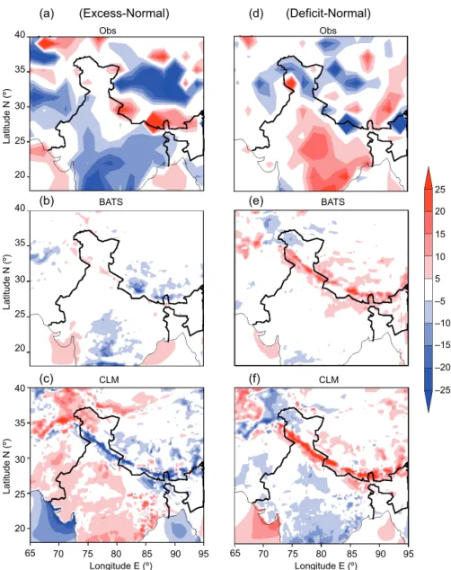
understand the RegCM model efficiency in simulating
precipitation during the nine distinct years, the
sea-sonal mean (DJF) composite precipitation differences between excess and normal years, as well as between deficit and normal years, are computed.Precipitation differences are shown in Figure 4. In the precipitation
difference between excess and composite normal years
(Fig. 4, left panel), it is seen that the representation
of precipitation in terms of intensity and distribution
is better with CLM than with BATS scheme when
compared to observed differences. The precipitation
differences between deficit and normal years (Fig. 4, right panel) are captured well in both LSPS (CLM and BATS) over northwest India, however, the variation
in precipitation is closer to the observations with the
CLM scheme than with BATS. The qualitative de -scription of seasonal precipitation suggests that the
efficiency of the RegCM model is higher with the CLM scheme than with BATS.
The area average of monthly as well as seasonal composite precipitation obtained from the IMD
(c) CLM (f) CLM
Latitude N (º)
40
35
30
25
20
Latitude N (º)
IMD
(a) (Excess-Normal) (d) (Deficit-Normal)
(b) (e)
IMD
BATS BATS
40
35
30
25
20
Latitude N (º)
40
1
0.6
0.2 0.8
0.4
0
–0.4 –0.6 –0.8 –0.2
–1 35
30
25
20
65 70 75 80 85 90 95
Longitude E (º) 65 70 75Longitude E (º)80 85 90 95
Fig. 4. Seasonal (DJF) difference of average precipitation (composite excess – compos
observations and the RegCM (with BATS and CLM) simulations were computed and are exhibited in
Figure 5, which shows that the area-averaged pre-cipitation is underestimated in both LSPS during
all of the years (composite of excess, composite of deficit and composite of normal years, respective
-ly) at monthly as well as seasonal scale. However,
the RegCM simulations with CLM are closer to observations. An improvement in the precipitation
magnitude by about 15-25% is noticed with the CLM scheme over BATS in the seasonal mean
simulations. It may be noticed that the improvement varies from year to year. During all the months
and seasons, the efficiency of the RegCM model is higher when run with CLM instead of BATS, though
the rate of improvement is higher in January than in other months. The better simulation of precipitation
with CLM as compared to BATS may be due to the
inclusion of more number of soil layers and a better
representation of the vegetation cover in the former, as described below.
The vegetation cover over the region of interest
as used by both LSPS (BATS and CLM) is shown
in Figure 6. It can be seen from the diagram that vegetation cover in the RegCM-CLM simulations has a greater spatial coverage over the Indian part of
the Western Himalaya than the RegCM-BATS. This
increased vegetation cover in the RegCM-CLM en-hances precipitation as found in Zheng et al. (2002).
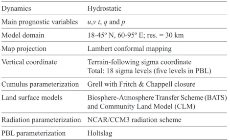
Soil moisture from the NCEP-DOE reanalysis II
and the RegCM simulations (with BATS/CLM LSPS) are shown in Figure 7 for the composites of excess and normal years, and deficit and normal
precipitation years.Observations show positive soil moisture over northern India, which is well brought
out by both LSPS. However, the spatial extent is lower in the RegCM-BATS simulation for the com
-posite of excess minus normal years.In the case of 0
1 2 3 4 5 6
(a)
0 1 2 3
December January February DJF
December January February DJF
December January February DJF
(b)
BATS CLM IMD
0 1 2 3 4 5 (c)
mm day–1
mm day–1
mm day–1
Fig. 5. Monthly and seasonal average precipitation (mm day–1) from IMD gridded
precipitation, and RegCM4 model simulation with BATS and CLM, for (a) com
the composite difference between deficit and normal
precipitation years,the spatial extent and intensity
is closer to observations with the RegCM-CLM as
compared to the RegCM-BATS simulation. This dif -ference in model simulation is due to the dif-ference in soil descriptions and moisture representations between these two LSPS. Therefore, the better representation of soil moisture may be the reason for a better representation of precipitation in the RegCM-CLM simulation.
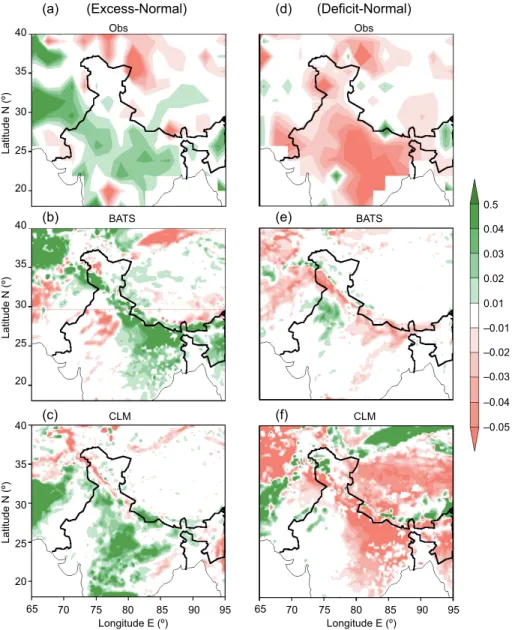
Sensible heat fluxes from the NCEP-DOE re
-analysis II and the RegCM simulations (with BATS/ CLM LSPS) are depicted in Figure 8 for composites of excess minus normal and deficit minus normal
precipitation years.The composite analysis between
excess minus normal precipitation years indicates that both LSPS show almost similar spatial extents
of precipitation over the eastern parts of Jammu and Kashmir. However, over the western part of Jammu and Kashmir, the RegCM-CLM simulation produces
more wet zones as compared to the RegCM-BATS
simulation. In the case of composite differences
between deficit and normal precipitation years, sim -ulations with both land surface schemes are mostly similar.
4.3 Statistical evaluation of precipitation
The performance of the RegCM model with the BATS
and CLM land surface schemes has been evaluated
by computing various statistical skill scores. Some important evaluation strategies consisted in esti-mating the RMSE and the CC, between others. The model skill scores were estimated against observed gridded precipitation data from the IMD over the Indian part of the Western Himalaya. The model re-sults are bi-linearly interpolated to the grid points of the IMD observed data for statistical evaluation. The RMSE and spatial CC are calculated for both sets of
runs using CLM and BATS (Table III). It can be seen that the CC is statistically significant (the threshold value is 0.27 at a 90% confidence level) in the pre -cipitation simulation with the CLM scheme during
excess, deficit and normal precipitation years. The CC is higher in the CLM experiment (0.39, 0.35 and 0.37, respectively) than in the BATS experiment for
all the years in which simulations were carried out within this study. The RMSE values of the RegCM model are lower when the CLM scheme is used
in comparison with BATS. This suggests that the
spatial distribution of precipitation and its intensity are simulated better in the RegCM with the CLM
scheme than with BATS.
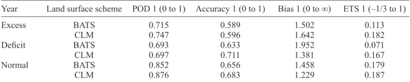
Several other skill metrics, such as POD, accu-racy, ETS, and bias have been estimated for the dis-tinct precipitation years and presented in Table IV. When the observed precipitation is higher than or equal to 1 mm day–1, that day is considered as a wet day. It can be seen from the statistical Fig. 6. Vegetation cover in (a) BATS and (b) CLM land surface schemes.
24 23 22 21 20 19 18 17 16 15 14 13 12 10 9 8 7 6 5 4 3 2
1 11
40 (a) BATS
35
30
25
20
Latitude N (º)
(b) CLM
40
35
30
25
20
65 70 75 80 85 90 95
Latitude N (º)
Longitude E (º)
65 70 75 80 85 90 95
analysis that POD values are higher in the CLM
experiment (0.75, 0.70 and 0.88 for the excess, deficit and normal years, respectively) than in the BATS experiment for all the three distinct years.
It is also found that the number of wet days
simu-lated in the CLM experiment is closer to observa -tions. Furthermore, the accuracy of precipitation
simulations is higher with CLM than with BATS
over the Western Himalaya. The computed model bias indicates that the precipitation intensity and distribution is better represented with the CLM
(bias is closer to 1). However, the model-simulated
(c) CLM (f) CLM
Latitude N (º)
40
35
30
25
20
Latitude N (º)
Obs
(a) (Excess-Normal) (d) (Deficit-Normal)
(b) (e)
Obs
BATS BATS
40
35
30
25
20
Latitude N (º)
40
35
30
25
20
65 70 75 80 85 90 95
Longitude E (º) 65 70 75Longitude E (º)80 85 90 95 0.5
0.04
0.03
0.02
0.01
–0.01
–0.02
–0.03
–0.04
–0.05
Fig. 7. Seasonal (DJF) soil moisture (kg/kg) difference (composite excess – composite normal and composite deficit – composite normal precipitation year) obtained from observed data (a, d) and RegCM4 model simulation with BATS (b, e) and CLM (c, f).
precipitation is underestimated with respect to observations in both schemes. Table IV indicates that ETS is higher in the CLM simulations during all the years, which indicates that precipitation events are better represented with the CLM land surface scheme.
Thus, the statistical analysis (forecast errors and skill scores) also reveals that the RegCM model with
the CLM parameterization scheme performs better
in simulating precipitation for extreme years with
reasonable accuracy over the Western Himalayan
5. Conclusion
In the present study we compared two different land surface parameterization schemes within the
Reg-CM, i.e. BATS and CLM, to simulate nine distinct
winter precipitation years over the Western Himala-ya. During the winter months, a notable difference
between the BATS and CLM experiments is ob -served in the simulation of temperature and amount of precipitation. The performance of the RegCM with both LSPS is reasonable in reproducing the mean features of seasonal temperature and precipitation, however the skill of the model is higher with the
Fig. 8. Seasonal (DJF) sensible heat flux (W m–2) difference (composite excess – com
-posite normal and com-posite deficit – com-posite normal precipitation year) obtained from observed (a, d) and RegCM4 model simulation with BATS (b, e) and CLM (c, f).
(c) CLM (f) CLM
Latitude N (º)
40
35
30
25
20
Latitude N (º)
Obs
(a) (Excess-Normal) (d) (Deficit-Normal)
(b) (e)
Obs
BATS BATS
40
35
30
25
20
Latitude N (º)
40
35
30
25
20
65 70 75 80 85 90 95
Longitude E (º) 65 70 75Longitude E (º)80 85 90 95 25
20
15
10
5
–5
–10
–15
–20
–25
Table III. RMSE and CC for excess, deficit and normal
precipitation years.
Excess Deficit Normal
RMSE BATS 3.448 1.587 2.778
CLM 3.312 1.385 2.529
CC BATS 0.359 0.313 0.351
CLM 0.385 0.352 0.374
Table IV. Skill score for excess, deficit and normal precipitation years for the > 1 mm rainfall category.
Year Land surface scheme POD 1 (0 to 1) Accuracy 1 (0 to 1) Bias 1 (0 to ∞) ETS 1 (–1/3 to 1)
Excess BATS 0.715 0.589 1.502 0.113
CLM 0.747 0.596 1.642 0.182
Deficit BATS 0.693 0.633 1.952 0.071
CLM 0.697 0.711 1.381 0.167
Normal BATS 0.852 0.656 1.458 0.179
CLM 0.876 0.683 1.229 0.187
CLM scheme. Furthermore, temperature and
precip-itation during extreme winter seasons are also better captured with the CLM scheme than with BATS
when compared to observations. As mentioned earlier, most of the sharp gradient in the orography of the Himalayas gets smoothed due to the resolu-tion chosen for the model. Similarly, the surface
characteristics (soil type, soil wetness, vegetation cover, etc.) are not properly represented in the mod -el due to the chosen resolution, as there is a sharp gradient in these parameters over the Himalayan region. This study suggests that even at this
reso-lution, the RegCM model with CLM and BATS is
able to reproduce some of the salient features of the
distinct years examined.
Forecast errors and skill scores indicate that the performance of the RegCM model is better with the
CLM scheme rather than with BATS. Moreover, im
-provements by about 10-20% in temperature and 15-25% in precipitation predictions are observed with the use of the CLM scheme in comparison with BATS.
In sum, the study indicates that the RegCM model with the CLM scheme can be more informative in simulating wintertime temperature and precipitation over the Western Himalayan region.
Acknowledgments
The authors acknowledge the support of the Snow
and Avalanche Study Establishment (SASE) for
carrying out this study. The RegCM4 installed at IIT Delhi was developed at the Abdus Salam ICTP, Trieste, Italy and is duly acknowledged. The au-thors also acknowledge the India Meteorological Department for providing valuable data sets for the accomplishment of this work. The authors also duly acknowledge the NCEP for reanalysis II data and the NOAA for optimum interpolated SST, v. 2
(NOAA_OI_SST_V2) data provided by the NOAA/ OAR/ESRL PSD, Boulder, Colorado, USA, from
their web site at http://www.esrl.noaa.gov/psd/. Au -thors also wish to thank two anonymous reviewers for their constructive suggestions that improved the
manuscript significantly.
References
Dickinson R. E., A. Henderson-Sellers and P. J. Kennedy,
1993. Biosphere-atmosphere transfer scheme (BATS)
version 1e as coupled to the NCAR Community
Climate Model. NCAR Technical Note NCAR/TN-387+STR, 72 pp., doi:10.5065/D67W6959.
Dickinson R. E., 1995. Land-atmosphere interaction. Rev. Geophys. 33, 917-922.
Ding Y., J. Zhang and Z. Zhao, 1998. An improved
land-surface processes model and its simulation ex
-periment. 2. Land-surface process model (LPM-ZD) and its coupled simulation experiment with regional
climate model. Acta. Meteorol. Sin. 56, 385-400.
Dutta S. K., S. Das, S. C. Kar, U. C. Mohanty and P. C. Joshi, 2009. Impact of vegetation on the simulation of seasonal monsoon rainfall over the Indian sub-continent using a regional model. J. Earth Syst. Sci.
118, 413-440.
Fritsch J. M. and C. F. Chappell, 1980. Numerical pre
-diction of convectively driven mesoscale pressure systems, part 1: Convective parameterization. J. Atmos. Sci. 37, 1722-1733.
Gilbert G. K., 1884. Finley’s tornado predictions. Am.
Meteorol. J. 1, 166-172.
Giorgi F. and G. T. Bates, 1989. On the climatological skill
of a regional model over complex terrain. Mon. Wea.
Rev. 117, 2325-2347.
Grell G. A., 1993. Prognostic evaluation of assumptions
used by cumulus parameterization. Mon. Wea. Rev.
121, 764-787.
Grell G. A., J. Dudhia and D. R. Stauffer, 1994. Description
Henderson-Sellers A. and R. E. Dickinson, 1993. Atmo-spheric-land surface fluxes. John Wiley and Sons, pp.
387-405.
Holtslag A. A. M., E. I. F. de Bruijn and H. L. Pan, 1999.
A high resolution air mass transformation model for short-range weather forecasting. Mon. Wea. Rev. 118, 1561-1575.
Kar S. C., P. Mali and A. Routray, 2014. Impact of land surface processes on the South Asian monsoon sim-ulations using WRF modeling system. Pure Appl. Geophys. 171, 2461-2484.
Kiehl J. T., J. J. Hack, G. B. Bonan, B. A. Boville, B. P. Briegleb, D. L. Williamson and P. J. Rasch, 1996.
Description of the NCAR Community Climate Model
(CCM3). NCAR Tech. Note NCAR/TN- 420+STR,
152 pp.
Oleson K. W., G. Y. Niu, Z. L. Yang, D. M. Lawrence, P. E. Thornton, P. J. Lawrence, R. Stockli, R. E.
Dickin-son, G. B. Bonan, S. Levis, A. Dai and T. Qian, 2008.
Improvements to the Community Land Model and their impact on the hydrological cycle. J. Geophys. Res. 113, 1021-1026.
Pal J. S., F. Giorgi, X. Bi, N. Elguindi, F. Solmon, X. Gao,
S. A. Rauscher, R. Francisco, A. Zakey, J. Winter, M.
Ashfaq, F. Syed, S. Faisal. J. L. Bell, N. S. Diffenbaugh,
J. Karmacharaya, A. Konare, D. Martinez, R. P. Da Rocha, L. C. Sloan and A. L. Steiner, 2007. Regional climate modeling for the developing world: The ICTP
RegCM3 and RegCNET. Bull. Amer. Meteor. Soc. 88,
1395-1409.
Pielke R. A. and R. Avissar, 1990. Influence of landscape
structure on local and regional climate. Landscape Ecol. 4, 133-155.
Pielke R. A., D. D. S. Niyogi, T. N. Chase and J. L.
East-man, 2003. A new perspective on climate change and
variability: A focus of India. Proc. Indian Nat. Acad. Sci. 69, 585-602.
Rajeevan M., J. Bhate, J. Kale and B. Lal, 2006. High
resolution daily gridded rainfall data for the Indian region: analysis of break and active monsoon spells. Curr. Sci. 91, 296-306.
Singh A. P., U. C. Mohanty, P. Sinha and M. Mandal,
2007. Influence of different land surface processes on
Indian summer monsoon circulation. Nat. Hazards
42, 423-438.
Sinha P., U. C. Mohanty, S. C. Kar and S. Kumari, 2014. Role of the Himalayan orography in simulation of the
Indian summer monsoon using RegCM3. Pure Appl.
Geophys. 171, 1385-1407.
Steiner A. L., J. S. Pal, F. Giorgi, R. E. Dickinson and W. L. Chameides, 2005. A coupling of common land
model (CLM0) to a regional climate model (RegCM).
Theor. Appl. Climatol. 82, 225-243.
Tiwari P. R., S. C. Kar, U. C. Mohanty, S. Dey, P. Sinha, P.V.S. Raju and M. S. Shekhar, 2014. Dynamical downscaling approach for wintertime seasonal scale simulation over the Western Himalayas. Acta Geo-physica. 62, 930-952.
Wilks, D.S., 1995. Statistical methods in the atmospheric sciences. Academic Press, San Diego, 467 pp.
Zheng Y., Yongfu Qian, Manqian Miao, Ge Yu, Yushou