Key words: Consolidation Analysis, Biot’s Formulation, Plasticity in Soils Mechanics, Finite

CONSOLIDATION IN SATURATED POROUS MEDIA.

IMPLEMENTATION

AND NUMERICAL PROBLEMS.

Héctor A. Di Rado *, Armando M. Awruch ^ and Pablo A. Beneyto *

*

Applied Mechanics Department. Northeast National University (U.N.N.E.)

Las Heras 727

3500 Resistencia, Chaco, Argentina.

e-mail: [email protected], web page: http://ing.unne.edu.ar/

^

Graduate Program in Civil Engineering Federal University of Rio Grande do Sul

Av. Osvaldo Aranha 99 90035-190 Porto Alegre, RS, Brazil.

e-mail: [email protected]

Key words: Consolidation Analysis, Biot’s Formulation, Plasticity in Soils Mechanics, Finite

Elements.

Abstract :The main aim of this Paper is to present a two dimensional mathematical model

based on Biot's theory (1955) [3],[4], which allows to analyse the total stresses equilibrium (effective + pore) and the strain compatibility during the consolidation process by coupling the effects of stress and flow. It is taken into account geometric and physical non linear behaviour. For the latter, an elastoplastic or, alternatively, a viscoplastic model based on the critical state theory, with some modifications [6],[16]_{, is considered.}

Another objective of this work, is to present some of the implementations difficulties and numerical problems that has been detected during the analysis. The influence of the failure function form and parameters like permeability, soil grain and water compressibility, is presented. Furthermore, the behaviour of soil mass under initial stresses effects, is checked.

INTRODUCTION

The solution of load displacement problems in clays is , generally ‘coupled’, since the applied loads set up the excess pore pressure which is dissipated by seepage flow. This physical phenomenon is usually called “Consolidation”.

Consolidation problems are matter of big deal in clay type or compacted soils with generally low permeability. Such is the case of many cities located at the northeast area of Argentine in which this kind of soil is widely found, creating uncertainties by the time of planning direct big foundations. It is also quite common to find, at the mentioned cities and its influence area, high tenors of humidity (nearby to saturation) due to the small depth of the groundwater table. This fact has motivated us to pay a special attention to saturated soils.

Considering the fact that the geographical situation of many local cities made possible periodical flooding, there is another kind of construction also greatly used at the mentioned region :The earth dams. Many of the design problems in these kind of structure are very similar to that appearing in direct foundations, which allow us to suppose that most of the tools presented here, could be overturned in dams projects.

Even if the principal aim of this Paper is to obtain an accurate stress-strain relationship as well as a consistent stress path in a saturated soil mass submitted to loads, there is another, but not less important, goal to bring out : the numerical problems due to the consideration of certain parameters like soil grain an water compressibility included in those matrices that govern the fluid motion in the pores.

The influence of many other parameters will also be analysed along the present work. The problem is solved by means of the Finite Element Method.

Concluding this preliminary remarks, it must be indicated that our final goal is to expand the present mathematical model to cover those cases in which the two - phase nature (soil-water) is not enough to describe the real phenomenon, and air should be incorporated to form an unsaturated three - phase system.

GENERAL FORMULATION

The principal feature in saturated porous media is the two - phase nature defined by the fact that soil grains are surrounded by a fluid (generally water) that originates pressure on the solid phase.

The five basics concepts that gives support to consolidation theory are:

a) Effective stress principle.

b) Constitutive law for the solid skeleton. c) Equilibrium of the whole porous media. d) Fluid motion equation.

Effective stress principle.

It is usual, for geological materials, to split total stress rate into effective stress rate and pore stress rate, giving

σ σ σ

~ ~ m p~ ~

• • • •

= ′− −

Pr

(1)

where the point over each letter indicates time derivatives (rate), σ•

~ is the Total stress rate ,

′

•

σ

~ is the Effective stress rate , p

•

is the Pore pressure rate and σ

~

•Pr

represents the stress rate due to strains rate in soil grains generated by pore pressure.

For this analysis, p is positive and σ ′

~ is negative for compression effects. Constitutive law for the solid skeleton.

The effective stress rate is related to strain rate by the expression :

′ =  −   _ = • • • • • σ ε ε σ ε ~ ~ ~ ~ IN ~ pr ~ ~ pr

D and D (2)

where ε

~ IN

•

indicates the infinitesimal inelastic (either viscoplastic or elastoplastic ) strain rate vector. y ε

~ pr

•

is the infinitesimal strain rate vector due to pore pressure. The expressions for the former and the latter, respectively, are :

(

)

=  +        = 1

2 , 12 3, , (3)

ε ~ pr ~ _s m p 3k • •

= − or ε• δ

(

)

•

= − =

ij _ij i j

pr

s

p

3k , 1 2 3, , (4)

where δ_ij is Kroenecker delta., u_iare displacement components and ks is the bulk modulus of

soil grains.

It can be considered that isotropic volumetric strain rate is due to hydrostatic pore pressure. Combining (1), (2) and (4), it is obtained:

σ ε ε ε σ σ α σ σ ~ ~ • • • ′ • • • • • • =  −   _ − − = ′− −         = ′− • •

D D mp m m m Dm

3k mp mp

~ ~ ~ IN ~ ~ pr ~ ~ ~ T ~ ~ T ~ ~

s ~ ~ ~

~ pr

6 74 48 678

1

where α denotes the Biot coefficient and it is defined by α = −1 m D m 9k ~

T ~ ~

s

. Expression (5), stands for the actual constitutive law.

Equilibrium of the whole porous media.

The equilibrium may be assured by using the well-known soil equilibrium equations :

(

)

∂σ ∂

ij

j i

x i j

• •

+b =0 , =1 2 3, , en Ω (6.a)

where bi

•

are components of the mass rate forces vector in directions of coordinates

(

)

x_i i =12, ,3 and Ω is the entire domain.

Nevertheless, there is another widely used expression that also represents equilibrium in addition to some boundary conditions, the so-called virtual displacement principle (VDP) given by:

δ ε σ δ δ

σ

~ T

~ ~

T

~ ~

T ~

• • • • • •

∫

∫

∫

Ω Ω Γ

(6.b) Including in (6.b), the constitutive equations (5) and displacement-specific strain relationships (3) , a useful expression for VDP is obtained:

δ ε ε δ ε δ δ

σ

~ T

~ EP ~ ~

T ~

T ~

~ T

~ ~

s ~ ~

T

~ ~

T ~

D m m m D m

3k mp b

• • • • • • • •

∫

∫

∫

∫



  



 

 = +

dΩ dΩ u dΩ u t dΓ

Ω Ω Ω Γ

1

3 (6.c)

where an elastoplastic stress-strain relationship was used. Initial and essential boundary conditions (not presented here) should be applied.

Fluid motion equation.

The equation of the fluid motion in the pores is given by Darcy’s law and it is defined by :

(

)

v z

~= − ∇~k~ γ +p (7)

In the expression written above, ”v

~” is the vector containing fluid velocity components,

“k

~” the soil permeability tensor, “γ ” is the fluid specific weight, “z” is geodesic high with

regards to a reference system and “∇

~ ” is the gradient vector. Fluid mass conservation.

∇ − =•

~ T

~

v Ψ 0 (8)

where “Ψ• ” is the rate of fluid accumulation. Many factors influence “Ψ• ”. Some of them are :

a) The rate of fluid accumulation due to bulk specific strains :

Ψ•1= −ε•vol= − ε•

~ T

~

m (9)

b) The rate of fluid accumulation due to volume changes of the soil grains because of pore pressure changes, yielding:

( )

( )

Ψ• •

•

= − = − −

2 1 n 1 n p

k

vol pr

s

ε (10)

where “k_s” is grain compressibility modulus.

c) The rate of fluid accumulation due to fluid compressibility, giving:

Ψ•3= − n •

k_f p (11)

where “k_f” is fluid compressibility modulus.

d) The rate of fluid accumulation due to soil grain compressibility produced by changes in

′−

• • σ σ

~ ~

pr

. The average hydrostatic compression developed in this case is given by :

Ψ• • • = ′− 4 3 m k ~ T ~ s ( ~ )

σ σpr

(12)

Regarding expression (5), leads to

Ψ• =  • •− •   _ +         4 1 3 1 3

k_sm D~ k mp

T

~ ~ ~

IN

s ~

ε ε (13)

Substituting (9), (10), (11) and (13) into (8), provided (7), a convenient form of the conservation equation is reached:

( )

k _k m D m p k p + m

m D

3k k

m D

3k

s f _s ~

T ~ ~ ~ T ~ ~ ~ T ~ T ~

s ~ ~

T ~ ~ ~ T ~ ~ IN s

ε ( * )γ z ε (14)

Finally, (6.c) together with (14) is a coupled system of equation with u ~

•

and p as primary unknowns, provided that the constitutive model (5) is verified.

THE ELASTOPLASTIC MODEL.

A critical state theory and the model proposed by Zienkiewicz et. al. [16] and lightly modified here, was used for stress-strain relationship. The failure surface is defined by :

(

)

(

)

F ′ = + _c



   



   

− =

p , q, p 2

q p * tg

p

2

θ

φ 2 1 0 0 (15)

where, p′ =-J₁/3 ( average pressure), q=

( )

J with J₁ and J₂being the first and second effective stress tensor invariants, (2 )

0

p_c −a is the initial pre-consolidation pressure, p p += ′ a

(with a= c_tgφ ),c is the cohesion and φ is the internal fiction angle given by

(

)

tg sen

3 cos -sen sen

φ φ

θ φ θ

=3 and finally, θ is the third invariant.

An isotropic strain Hardening rule was used for the failure surface evolution. Thus, considering an exponential law for the hardening parameter p_c

0 (widely used in soil

analysis), it gives:

p p_c

0 vol pl

c₀ = 0 e(−χ ε ) (16)

where ε_volpl _{is volumetric plastic strain and χ is giving by}

χ β λ

= +

−

K 1 e₀

(17) In the expression written in above, “e0” is the initial void ratio, λ and K are constants

determined by the oedometer test and β is an authors proposal that allows a better adjustment of (16) to different soils and may be obtained by laboratory experiments. However, a value approximately equal to the initial p_c

0, can be used.

The so-called plastic modulus used in the elastoplastic matrix expression, is given by:

A

p p

p _q

(p +a) tg

= − = −



 

  

  

    1

2 1

0 0

0

2

Λ ∂

∂ χ φ

F d

c c

c

(18)

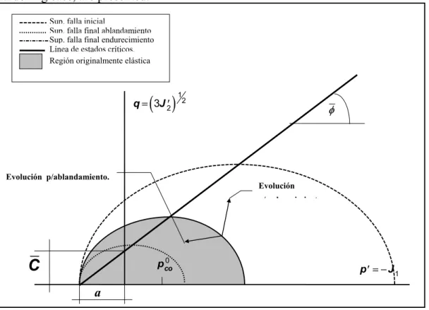
It is usual to present plastic models for soils in a “p-q” plot instead of presenting it in a Haigh - Westergaard space. Therefore for a better comprehension of the plastic model, in the following figure (figure 1) the initial and the final failure surface, either for softening and hardening case, are presented.

Figure 1 - Critical state model adopted.

FINITE ELEMENT APPLICATION

Here, unknowns “u

~” and “p” are interpolated between their nodal values using 8-nodes

Serendipity Shape functions N

~

u _{for the former and 4-nodes Serendipity Shape function N} ~ p

for the latter (further explanations will be given later on), yielding:

u u u

e e

u e e u e u

~ ~ ~ ~

p

~ ~ ~ ~ ~

T

~ ~ ~

p

~ ~

T

~ ~

N U p N p B U U N p N p U B

T T

T T

• • • • • • • • • •

= ( ); = ( ) ; ε= ( );δ =δ ( ) ; δ = δ ; δ ε =δ ( ) (19)

The application of the finite element procedure, leads expression (6.b) to the following form :

K U L p P

~ ~ ~ _~ ~

( )e •( )e₋ ( )e •( )e ₌•( )e ₍₂₀₎

where

Sup. falla inicial

Sup. falla final ablandamiento Sup. falla final endurecimiento Línea de estados críticos.

( )

q= 3J₂′ 12

′ = −

p J₁ p_co0

Región originalmente elástica

φ

C

a

K B D B L B m Dm

9k mN P N b N

~ ~ ~ EP ~ ~ ~

~ T

~ ~

s ~ ~

p ~ ~ ~ ~ ~ T (e) T (e) T (e) T ( ) _; ( ) _; ( ) ( )

e u u_d e u _d e u _d u _{t d}

e = = −         = + ∫ ∫ • ∫ • ∫ • Ω Ω Ω Γ

Ω 1 Ω Ω Γ

σ

(21)

being Ω(e) the element domain (e) and Γ(e) the boundary element portion under surface loads

t ~ .

By application of Galerkin method with a weighting functionδp to expression (14), integrating by parts and using (19), leads to:

S p L U H p P

~ _~ ~ T ~ ~ _~ ~ 1 ( ) ( ) ( ) ( ) ( ) ( ) ( )

e e e e e e

e

• • •

+ + = − (22)

where

S N sN H N k N

~ p T ~ p ~ ; ( ) ( ) 1 e ij e i l lm j m e d

x x d

= _∫ =_∫ Ω Ω Ω ∂ Ω ∂ ∂ ∂

and (23)

P N k N m D

3k N ~ p ~ p ~ T ~ s ~ IN ~ p T T • = _∫ + _∫ • + _∫ ( ) ( ) / ) ( ) e

l lm m

n x

z

x d d v d

e e ve ∂ ∂ ∂γ ∂ ε Ω Ω Γ Ω Ω Ω with

( )

s 1- n k

n

k _k m D m

s f _s ~

T ~ ~

= + − 1

3 2 and

(

)

v z

n v ni i vn

n = −k_n p + =

∂ γ

∂ ;

Putting together (20) and (22), the coupled governing equations are obtained. They can be written in a matrix form as follows :

K L L S U p 0 0 0 H U p P -P ~ ~ ~ ~ ~ ~ ~ ~ ~ ~ ~ ~ ~ ~ T ( ) ( ) ( ) ( ) ( ) ( ) ( ) ( ) ( ) ( ) e e e e e e e e e e −                       +                =             • • • • 1 (24)

Solving the time integration problem using the α parameter method (with 0≤ ≤α 1) and an incremental scheme, (24) becomes :

K L

L S H

U p H U p P P ~ ~ ~ ~ ~ ~ ~ ~ ~ ~ ~ ~ T ( ) ( ) ( ) ( ) ( ) ( ) ( ) ( ) ( ) ( ) ( ) ( ) e e

e e e

e e e e e t e e t t − − −_ + _                   =              +         1 0 0 0 α∆ ∆ ∆ ∆ ∆

∆ (25)

In equation (25), the sign in the last equation was changed in order to avoid a non symmetric system.

Values for coming time, are obtained with the following expressions:

U U U

~t t ~ ~

e t

e e

+∆ = +∆

( ) ( ) ( ) _{and p p p}

~t t ~ ~

e t e e + = + ∆ ∆

The incremental expression (25) should be applied to the whole domain and adding the essential boundary condition, a non lineal set of equation is achieved. Once the system is solved, expression (26) is applied until convergence.

INTRODUCTION OF GEOMETRIC NON LINEARITY EFFECTS

Considering geometric non linearity effects, expression (20) must be modified introducing the geometric stiffness matrix and the unbalanced force vector.

Taking into account that an objective measure of stress rate must be used, the Jaumann[12] stress rate tensor was adopted for this work . Components of this tensor are defined:

σJ_ij =σ_ij−σikwkj−σ jkwki

• • •

(

)

where σ•_ij are components of the Cauchy stress rate tensor and wij

•

are the components of the spin rate tensor.

Virtual work principle at stage t = t+∆t, but referring to stage t , may be expressed :

δ∆ σ ∆σ Ω δ∆ ∆ Ω δ∆ ∆ Γ

Ω Ω Γ

e J d u b b d u t t d

t t

t t T

~ T

T T

(

~+ ~) = ~ (~ + ~) + ~ (~ + ~)

•

∫

∫

∫

where e

~ is the finite Lagrangian strain tensor,σ~ contains components of the Cauchy tensor at

stage t, (

~ ~)

σ+∆σ•J stands for stresses at t+∆t (with∆σ

~

•J

containing components of the Jaumann stress rate tensor increment), b b

t

~ +∆~ y ~tt+∆~t are loads at t+∆t.

Splitting e

~

•

in its linear part ε

~

•

and non linear part η

~

•

and substituting in (28), leads to:

δε σ δ σ δ η σ δ δ δε σ

~ T

~ T

~ _~

T

~ T

~ T

~ T

~

∆ Ω ∆η Ω ∆ Ω ∆ Ω ∆ Γ Ω

Ω ~ Ω Ω ~ Ω ~ ∆ Γ ~ ∆ Ω

• •

+ +

+ + = + −

∫ Jd ∫ _td ∫ Jd ∫ u b_{t t}d ∫ u t_{t t}d ∫ _td

t t t t t t

(29)

Neglecting the third integral in the left hand side of (29) and providing that

∆σ ∆ε ∆

~ ~ EP ~ ~

~ ~ s

D D

3k p

•

= − −

  



   J

m m (30)

where e

~ ~

• •

≅ε was considered, the obtained equation is similar to (20) but the geometric matrix and the unbalanced force vector must be added to the left and to the right hand side respectively . The incremental finite element equation at element level is given by :

(K( ) K ( )) U( ) L( ) p( ) P( )

~ ~ ~ ~ _~ ~

e G

e e e e e

+ ∆ − ∆ =∆ (31)

K

~

~G e

G T

t G

B B d

=

∫

~ σ ~

Ω

Ω (32)

where B G

~ contains derivatives of the displacement interpolation functions.

Cauchy stresses at each gauss point, are obtained using the following expression:

σ σ ε σ σ

~ ~

T T

~ + ~ )

t+∆t= t+(D~*∆~ + ∆ω *~ ∆ω*~ t (33)

In expression (33),( ~ ~)

σ+∆σ•J was replaced by ( ~ ~)

σ+∆σ and the computed stresses will be used in next time step.

APPLICATIONS

Strip Footing.

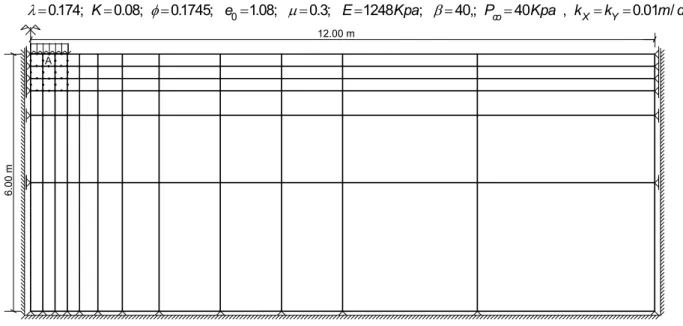
As a first example, a strip footing of 12m width is analyzed. The footing is assumed to be smooth, flexible an impervious. The soil has been assumed to be homogenous, weightless and isotropic. Seepage is allowed only on the load free top surface. The remaining borders are consider impervious. Complete geometric characteristics are shown in figure 2. Principal soil constants are :

λ=0174. ; K=0 08. ; φ=01745. ; e₀=108. ; µ=0 3. ; E=1248Kpa; β=40,; P_co=40Kpa , k_X=k_Y=0 01. m dia/

Fig. 2 Strip footing. Finite element model.

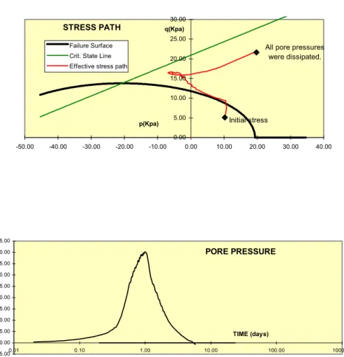
The following plots present in first place the effective stress path and afterwards, the evolution of pore pressures along time steps :

k_S=8500Kpa k; _F =8500Kpa c; =11Kpa, non-isotropic initial stresses.

STRESS PATH

Initial stress

All pore pressures were dissipated.

0.00 5.00 10.00 15.00 20.00 25.00 30.00

-50.00 -40.00 -30.00 -20.00 -10.00 0.00 10.00 20.00 30.00 40.00

p(Kpa) q(Kpa)

Failure Surface Crit. State Line Effective stress path

PORE PRESSURE

-5.00 0.00 5.00 10.00 15.00 20.00 25.00 30.00 35.00 40.00 45.00

0.01 0.10 1.00 10.00 100.00 1000.00

TIME (days)

Fig. 3 Stress path and pore pressure.

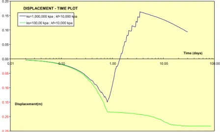
DISPLACEMENT - TIME PLOT

0.25 0.20 0.15 0.10 0.05

0.00 0.05 0.10 0.15 0.20

0.01 0.10 1.00 10.00 100.00 Time (days)

Displacement(m)

ks=1,000,000 kpa ; kf=10,000 kpa ks=100,00 kpa ; kf=10,000 kpa

Fig. 4 Displacement- time under the load.

Earth dams.

The main characteristics of the earth dams commonly found in the area are : a) The small dimensions. b) The homogeneous of its constitution.

The final example presented here, is referred to the following earth dam (figure5). Drainage is allowed on the upper surface, upstream and downstream. The gauss points number three and one belonging to elements A and B respectively, were chosen for relating all drafts. The remaining data is :

A B

Fig. 5 Earth Dam. Finite element model.

λ φ µ β

γ

= =

= =

= =

= =

= =

= =

0174 0 08

0 108

0 3 450

10 15

0 01 10000

0

3

. ; . ;

;

. ; ;

,;

. /

.3; .

,

,

=1.6 /

K e

E Kpa

P Kpa

k k m dia

k k Kpa

KN m co

X Y

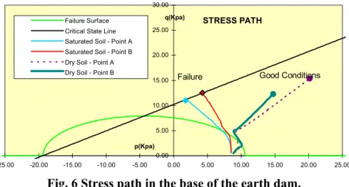
For the mentioned dam, only gravity loads was considered. Two situation were taken into account : 1) The use of dry soil. 2) The use of saturated soil.

In the following plot, the stress paths for both cases were analyzed :

STRESS PATH

Failure Good Conditions

0.00 5.00 10.00 15.00 20.00 25.00 30.00

-25.00 -20.00 -15.00 -10.00 -5.00 0.00 5.00 10.00 15.00 20.00 25.00

p(Kpa) q(Kpa)

Failure Surface Critical State Line Saturated Soil - Point A Saturated Soil - Point B Dry Soil - Point A Dry Soil - Point B

Fig. 6 Stress path in the base of the earth dam.

Clearly, the effect of developed pore pressures provokes the dam failure at early stages when water is present, with the difference from the dry case in which all load is supported.

COEFFICIENTS ANALYSIS.

Soil and water compressibility analysis.

The problem presented here is quite similar to that of incompressible elasticity where numerical instabilities are regarded. The comparison can be carried out considering that in both cases there is a well conditioned matrix, an ill conditioned matrix and a coupling matrix. By inspection of equation (25), K

~ correspond to the first one, S~1+ H~



 α∆t  correspond to the

second and L

~ denotes the coupling matrix.

The numerical problems are owed to the fact that quantities in S

~ 1are divided by fluid and

grain compressibility, commonly very high values, and H

~ includes soil permeability

coefficients, which have low values when clays are under consideration. Therefore

S H

~1+ ~



 α∆t is close to a null matrix.

Likewise for incompressible elasticity and to avoid numerical troubles, two main cautions must be taken into account :

a) The number of displacements unknowns(U

~) must be greater than pore pressure

ones(p

~). The reason lies in the different order of each unknown, considering that “p~”

is, indeed, a stress what is similar to say a “U

b) Both compressibility coefficients should be taken as penalty parameters rather than use their real values and reduced integration should be used.

The first condition was accomplished considering different order of the shape function for displacements and for pore pressure. For the former an eight nodes quadrilateral element was used while for the latter, a four nodes one was chosen.

In order to achieve the last condition, the modification consists in minimizing of coefficient values allowing the increase of S

~ 1elements, and consequently all system is better

conditioned.

However, it is necessary to be aware that an arbitrary modifications like this, should distort the whole physical phenomenon and this fact can not be allowed.

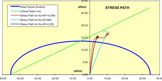
As showed in figure(7), the lower the compressibility coefficients are taken, the lower values in pore pressure are obtained. Under such circumstances, a greater load transference form water and soil grains to soil skeleton is noticed producing an increase in effective stress and in volumetric strains.

Whenever the above outlined process is fitted to reality, a correct penalty parameter adoption was carried out.

Concluding, it can be recommended to use values for penalty parameters nearby ten times and one hundred times the value of the initial elasticity module for the fluid and grain compressibility respectively. However, a tantamount value for both coefficients may be used in some special occasions.

STRESS PATH

0.00 5.00 10.00 15.00 20.00 25.00 30.00

-50.00 -40.00 -30.00 -20.00 -10.00 0.00 10.00 20.00 30.00 40.00

p(Kpa) q(Kpa)

Initial Failure Surface Critical State Line Stress Path for Ks=Kf=10,000 Stress Path for Ks=Kf=850 Stress Path for Ks=Kf=4,250

Figure 7 - Influence of different compressibility over stress paths.

Failure function shape analysis.

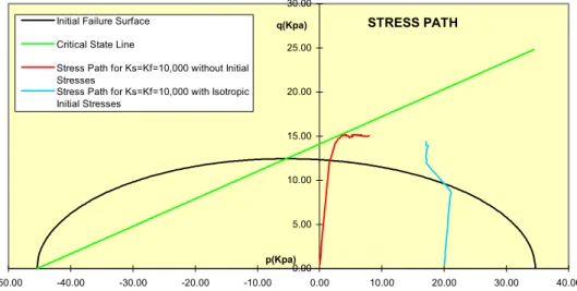
a) When stress path goes through the yield surface to places where the normal to this curve(taken as the plastic strain vector) has a great horizontal component, what means great volumetric plastic strain (see Figure 1), the stress path beyond the elastic zone trends to the left. The justification lies in the fact that the higher volumetric plastic strains, the higher pore pressure and thereby, less effective stresses will be developed. This kind of stress path is obtained from laboratory testes using normally consolidated samples with a little drainage. Taking into account that a stress path as described above is achieved only when the initial stress level is close to initial pre-consolidation stress (almost normally consolidated) and considering that in clay type soils water flux is hardly allowed, an accordance between numerical simulation and laboratory practice, was found.

b) On the opposite, whether the stress path induces a small horizontal component in plastic strain vector and therefore a scant amount of volumetric plastic strains, it trends to the right (increasing in “p’ ”). This behavior is typically found in over-consolidated samples. Likewise the previous case and based on a similar analysis, another concordance in simulation an laboratory testing was proved.

Figure (8) can be inspected for further comprehension. It must be stood out that the coincidences elsewhere outlined should be analyzed between the frame of discrepancy that this kind of comparison generates itself.

STRESS PATH

0.00 5.00 10.00 15.00 20.00 25.00 30.00

-50.00 -40.00 -30.00 -20.00 -10.00 0.00 10.00 20.00 30.00 40.00

p(Kpa) q(Kpa)

Initial Failure Surface

Critical State Line

Stress Path for Ks=Kf=10,000 without Initial Stresses

Stress Path for Ks=Kf=10,000 with Isotropic Initial Stresses

Figure 8- Influence of failure function form over stress path.

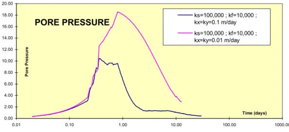
Permeability coefficient analysis.

without any problem and, furthermore, improvement in that stability was detected.

PORE PRESSURE

0.00 2.00 4.00 6.00 8.00 10.00 12.00 14.00 16.00 18.00 20.00

0.01 0.10 1.00 10.00 100.00 1000.00

Time (days)

Pore Pressure

ks=100,000 ; kf=10,000 ; kx=ky=0.1 m/day ks=100,000 ; kf=10,000 ; kx=ky=0.01 m/day

Figure 9- Influence of permeability coefficients.

As can be expected, the figure (9) is useful to confirm that, the higher permeability coefficients are, the lower pore pressures developed.

CONCLUDING REMARKS

• A two dimensional coupled model with physical and geometric non linearity for consolidation analysis in low permeability clay-type saturated soil, has been presented and some of the numerical troubles due to some of the involved parameters, have been regarded.

• Adaptability of the flow function was improved by inclusion of the parameter β, which makes possible to use oedometer and triaxial testes for calibrating purposes. It should be remarked that the lower is the value of β, the closer to perfect plasticity.

• To simulate pore pressure dissipation across time, the load must be kept constant and the equation system is solved applying flux load only.

• Numerical troubles due to the small quantities of the components in flux and mass matrices, should be overcame by taking fluid and grain compressibility as penalty parameters. This means that the correct value should be chosen regardless the real one but always preserving the physical phenomenon. Thus, these quantities were found to be nearby ten times and a hundred times the initial elasticity module for the fluid and grain compressibility respectively.

• When initial stresses are under consideration, the model shows less instabilities, but different penalty coefficients should be considered in comparison with the case where initial stresses are neglected.

• Higher values of permeability coefficients favor water flux and thereby a pore pressure dissipation. The numerical difficulties were also appeased with the increasing of these coefficients.

ACKNOWLEDGMENTS

REFERENCES

[1] ATKINSON J.H. and BRANSBY P.L., The mechanics of soils. An introduction to critical state soil mechanics. University Series in Civil Engineering. Mc. Graw. Hill (1978)

[2] BATHE, K. J and CIMENTO, A. P. Some Practical Procedures for the solution of Nonlinear Finite Element Equations. Comp. Meth. in Appl. Mech. and Engng, V22, pp. 59-85 (1984).

[3] BIOT, M. A. General theory of three - dimensional consolidation. J. of Applied Physics, V. 12, pp. 155 - 164 (1941).

[4] BIOT, M. A. Theory of deformation of a porous viscoelastic anisotropic solid, J. of Applied Physics, V. 27, pp. 459 - 467 (1956).

[5] CARTER,P; BOOKER, J.R. and SMALL, J.C. The analysis of finite elasto-plastic consolidation. Int. J. Num. Analyt. Meth. in Geomech, V.3, pp. 107-129 (1979).

[6] DI RADO H. A. & AWRUCH, A.M. Un modelo elastoplástico con grandes deformaciones para suelos cohesivos basado en la teoría de los estados críticos. COPAINGE .Tomo 1. Pp.37 a 47. (1997)

[7] GOLUB, G. H. and VAN LOAN, C. F. Matrix Compretatirs , John Hopkins University Press, Baltimore (1984).

[8] HILL, R. The Mathematical Theory of Plasticity. Oxford University Pren, UK, 1950. [9] KIM, C. S..; LEE, T. S.; ADVANI, S. H. and LEE, J. H. Hygro thermomechanical evaluation of porous media under finite deformation; Part II; Model validation and field simulation. Int. J. for Numer. Meth. in Engng., V.36, pp. 161- 179 (1993).

[10] LEWIS, R. W. and SCHREFLER, B, A, The Finite Element Method in the Deformation and Consolidation of Porous Media. J. Wiley & Sons, N. Y, 1987.

[11] MALVERN, L. E. Introduction to the Mechanics of a Continuum Medium, Prentice Hall, Englewood Cliffs, nj (1969).

[12] NAYAK, G. C. and ZIENKIEWICZ, O. C. Elastic - Plastic stress analysis. A generation of various constitutive relations including strain softening. Int. J. for Numer. Meth. in Engng.., V.5, pp 113- 135 (1972).

[13] OWEN, D. R. J. and HINTON, E. Finite Elements in Plasticity; Theory and Practice. Pineridge Press Limited, Swansea, U. K, 1980.

[14] VILADKAR, M. N.; NOORZAET, J. and GODBOLE, P. N. Convenient forms of yield criteria in elasto-plastic analysis of geological materials Comp. & Structures, V.54, pp. 327- 337 (1995).

[15] ZIENKIEWICZ, C. C.; HUMPHESON, C. and LEWIS, R. W. A unified approach to soil mechanics problems (including plasticity and visco-plasticity). In: Finite Elements in Geomechanics (Ed. by Gudehus), pp 151-177 J. Wiley & Sons, London (1977).