TítuloAn optimal quantity tax path in a dynamic setting
35
0
0
Texto completo
(2) N. Nawaz / European Journal of Government and Economics 6(2), 191-225. maximizing the consumer welfare subject to the condition that a competitive equilibrium holds in each time period. In Judd (1985), the government taxes capital income net of depreciation at a proportional rate, which is assumed to be constant. Chamley (1986) analyzes the optimal tax on capital income in general equilibrium models of the second best. Deaton and Stern (1986) show that optimal commodity taxes for an economy with many households should be at a uniform proportional rate under certain conditions. Cremer and Gahvari (1993) incorporate tax evasion into Ramsey’s optimal taxation problem. Cremer and Gahvari (1995) prove that optimal taxation requires a mix of differential commodity taxes and a uniform lump-sum tax. Naito (1999) shows that imposing a non-uniform commodity tax can Pareto-improve welfare even under nonlinear income taxation if the production side of an economy is taken into the consideration. Saez (2002) shows that a small tax on a given commodity is desirable if high-income earners have a relatively higher taste for this commodity or if consumption of this commodity increases with leisure. The quantity taxes are currently more popular in the environmental economics literature, e.g. Nordhaus (1993) proposes an optimal carbon tax (tax per ton of carbon). Chari, Christiano and Kehoe (1994) deal with the labor and capital income taxes instead of a quantity tax as in our model. Ekins (1996) takes into account the secondary benefits of Carbon dioxide abatement for an optimal carbon tax. Coleman (2000) derives the optimal dynamic taxation of consumption, income from labor, and income from capital, and estimates the welfare gain that the US could attain by switching from its current income tax policy to an optimal dynamic tax policy. Pizer (2002) explores the possibility of a hybrid permit system and a dynamic optimal policy path in order to accommodate growth and not because of the adjustment over time to equalize the marginal benefit and cost. It is implicitly assumed that the marginal cost equals the marginal benefit in each time-period. Following Ramsey, the existing literature on optimal quantity taxation only compares the pre and the post-tax market equilibriums in order to account for the efficiency losses. However, when the government imposes a quantity tax on the consumer, the buyer’s price jumps to the pre-tax equilibrium price plus the amount of the tax, and the supply and the demand of the taxed commodity then adjust over time to bring the new post-tax market equilibrium. The existing literature does not take into account the efficiency losses during the adjustment process while computing the optimal quantity taxes. This paper derives an optimal quantity tax path in a dynamic setting minimizing the efficiency losses (output and/ or consumption lost) during the dynamic adjustment process as well as the post-tax market equilibrium. The remainder of this paper is organized as follows: Section 2 explains how the individual components of the market system are joined together to form a dynamic market model. Section 3 provides the solution of the model with a quantity tax imposed. Section 4 derives an optimal commodity tax path minimizing the efficiency losses subject to a tax revenue target in a specific time-period. Section 5 summarizes the findings and concludes. The appendix presents mathematical details.. 192.
(3) N. Nawaz / European Journal of Government and Economics 6(2), 191-225. 2. The model. Let’s assume that there is a perfectly competitive market of a single homogeneous commodity in equilibrium (so our starting point is when the market is already in equilibrium). There are four types of infinitely-lived agents: a representative -or a unit mass of- producer (that produces a good, and demand labor and capital), a middleman (who buys the good from firms to sell to consumers, and possibly accumulating inventories), a representative –or a unit mass of– consumer (who buys the good, accumulates capital by investing and supplies labor inelastically), and a government. The role of middleman is motivated by the real world scenario where the producer and the consumer seldom directly meet for a transaction to take place. The existence of retailers, wholesalers, financial institutions, educational institutions and the hospitals reflect the presence of middlemen between producers and consumers in most of the economic activity going on. The producer produces the goods and supplies those to the middleman, who keeps an inventory of the goods and sells those to the consumer at the market price. In the model, the middleman plays a key role, as she sets the selling price 𝑝𝑝 by maximizing the difference between the revenue for selling goods to consumers and the costs of inventories. The buying price paid to the producer is 𝛼𝛼 𝑝𝑝 with 𝛼𝛼 < 1, and the producer is a price taker.. The price adjustment mechanism is based on the fact that when a shock leads the market out. of equilibrium, the buyers’ and sellers’ decisions are not coordinated at the current prices. An example can illustrate the working of this market. Consider that the market is initially in equilibrium. The middleman has an equilibrium stock of inventory. Then, an exogenous demand contraction will increase the stock of inventory, due to firms’ output could not match with the –now lower– units demanded by the consumer at the current price. This excess of supply is accumulated in inventory held by the middleman. The middleman will decrease the price so that the producer will find optimal to produce a lower level of output. A new equilibrium with a lower price and a lower level of output is then reached. The equilibrium is defined as follows: (i) The producer and the middleman maximize their profits and the consumer maximizes her utility subject to the constraints they face (mentioned in their individual dynamic optimization problems in Section 2). (ii) The quantity supplied by the producer equals the quantity consumed by the consumer (and hence the inventory does not change when the market is in equilibrium). The conditions for the existence of the equilibrium (Routh–Hurwitz stability criterion, which provides a necessary and sufficient condition for the stability of a linear dynamical system) have been mentioned in Section 3. As the set-up is for a perfectly competitive market, therefore, the middleman who sells the goods to the consumer at the market price is a price taker when the market is in equilibrium. When the market is out of equilibrium, the middleman can change the price along the dynamic adjustment path until the new equilibrium arrives, where again the middleman becomes a price taker. The government announces and imposes a commodity tax at the same time (the expectations of the agents will be taken into account in a future research project when the dates 193.
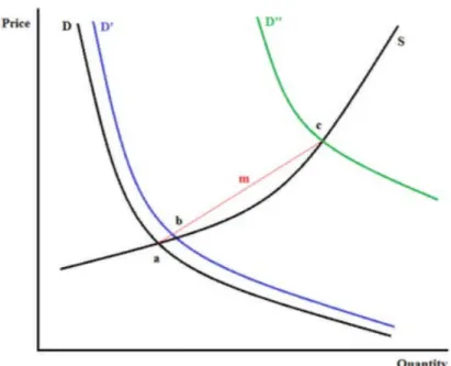
(4) N. Nawaz / European Journal of Government and Economics 6(2), 191-225. of announcement and implementation of the tax are different). When a commodity/ quantity tax is imposed, the market does not suddenly jump to the post-tax market equilibrium, rather the price adjusts over time to bring the new equilibrium. This adjustment process involves endogenous decision making (in their own interest) by all the agents in the market, i.e. consumer, producer and the middleman as follows: Suppose there is a producer in a market who produces a perishable good and sells it to a middleman who further sells it to a consumer living in a community. The producer and the middleman sell a quantity exactly equal to the quantity the producer produces in each time period, and the market stays in equilibrium. If the government announces and imposes a commodity tax on the buyer, which decreases the demand of this product, some of the production sold to the middleman will remain unsold to the consumer and be wasted by the end of the time period in which the tax was imposed. Assuming that the producer and the middleman can change the production and the price respectively, immediately, had they known the exact pattern of new demand, they would immediately pick the quantity (by the producer) and the price (by the middleman) to maximize their profits and clear the market without wasting the production. However, they lack this information, so the middleman decreases the price based on her best guess about the new demand (based on the quantity of the unsold production), driving the market close to the new equilibrium. At the lower price, the producer produces a lower quantity than before. If in the following time period, his production sold to the middleman is fully sold out to the consumer, he will know that the new equilibrium has arrived, however, if a part of his production still remains unsold, the middleman will reduce the price further (and the producer, the production accordingly) to bring the market closer to the new equilibrium. The market will eventually settle at the new equilibrium after some efficiency loss. The resources wasted by the imposition of the tax are those that went into the unsold production in each timeperiod during the adjustment process. A new equilibrium with a deadweight loss due to commodity taxation is finally arrived at. The total efficiency loss because of commodity taxation is the loss during the adjustment process plus the loss in the final equilibrium. For the mathematical treatment, the objective of each of the three market agents is maximized through the first order conditions of their objective functions and to capture the collective result of their individual actions, the equations representing their individual actions are solved simultaneously. For simplification, we assume that after the imposition of the quantity tax, the new equilibrium is not too far from the initial equilibrium. This assumption makes the linearization of supply and demand curves quite reasonable; see Figure 1 (the time axis is not shown). Linearization seems to be a good approximation when we move from point a to b, whereas it is not a good approximation when we move from point a to c. For modeling the movement of the market from point a to c, we need to model a non-linear dynamical system (which is not covered under the scope of this paper).. 194.
(5) N. Nawaz / European Journal of Government and Economics 6(2), 191-225. Figure 1: When is Linearity a Reasonable Assumption?. 2.1 Middleman. The middleman purchases goods from the producer and sells those to the consumer for profit. As happens in the real world, the middleman does not buy and sell exactly the same quantity at all points in time, thus he holds an inventory of the goods purchased to be sold subsequently. Inventory is an intermediary stage between supply and demand which reflects the quantum of difference between supply and demand of the goods in the market. If the inventory remains the same, it implies that demand and supply rates are the same. An increase or decrease in inventory implies a change in supply, demand or both at different rates. Figure 2 helps to understand the link between inventory, supply, demand and prices. When the supply curve shifts to the right (while demand remains the same), the inventory in the market increases at the initial price, and the new equilibrium brings the price down. Similarly, when the demand curve shifts to the right (while supply remains constant), the inventory depletes from the market at the previous price and the new equilibrium brings the price up. This shows that there is an inverse relationship between an inventory change and a price change (all else the same). If both the supply and demand curves shift by the same magnitude such that the inventory does not change, then price will also remain the same. Inventory unifies the supply and demand shocks in the sense that they are both affecting the same factor, i.e. inventory and are basically the faces of the same coin. Therefore each kind of shock is in fact just an inventory shock. From the above mentioned discussion, we have seen that there is an inverse relationship between an inventory change and a price change.. 195.
(6) N. Nawaz / European Journal of Government and Economics 6(2), 191-225. Figure 2: Movement of Price with Inventory.. Now let’s discuss the mechanism which brings about such a change. Consider a market of homogeneous goods where the middlemen, such as whole sellers, retailers, etc. hold inventories, incur some cost for holding those, and sell products to the consumers to make profits. The cost is a positive function of the size of an inventory, i.e. a larger inventory costs more to hold as compared to a smaller inventory. In the absence of an exogenous shock, if the supply and demand rates are equal then the system is in equilibrium and the price does not vary with time. Suppose that a technological advancement decreases the marginal cost of production and increases the supply rate, whereas the demand rate remains the same. As the demand and supply rates are no longer equal, therefore the difference will appear somewhere in the economy in the form of piled up inventories. As the production flows from the producer to the consumer through the middleman, therefore it is reasonable to assume that the middleman will be holding the net difference (Explanation: The piled up inventories can also be in the form of producers’ inventories of finished goods, which does not change the key point that a difference of supply and demand rates directly affect the inventories in the economy). The economy will not be able to sustain this situation indefinitely, and the middlemen will have to think of some means of getting rid of piled up inventories. The only resort they have is to decrease the price which brings the demand up along the demand curve. 196.
(7) N. Nawaz / European Journal of Government and Economics 6(2), 191-225. In a perfectly competitive market, the price will eventually come down to equalize the new marginal cost, however the adjustment path depends on how the middlemen react to the change in their inventories. Notice that the marginal cost of production has decreased but the marginal cost of holding an extra unit of inventory for the middleman has increased. This is an intuitive explanation which is theoretically consistent with the demand, supply, utility and profit maximization by a consumer and a producer respectively. In the real world, we see examples of this behavior of middlemen, e.g. as consumers, we enjoy the end of year sales, offers such as buy one get one free, gift offers if you buy above a certain quantity threshold, etc. For a mathematical treatment, we need to consider the profit maximization problem of the middleman as follows. 2.1.1 Short-run problem. Let’s first consider the short-run problem of the middleman as follows (the middleman’s objective is myopic rather than doing dynamic optimization. In a discrete analog, this is a one period analysis, which is presented for an intuitive purpose as an anticipation of the -more complicateddynamic problem in section 2.1.2).. Π = pq ( p ) − ς (m( p, e)),. [1]. where. Π = profit, p = market price, q ( p ) = quantity sold at price p,. m = inventory (total number of goods held by the middleman), e = other factors which influence inventory other than the market price including the middleman’s purchase price from the producer,. ς (m( p, e)) = cost as a function of inventory (increasing in inventory). The first order condition (with respect to price) is as follows: .. .. .. p q ( p ) + q ( p ) − ς (m( p, e)) m1 ( p, e) = 0,. [2]. The middleman has an incentive to change the price only during the adjustment process and will incur losses by deviating from the price (equal to the marginal cost) when the market is in equilibrium. During the adjustment process, the demand does not equal the supply and the market drifts toward the new equilibrium (however, the price cannot move automatically and it is reasonable to assume that some economic agent moves the price in her own benefit), therefore a price change by the middleman in the direction of bringing the new equilibrium is not against the market forces, so he does not lose business by changing price on the adjustment path unlike when the market is in equilibrium and where the middleman faces an infinitely elastic demand as 197.
(8) N. Nawaz / European Journal of Government and Economics 6(2), 191-225. follows: .. .. .. p q ( p ) + q ( p ) = ς (m( p, e)) m1 ( p, e), .. . 1 m1 ( p, e) p 1 + = ς (m( p, e)) . , demandelasticity q( p) .. q( p) demandelasticity = p . q( p) The right hand side of the above expression is the marginal cost which equals the price when the middleman faces an infinitely elastic demand. Suppose that as a result of a supply shock, the marginal cost of production decreases, and the supply curve shifts downwards. Now the competitive market is out of equilibrium as the demand does not equal the supply at the previous equilibrium price. The price must eventually decrease to bring the new equilibrium, however, the price will not jump to equalize the demand and supply, and rather the middleman will continue charging a price higher than the new marginal cost until the market forces make him realize that the supply has increased and he needs to lower the price to satisfy the profit maximizing condition. The similar is the case of a reverse supply shock, where the price must eventually increase to bring the new equilibrium. In this case, the middleman will continue charging a price lower than the marginal cost until the market forces make him increase the price, in which case it is the consumer who is the short term beneficiary. Again, the consumer will be paying a price less than the marginal cost only during the adjustment process and only until the middleman increases the price. The equilibrium price is equal to the marginal cost of production plus the marginal cost of storage (i.e. the total marginal cost) in the absence of any kind of a tax, so neither does the middleman earn any economic rent, nor does the consumer benefit by paying a price less than the marginal cost when the competitive market is in equilibrium. For the mathematical treatment, suppose that as a result of a supply shock (while demand remains the same) such as a technological advancement which reduces the marginal cost of production and increases the supply by the producers, if the middleman wants to hold an extra . .. unit of inventory, his marginal cost of holding an extra unit, i.e.. ς (m( p, e)). m1 ( p, e) .. , is higher at. q( p) .. the previous price, because the term. ς (m( p, e)). is higher at the previous price. This might be. on account of higher storage charges because of increased demand of warehouses, godowns, .. etc. after increased supply in the market. The second term, i.e.. m1 ( p, e) .. is a function of price,. q( p) and is the same as before as the price has not changed yet (we are assuming that the middleman’s purchase price is the same as before as the producer is a price taker during the 198.
(9) N. Nawaz / European Journal of Government and Economics 6(2), 191-225. adjustment process as well and always charges a fixed fraction of the market price to the middleman). A discrete analog of this scenario is that the middleman maximizes profits in each time period without considering the future time periods, and in each time period he takes the purchase price from the producer as given and only chooses the sale price. This implies that on the previous price, now the middleman faces . . . ∂Π = p q ( p ) + q ( p ) − ς (m( p, e)) m1 ( p, e) < 0, ∂p. [3]. which means that the middleman must decrease the price to hold an extra unit of inventory to satisfy the profit maximizing condition after the supply shock. Please notice that in this static scenario, the short term gains accrued from the decreased marginal cost of production will be reaped by the producer, as his marginal cost has decreased but he charges the same price to the middleman until the middleman changes the price. If we plot together various profit maximizing combinations of inventories and the respective prices chosen by a middleman, we will get a downward sloping inventory curve with the price on the y -axis and the inventory on the. x -axis.. This is analogous to the concept of supply and demand curves for the profit maximizing producers and the utility maximizing consumers respectively.. 2.1.2 Dynamic problem. Now let’s consider the dynamic problem of the middleman. In a dynamic setting, the middleman maximizes the present discounted value of the future stream of profits, and his present value at time zero is as follows: ∞. V (0) = ∫[ pq ( p ) − ς (m( p, e))]e − rt dt ,. [4]. 0. where r denotes the discount rate, p (t ) is the control variable and m(t ) the state variable. The maximization problem can be written as ∞. Max V (0) = ∫[ pq ( p ) − ς (m( p, e))]e − rt dt , { p ( t )}. 0. subject to the constraints .. .. .. .. .. .. m(t ) = m1 ( p (t ), e( p (t ), z )) p (t ) + m2 ( p (t ), e( p (t ), z )) e1 ( p (t ), z ) p (t ). (state. describing how the state variable changes with time; z are exogenous factors),. m(0) = ms (initial condition), m(t ) ≥ 0 (non-negativity constraint on state variable), m(∞) free (terminal condition). 199. equation,.
(10) N. Nawaz / European Journal of Government and Economics 6(2), 191-225. The current-value Hamiltonian for this case is . . . ~ m ( p(t ), e( p(t ), z )) + m2 ( p(t ), e( p (t ), z )) ∗ [5] . H = p(t ) q( p(t )) − ς ( m( p(t ), e( p(t ), z ))) + µ (t ) p(t ) 1 . ( ( ), ) e p t z 1 . The maximizing conditions are as follows:. ~ ∂H ~ = 0, (i ) p (t ) maximizes H for all t : ∂p ~ . ∂H , (ii ) µ − rµ = − ∂m ~ . ∗ ∂H (this just gives back the state equation), (iii ) m = ∂µ ∗. (iv) lim µ (t )m(t )e − rt = 0 (the transversality condition). t →∞. The first two conditions are as follows:. ~ ∂H = 0, ∂p. [6]. ~ ∂H . µ − rµ = − = ς (m( p(t ), e( p (t ), z ))). ∂m. [7]. and .. ~ ∂H boils down to the When the market is in equilibrium, p (t ) = 0, and the expression ∂p .. following (see appendix): . . . . 1 m1 ( p (t ), e( p (t ), z )) m2 ( p (t ), e( p (t ), z )) e1 ( p (t ), z ) ( ), ))) ( ), ( = ( ( + z e p t m p t p (t ) 1 + ς , . . demandelasticity q ( p (t )) q ( p (t )) . whiche suggests that the price equals the marginal cost (the right hand side of the above expression is the marginal cost in a dynamic setting, which is different from that in a static problem on account of the fact that in a dynamic setting the middleman also takes into account the impact of price chosen on his purchase price from the producer) when the demand is infinitely elastic. Now suppose that as a result of a supply shock, if the middleman wants to hold an extra unit of inventory, then the marginal cost of holding an extra unit is higher because the term .. ς (m( p(t ), e( p(t ), z ))). is higher at the previous price at that point in time. The term in 200.
(11) N. Nawaz / European Journal of Government and Economics 6(2), 191-225. parentheses. in. the. .. expression. .. m1 ( p (t ), e( p (t ), z )) .. +. of. the. marginal. cost,. i.e.. .. m2 ( p (t ), e( p (t ), z )) e1 ( p (t ), z ) .. q ( p (t )). is a function of price and is the same at. q ( p (t )). the previous price. This implies that on the previous price, now the middleman faces. ~ ∂H < 0. ∂p Therefore, in order to satisfy the condition of dynamic optimization, the middleman must decrease the price for an increase in inventory. This implies a negative relationship between price and inventory. The concept of inventory unifies the market supply and demand. If the supply and demand rates are equal, the market is in a steady state equilibrium. If a difference of finite magnitude is created between the supply and demand rates and the consumer and the producer do not react to a price change induced by a difference in the supply and demand rates, the price will continue changing until the system saturates. This behavior can be depicted by the following formulation:. Price change ∝ change in market inventory. P = price change.. M = m − m s = change in inventory in the market, m = inventory at time t,. m s = inventory in steady state. Input − output =. dm d (m − ms ) dM = = , dt dt dt. or M = ∫(input − output )dt. Price change ∝ ∫ (supply rate − demand rate )dt , or. P = − K m ∫ (supply rate − demand rate )dt , where K m is the proportionality constant; supply and demand rate is the supply and demand per unit time respectively. A negative sign indicates that when. (supply rate − demand rate). is. positive, then P is negative (i.e. price decreases). The above equation can be re-arranged as follows:. ∫(supply rate − demand rate)dt = − K. P. 201. m. , or.
(12) N. Nawaz / European Journal of Government and Economics 6(2), 191-225. ∫(w − w )dt = − K. P. i. 0. ,. [8]. m. wi = supply rate, w0 = demand rate, K m = dimensional constant. Let at time. t = 0 , supply rate = demand rate (market is in a steady state equilibrium), then eq.. [8] can be written as. ∫(w. is. The subscript. − w0 s )dt = 0.. [9]. s indicates the steady state equilibrium and P = 0 in steady state. Subtracting. eq. [9] from eq. [8], we obtain. ∫(w − w )dt − ∫(w i. is. 0. − w0 s )dt = −. ∫(W − W )dt = − K. P. i. 0. P , or Km. ,. [10]. m. where wi − wis = Wi = change in supply rate, w0 − w0 s = W0 = change in demand rate. P, Wi and W0 are deviation variables, which indicate deviation from the steady state equilibrium. The initial values of the deviation variables are zero. Eq. (10) may also be written as follows:. P = − K m ∫Wdt = − K m M ,. [11]. where W = Wi − W0 . If P gets a jump as a result of some factor other than an inventory change, such as imposition of a tax on consumer, that is considered as a separate input and can be added to eq. (11) as follows:. P = − K m ∫Wdt + J = − K m M + J . Similarly, there can be an exogenous shock in inventory other than the price feedback.. 202. [11a].
(13) N. Nawaz / European Journal of Government and Economics 6(2), 191-225. 2.2 Producer. The producer maximizes the present discounted value of the future stream of profits, and his present value at time zero is as follows: ∞. V (0) = ∫[αp (t ) F (K (t ), L(t )) − w(t ) L(t ) − ℜ(t ) I (t )]e − rt dt ,. [12]. 0. α. is the fraction of the market price the producer charges to the middleman. r denotes the. discount rate. L(t ) (labor) and I (t ) (level of investment) are the control variables and K (t ) the state variable. The maximization problem can be written as ∞. Max V (0) = ∫[αp(t ) F (K (t ), L(t )) − w(t ) L(t ) − ℜ(t ) I (t )]e − rt dt ,. {L ( t ), I ( t )}. 0. subject to .. K (t ) = I (t ) − δK (t ) (state equation, describing how the state variable changes with time), K (0) = K 0 (initial condition), K (t ) ≥ 0 (non-negativity constraint on state variable), K (∞) free (terminal condition). The current-value Hamiltonian for this case is. ~ H = αp(t ) F (K (t ), L(t )) − w(t ) L(t ) − ℜ(t ) I (t ) + µ (t )[I (t ) − δK (t )]. Now the maximizing conditions are as follows:. ~ ~ ~ ∂H ∂H ∗ ∗ H L (t ) I (t ) and maximize for all : and t = 0 = 0, (i ) ∂L ∂I ~ . ∂H , (ii ) µ − rµ = − ∂K ~ . ∗ ∂H (this just gives back the state equation), (iii ) K = ∂µ (iv) lim µ (t ) K (t )e − rt = 0 (the transversality condition). t →∞. The first two conditions are as follows: 203. [13].
(14) N. Nawaz / European Journal of Government and Economics 6(2), 191-225. ~ ∂H = 0, ∂L. [14]. ~ ∂H = 0, ∂I. [15]. ~ ∂H µ − rµ = − . ∂K. [16]. and .. In order to satisfy the condition of dynamic optimization after the price increase, the producer must increase the production level (see appendix). Let p = market price,. c = a reference price. (such as the retail price which includes the production cost, profit of producer and profit of the middleman).. c is a parameter which may vary with time or be kept fixed for a limited time period,. e.g. the cost of a product may vary over time or can also remain constant for a while. It is the reference point with respect to which the variation in p is considered by the producer for decision making.. Wm = Change in production due to change in price, ( p − c) acts as an incentive for the producer to produce more. Therefore,. Wm ∝ α ( p − c), or Wm = K s ( p − c).. [17]. When the market is in equilibrium, then Wm = 0, or. 0 = K s ( ps − cs ).. [18]. K s is the proportionality constant. ps and cs are the steady state equilibrium values. Subtracting eq. [18] from eq. [17],. Wm = K s [( p − ps ) − (c − cs )] = − K s (C − P ) = − K sε , where Wm , C and P are deviation variables.. 204. [19].
(15) N. Nawaz / European Journal of Government and Economics 6(2), 191-225. 2.3 Consumer. The consumer maximizes the present discounted value of the future stream of utilities, and his present value at time zero is as follows: ∞. V (0) = ∫U ( x(t ))e − ρt dt ,. [20]. 0. where. ρ denotes the discount rate and x(t ) is the control variable. The maximization problem. can be written as ∞. Max V (0) = ∫U ( x(t ))e − ρt dt , {x ( t )}. 0. subject to .. a(t ) = R(t )a (t ) + w(t ) − p (t ) x(t ) (state equation, describing how the state variable changes with time). a (t ) is asset holdings (a state variable) and w(t ) and R (t ) are exogenous time path of wages and return on assets.. a (0) = as (initial condition), a (t ) ≥ 0 (non-negativity constraint on state variable), a (∞) free (terminal condition). The current-value Hamiltonian for this case is. ~ H = U ( x(t )) + µ (t )[R(t )a(t ) + w(t ) − p(t )x(t )]. Now the maximizing conditions are as follows:. ~ ~ ∂H = 0, (i ) x ∗ (t ) maximizes H for all t : ∂x ~ . ∂H , (ii ) µ − ρµ = − ∂a ~ . ∗ ∂H (this just gives back the state equation), (iii ) a = ∂µ (iv) lim µ (t )a (t )e − ρt = 0 (the transversality condition). t →∞. The first two conditions are as follows: 205. [21].
(16) N. Nawaz / European Journal of Government and Economics 6(2), 191-225. ~ . ∂H = U ( x(t )) − µ (t ) p (t ) = 0, ∂x. [22]. and. ~ ∂H µ − ρµ = − = − µ (t ) R(t ). ∂a .. If the price of good. [23]. x increases, the consumer faces (at the previous level of consumption) ~ . ∂H = U ( x(t )) − µ (t ) p (t ) < 0. ∂x. Therefore in order to satisfy the condition of dynamic optimization after the price increase, the consumer must decrease the consumption of good. x . Let the change in demand be proportional. to the change in price, i.e. P . Then we can write:. Change in demand ∝ P, or. Wd = − K d P.. [24]. Wd is the change in demand due to P ; when P is positive Wd is negative. 3. Solution of the model with a quantity tax. The solution of the model can be written as. dP (t ) + K m ( K s + K d ) P (t ) = K m K s C (t ). dt If C (t ) = T , i.e. the government imposes a per unit tax on producer at. [25]. t = 0 , then the above. differential equation becomes as follows:. dP (t ) + K m ( K s + K d ) P (t ) = K m K sT . dt. [26]. The Routh–Hurwitz stability criterion (which provides a necessary and sufficient condition for stability of a linear dynamical system) for the stability of the above differential equation is. K m ( K s + K d ) > 0 , which holds as K m , K s and K d are all defined to be positive. This ensures that, away from a given initial equilibrium, every adjustment mechanism will lead to another equilibrium. Now let’s look at the dynamics of the price if the quantity tax is imposed on the buyer 206.
(17) N. Nawaz / European Journal of Government and Economics 6(2), 191-225. instead. The market price is the buyer’s price as before, however, the producer will be taking into account the price before tax for his/ her production decisions. Therefore,. ε (t ) = T − P(t ).. [27]. This implies that. dP (t ) + K m ( K s + K d ) P (t ) = K m K sT , dt which is the same as eq. [26]. The solution of the above differential equation with initial conditions of a buyer’s tax is as follows: The solution has the form. P(t ) = C1 + C2 e Substituting the values of. [. ]. − Km ( Ks + Kd ) t. .. [28]. C1 and C2 in eq. [28] we obtain. P(t ) =. K sT KdT − [K ( K + K ) ]t e m s d . + Ks + Kd Ks + Kd. When t = 0, P (0) = T (the initial condition), and when. t = ∞, P ( ∞ ) =. [29]. K sT (the final Ks + Kd. steady state equilibrium value). In the final equilibrium, the quantity demanded must equal the quantity supplied, which holds (see appendix).. 4. An optimal quantity tax path. The efficiency loss as a result of a tax, generally mentioned in the economics literature is the dead weight loss as a result of comparisons of the pre and post tax market equilibriums. However, the dynamic picture shows that there is some efficiency loss on the dynamic adjustment path to the new equilibrium as well after the tax. After the imposition of the tax, the price jumps to a price equal to the previous equilibrium price plus the tax. The price then adjusts over time to bring the new equilibrium price which is higher than the previous equilibrium price and less than the price at the time the tax was imposed depending on the elasticity of demand and supply schedules. A pile up of inventory indicates a higher supply than demand, and a depletion of inventory occurs when demand is higher than the supply in a given time period. When the demand and supply are the same, there is no efficiency loss. If the demand and supply are different, the output and/ or consumption is being lost at that point in time. Therefore if we sum up the inventory change at all points in time, we get the total efficiency loss, which is as follows:. 207.
(18) N. Nawaz / European Journal of Government and Economics 6(2), 191-225. ∞. EL = ∫M (t )dt.. [30]. 0. Eq. [30] can be written as. EL = −. 1 Km. ∞. ∫[P(t ) − T − K. m. K d T ]dt.. [30a]. 0. In Figure 3, the inventory difference jumps to K d T , i.e. the decrease in demand because of tax at. t = 0 . The demand does not equal the supply any longer, and the market forces come into. play. The inventory along with the price adjusts over time and arrives at the new equilibrium, i.e.. M (∞). The shaded area is the efficiency loss (the amount of output and/ or consumption lost) during the adjustment process. The area between the lines M (t ) = 0, and M (t ) = M (∞) is the efficiency loss resulting from a difference in pre and post tax market equilibriums. The expression for the tax revenue is as follows:. TR = T [wid (0) − K d P (t )].. [31]. If we want to minimize the efficiency loss subject to the constraint that tax revenue generated is greater than or equal to. G in a given time period, our problem is as follows: min EL s.t. TR ≥ G. T. Figure 3. Dynamic efficiency loss because of a quantity tax. 208.
(19) N. Nawaz / European Journal of Government and Economics 6(2), 191-225. The choice variable is the tax rate, and the constraint is binding. The Lagrangian for the above problem is as follows:. L=−. 1 Km. ∞. ∫[P(t ) − T − K. m. K d T ]dt + λ [G − T [wid (0) − K d P(t )]]. 0. ∞ − K sT KdT T − [K ( K + K ) ]t = ∫ − e m s d + + K d T dt K (K s + Kd ) Km (K s + Kd ) Km 0 m. K sT KdT − [K ( K + K ) ]t e m s d . + λ G − T wid (0) − K d + Ks + Kd Ks + Kd Taking the first order condition with respect to T , we get: ∞. . λwid (0) − ∫ K d + 0. T=. . Ks Kd 1 − [K ( K + K ) ]t − − e m s d dt Km Km (Ks + Kd ) Km (Ks + Kd ) . Ks Kd − [K ( K + K ) ]t + e m s d 2λ K d Ks + Kd Ks + Kd . Taking the first order condition with respect to. .. [32]. λ , we get:. K sT KdT − [K ( K + K ) ]t + e m s d = 0. G − T wid (0) − K d Ks + Kd Ks + Kd . [33]. Eq. [32] can also be written as. T=. Substituting the value of. λ. λwid (0) − J . 2λQ. [34]. into eq. [34], we obtain. wid (0) − wid2 (0) − 4QG . T (t ) = 2Q. [35]. A negative optimal tax is an optimal subsidy. The second order condition for minimization has been checked (see appendix). Suppose that the government wants to generate a revenue of $1000 by imposing tax on a certain good. The initial equilibrium quantity of that good is 100, and the value of each one of K m , K s and K d is equal to one. Substituting these values in eq. [35] yields. T (0) =. where. Q = 0.5 + 0.5e −2t ,. and. at. 100 − 10000 − 4000 = 11.27, 2. t = 0, 209. Q = 1 . The tax revenue generated is.
(20) N. Nawaz / European Journal of Government and Economics 6(2), 191-225. TR = T [wid (0) − QT ] = 1000. Now when t = ∞, Q = 0.5 . This implies that. T (∞ ) =. 100 − 10000 − 2000 = 10.56. 1. The tax revenue is again 1000 as desired. Therefore the optimal quantity taxation is that the government should impose a tax rate of $11.27 per unit quantity initially and then gradually decrease the tax rate over time up to a final tax rate of $10.56 per unit quantity of the same good.. 5. Conclusions. When a government imposes a quantity/ commodity tax on the consumer, the price jumps to the pre tax equilibrium price plus the amount of the tax. The demand and supply adjust over time to bring the new post tax equilibrium. As a result of a tax, there are efficiency losses during the adjustment process as well as the new post tax equilibrium as compared to the pre-tax efficient equilibrium. It is important to take into consideration the efficiency losses during the adjustment process as well while deriving an optimal tax schedule. Eq. (35) gives an optimal quantity tax path over time which generates the same desired revenue at any given point in time considering the adjustment of demand and supply over time. The expression is a function of the slopes of the demand, supply and the inventory curves, and the initial pre-tax equilibrium quantity. The expression is much more complex as compared to the optimal tax expression of Ramsey, where he takes into account the efficiency losses just in the final equilibrium. Regarding further research, a complete dynamic welfare analysis against various governmental policies, such as value added tax, income tax, toll tax, corporate tax, environmental tax, etc. can be carried out and the optimal governmental policy instruments can be derived following the methodology developed in this paper.. Acknowledgements I am grateful to two anonymous referees for their valuable comments and suggestions.. References. Atkinson, A. B. and Stiglitz, J. E.: (1976). The design of tax structure: direct versus indirect taxation,. Journal. of. public. Economics. 6(1),. 55-75.. https://doi.org/10.1016/0047-. 2727(76)90041-4 Chamley, C.: (1986). Optimal taxation of capital income in general equilibrium with infinite lives, Econometrica, 54(3), 607-622. https://doi.org/10.2307/1911310 210.
(21) N. Nawaz / European Journal of Government and Economics 6(2), 191-225. Chari, V. V., Christiano, L. J. and Kehoe, P. J.: (1994). Optimal fiscal policy in a business cycle model, Journal of Political Economy 102(4), 617-652. https://doi.org/10.1086/261949 Coleman, W. J. (2000). Welfare and optimum dynamic taxation of consumption and income, Journal of Public Economics, 76(1), 1-39. https://doi.org/10.1016/S0047-2727(99)00043-2 Cremer, H. and Gahvari, F.: (1993). Tax evasion and optimal commodity taxation, Journal of Public Economics, 50(2), 261-275. https://doi.org/10.1016/0047-2727(93)90052-U Cremer, H. and Gahvari, F. (1995). Uncertainty and optimal taxation: In defense of commodity taxes,. Journal. of. Public. Economics. 56(2),. 291-310.. https://doi.org/10.1016/0047-. 2727(94)01422-K Deaton, A. (1981). Optimal taxes and the structure of preferences, Econometrica, 49(5), 12451260. https://doi.org/10.2307/1912753 Deaton, A. and Stern, N. (1986). Optimally uniform commodity taxes, taste differences and lump sum grants, Economics Letters, 20(3), 263-266. https://doi.org/10.1016/0165-1765(86)900352 Diamond, P. A. (1975). A many-person Ramsey tax rule, Journal of Public Economics, 4(4), 335342. https://doi.org/10.1016/0047-2727(75)90009-2 Diamond, P. A. and Mirrlees, J. A. (1971). Optimal taxation and public production ii: Tax rules, American Economic Review, 61(3), 261-278. Ekins, P. (1996). How large a carbon tax is justified by the secondary benefits of CO2 abatement? Resource. and. Energy. Economics,. 18(2),. 161-187.. https://doi.org/10.1016/0928-. 7655(96)00003-6 Judd, K. L. (1985). Redistributive taxation in a simple perfect foresight model, Journal of Public Economics, 28(1), 59-83. https://doi.org/10.1016/0047-2727(85)90020-9 Lucas, R. E. and Stokey, N. L. (1983). Optimal fiscal and monetary policy in an economy without capital, Journal of Monetary Economics, 12(1), 55-93. https://doi.org/10.1016/03043932(83)90049-1 Mirrlees, J. (1975). Optimal commodity taxation in a two-class economy, Journal of Public Economics, 4(1), 27-33. https://doi.org/10.1016/0047-2727(75)90021-3 Naito, H.: (1999). Re-examination of uniform commodity taxes under a non-linear income tax system and its implication for production efficiency, Journal of Public Economics, 71(2), 165188. https://doi.org/10.1016/S0047-2727(98)00052-8 Nordhaus, W. D. (1993). Rolling the ‘DICE’: an optimal transition path for controlling greenhouse gases, Resource and Energy Economics, 15(1), 27-50. https://doi.org/10.1016/09287655(93)90017-O Pizer, W. A. (2002). Combining price and quantity controls to mitigate global climate change, Journal of public economics, 85(3), 409-434. https://doi.org/10.1016/S0047-2727(01)00118-9 Ramsey, F. P. (1927). A contribution to the theory of taxation, The Economic Journal, 37(145), 47-61. https://doi.org/10.2307/2222721 Saez, E. (2002). The desirability of commodity taxation under non-linear income taxation and heterogeneous. tastes,. Journal. of 211. Public. Economics,. 83(2),. 217-230..
(22) N. Nawaz / European Journal of Government and Economics 6(2), 191-225. https://doi.org/10.1016/S0047-2727(00)00159-6. Appendix. Dynamic problem of the Middleman. In a dynamic setting, the middleman maximizes the present discounted value of the future stream of profits, and his present value at time zero is as follows: ∞. V (0) = ∫[ pq ( p ) − ς (m( p, e))]e − rt dt ,. [36]. 0. where r denotes the discount rate, p (t ) is the control variable and m(t ) the state variable. The maximization problem can be written as ∞. Max V (0) = ∫[ pq ( p ) − ς (m( p, e))]e − rt dt , { p ( t )}. 0. subject to the constraints that .. .. .. .. .. .. m(t ) = m1 ( p (t ), e( p (t ), z )) p (t ) + m2 ( p (t ), e( p (t ), z )) e1 ( p (t ), z ) p (t ). (state. equation,. describing how the state variable changes with time; z are exogenous factors),. m(0) = ms (initial condition), m(t ) ≥ 0 (non-negativity constraint on state variable),. m(∞) free (terminal condition). The current-value Hamiltonian for this case is . . . ~ m1 ( p(t ), e( p(t ), z )) + m2 ( p(t ), e( p(t ), z )) ∗ [37] . H = p(t ) q( p(t )) − ς ( m( p(t ), e( p(t ), z ))) + µ (t ) p(t ) . e1 ( p (t ), z ) . the maximizing conditions are as follows:. ~ ∂H ~ = 0, (i ) p (t ) maximizes H for all t : ∂p ~ . ∂H , (ii ) µ − rµ = − ∂m ~ . ∗ ∂H (this just gives back the state equation), (iii ) m = ∂µ ∗. (iv) lim µ (t )m(t )e − rt = 0 (the transversality condition). t →∞. 212.
(23) N. Nawaz / European Journal of Government and Economics 6(2), 191-225. The first two conditions are . ~ . . . ∂H m1 ( p (t ), e( p (t ), z )) + m2 ( p (t ), e( p (t ), z )) ∗ = q ( p (t )) + p (t ) q ( p (t )) − ς (m( p (t ), e( p (t ), z ))) . ∂p e1 ( p (t ), z ) . .. . . m11 ( p(t ), e( p(t ), z )) + m12 ( p(t ), e( p(t ), z )) e1 ( p(t ), z ) + =0 + µ (t ) p (t ) ∗ . 2 . . . m21 ( p(t ), e( p(t ), z )) e1 ( p(t ), z ) + m22 ( p(t ), e( p(t ), z )) e1 ( p(t ), z ) .. [38]. and. ~ ∂H . µ − rµ = − = ς (m( p (t ), e( p (t ), z ))). ∂m .. [39]. ~ ∂H boils down to the When the market is in equilibrium, p (t ) = 0, and the expression ∂p .. following: . . m1 ( p (t ), e( p (t ), z )) + m2 ( p (t ), e( p (t ), z )) ∗ q ( p (t )) + p (t ) q ( p (t )) − ς (m( p (t ), e( p (t ), z ))) . e1 ( p (t ), z ) .. .. = 0,. . . m1 ( p (t ), e( p (t ), z )) + m2 ( p (t ), e( p (t ), z )) ∗ p (t ) q ( p (t )) + q ( p (t )) = ς (m( p (t ), e( p (t ), z ))) , . e1 ( p (t ), z ) .. .. . . . . 1 m1 ( p(t ), e( p(t ), z )) m2 ( p(t ), e( p(t ), z )) e1 ( p(t ), z ) p(t ) 1 + m p t e p t z = ( ( ( ), ( ( ), ))) ς + , . . demandelasticity q( p(t )) q( p(t )). suggesting that the price equals the marginal cost (the right hand side of the above expression is the marginal cost in a dynamic setting, which is different from that in a static problem on account of the fact that in a dynamic setting the middleman also takes into account the impact of price chosen on his purchase price from the producer) when the demand is infinitely elastic. Now suppose that as a result of a supply shock, if the middleman wants to hold an extra unit of inventory, then the marginal cost of holding an extra unit is higher because the term .. ς (m( p(t ), e( p(t ), z ))) parentheses. is higher at the previous price at that point in time. The term in. in. the. .. expression. .. m1 ( p(t ), e( p(t ), z )) .. q( p(t )). +. of. the. marginal. cost,. i.e.. .. m2 ( p(t ), e( p(t ), z )) e1 ( p(t ), z ) .. is a function of price and is the same at. q ( p (t )). the previous price. This implies that on the previous price, now the middleman faces 213.
(24) N. Nawaz / European Journal of Government and Economics 6(2), 191-225. . ~ . . . ∂H m1 ( p(t ), e( p(t ), z )) + m2 ( p(t ), e( p(t ), z )) ∗ = q( p(t )) + p(t ) q( p(t )) − ς ( m( p(t ), e( p(t ), z ))) . ∂p e1 ( p(t ), z ). .. . . m11 ( p (t ), e( p (t ), z )) + m12 ( p (t ), e( p (t ), z )) e1 ( p (t ), z ) + < 0. + µ (t ) p (t ) ∗ . 2 . . . m21 ( p (t ), e( p (t ), z )) e1 ( p (t ), z ) + m22 ( p (t ), e( p (t ), z )) e1 ( p (t ), z ) .. Therefore in order to satisfy the condition of dynamic optimization, the middleman must decrease the price for an increase in inventory. This implies a negative relationship between price and inventory. The concept of inventory unifies the market supply and demand. If the supply and demand rates are equal, the market is in a steady state equilibrium. If a difference of finite magnitude is created between the supply and demand rates and the consumer and the producer do not react to a price change induced by a difference in the supply and demand rates, the price will continue changing until the system saturates. This behavior can be depicted by the following formulation:. Price change ∝ change in market inventory. P = price change.. M = m − m s = change in inventory in the market, m = inventory at time t,. m s = inventory in steady state. Input − output =. dm d (m − ms ) dM = = , dt dt dt. or M = ∫(input − output )dt. Price change ∝ ∫ (supply rate − demand rate )dt , or. P = − K m ∫ (supply rate − demand rate )dt , where. Km. is. the. proportionality. constant.. (supply rate − demand rate) is positive, then. A. negative. sign. indicates. that. when. P is negative (i.e. price decreases). The above. equation can be re-arranged as follows:. ∫(supply rate − demand rate)dt = − K. P. ∫(w − w )dt = − K. P. i. 214. 0. m. ,. , or. m. [40].
(25) N. Nawaz / European Journal of Government and Economics 6(2), 191-225. wi = supply rate, w0 = demand rate, K m = dimensional constant. Let at time. t = 0 , supply rate = demand rate (market is in a steady state equilibrium), then eq.. (40) can be written as. ∫(w. is. The subscript. − w0 s )dt = 0.. [41]. s indicates the steady state equilibrium and P = 0 in steady state. Subtracting. eq. (41) from eq. (40) , we get:. ∫(w. i. − wis )dt − ∫ (w0 − w0 s )dt = −. ∫(W − W )dt = − K. P. i. 0. P , or Km. ,. [42]. m. where wi − wis = Wi = change in supply rate, w0 − w0 s = W0 = change in demand rate. P, Wi and W0 are deviation variables, which indicate deviation from the steady state equilibrium. The initial values of the deviation variables are zero. Eq. (42) may also be written as follows:. P = − K m ∫Wdt = − K m M ,. [43]. where W = Wi − W0 . If P gets a jump as a result of some factor other than an inventory change, such as imposition of a tax on consumer, that is considered as a separate input and can be added to eq. (43) as follows:. P = − K m ∫Wdt + J = − K m M + J .. [43a]. Similarly, there can be an exogenous shock in inventory other than the price feedback.. Producer. The producer maximizes the present discounted value of the future stream of profits, and his present value at time zero is as follows: 215.
(26) N. Nawaz / European Journal of Government and Economics 6(2), 191-225. ∞. V (0) = ∫[αp (t ) F (K (t ), L(t )) − w(t ) L(t ) − ℜ(t ) I (t )]e − rt dt ,. [44]. 0. where. α. is the fraction of the market price the producer charges to the middleman. r denotes the. discount rate. L(t ) (labor) and I (t ) (level of investment) are the control variables and K (t ) the state variable. The maximization problem can be written as ∞. Max V (0) = ∫[αp(t ) F (K (t ), L(t )) − w(t ) L(t ) − ℜ(t ) I (t )]e − rt dt ,. {L ( t ), I ( t )}. 0. subject to the constraints .. K (t ) = I (t ) − δK (t ) (state equation, describing how the state variable changes with time), K (0) = K 0 (initial condition), K (t ) ≥ 0 (non-negativity constraint on state variable), K (∞) free (terminal condition). The current-value Hamiltonian for this case is. ~ H = αp(t ) F (K (t ), L(t )) − w(t ) L(t ) − ℜ(t ) I (t ) + µ (t )[I (t ) − δK (t )].. [45]. Now the maximizing conditions are as follows:. ~ ~ ~ ∂H ∂H = 0 and = 0, (i ) L (t ) and I (t ) maximize H for all t : ∂L ∂I ~ . ∂H , (ii ) µ − rµ = − ∂K ~ . ∗ ∂H (this just gives back the state equation), (iii ) K = ∂µ ∗. ∗. (iv) lim µ (t ) K (t )e − rt = 0 (the transversality condition). t →∞. The first two conditions are as follows:. ~ . ∂H = αp (t ) F2 (K (t ), L(t )) − w(t ) = 0, ∂L ~ ∂H = −ℜ(t ) + µ (t ) = 0, ∂I. [46]. [47]. 216.
(27) N. Nawaz / European Journal of Government and Economics 6(2), 191-225. and. ~ . ∂H µ − rµ = − = − αp (t ) F1 (K (t ), L(t )) − δµ (t ). ∂K .. .. Substituting the value of. µ. and. [48). µ from eq. (47) into eq. (48) yields. αp(t ) F1 (K (t ), L(t )) − (r + δ )ℜ(t ) + ℜ(t ) = 0. .. .. If the price, i.e. p (t ) goes up, (at the previous level of investment and labor) the producer faces. αp(t ) F2 (K (t ), L(t )) − w(t ) > 0, .. αp(t ) F1 (K (t ), L(t )) − (r + δ )ℜ(t ) + ℜ(t ) > 0. .. .. Therefore, in order to satisfy the condition of dynamic optimization after the price increase, the producer must increase the production level. Let p = market price,. c = a reference price (such. as the retail price which includes the production cost, profit of producer and profit of the middleman).. c is a parameter which may vary with time or be kept fixed for a limited time period,. e.g. the cost of a product may vary over time or can also remain constant for a while. It is the reference point with respect to which the variation in p is considered by the producer for decision making.. Wm = Change in production due to change in price, where ( p − c) acts as an incentive for the producer to produce more. Therefore,. Wm ∝ α ( p − c), or Wm = K s ( p − c).. [49]. When the market is in equilibrium, then Wm = 0, or. 0 = K s ( ps − cs ).. [50]. where K s is the proportionality constant. ps and cs are the steady state equilibrium values. Subtracting eq. (50) from eq. (49) , we get:. Wm = K s [( p − ps ) − (c − cs )] = − K s (C − P ) = − K sε , where Wm , C and P are deviation variables.. 217. [51].
(28) N. Nawaz / European Journal of Government and Economics 6(2), 191-225. Consumer The consumer maximizes the present discounted value of the future stream of utilities, and his present value at time zero is as follows: ∞. V (0) = ∫U ( x(t ))e − ρt dt ,. [52]. 0. where. ρ denotes the discount rate and x(t ) is the control variable. The maximization problem. can be written as ∞. Max V (0) = ∫U ( x(t ))e − ρt dt , {x ( t )}. 0. subject to .. a(t ) = R(t )a (t ) + w(t ) − p (t ) x(t ) (state equation, describing how the state variable changes with time). a (t ) is asset holdings (a state variable) and w(t ) and R (t ) are exogenous time path of wages and return on assets.. a (0) = as (initial condition), a (t ) ≥ 0 (non-negativity constraint on state variable),. a (∞) free (terminal condition). The current-value Hamiltonian for this case is. ~ H = U ( x(t )) + µ (t )[R(t )a(t ) + w(t ) − p(t )x(t )].. [53]. The maximizing conditions are as follows:. ~ ~ ∂H = 0, (i ) x (t ) maximizes H for all t : ∂x ~ . ∂H , (ii ) µ − ρµ = − ∂a ~ . ∗ ∂H (this just gives back the state equation), (iii ) a = ∂µ ∗. (iv) lim µ (t )a (t )e − ρt = 0 (the transversality condition). t →∞. The first two conditions are as follows:. ~ . ∂H = U ( x(t )) − µ (t ) p (t ) = 0, ∂x. [54]. ~ ∂H = − µ (t ) R(t ). ∂a. [55]. and .. µ − ρµ = − 218.
(29) N. Nawaz / European Journal of Government and Economics 6(2), 191-225. If the price of good. x goes up, the consumer faces (at the previous level of consumption) ~ . ∂H = U ( x(t )) − µ (t ) p (t ) < 0. ∂x. Therefore, in order to satisfy the condition of dynamic optimization after the price increase, the consumer must decrease the consumption of good. x . Let the change in demand be proportional. to the change in price, i.e. P . Then we can write:. Change in demand ∝ P, or. Wd = − K d P.. [56]. where Wd is the change in demand due to P ; when P is positive Wd is negative.. Solution of the model with a quantity tax. From eqs. (11a ) , (19) and (24) we have the following expressions:. dP(t ) = − K mW (t ), dt. Wm (t ) = − K sε (t ),. ε (t ) = C (t ) − P(t ), Wd (t ) = − K d P (t ), and. W (t ) = Wm (t ) − Wd (t ), if there is no exogenous change in supply and demand. From the above equations, we obtain. dP(t ) = − K m [Wm (t ) − Wd (t )] dt. = − K m [− K sε (t ) + K d P(t )] = − K m [− K s C (t ) + ( K s + K d ) P (t )]. The above expression can be rearranged as follows:. dP(t ) + K m ( K s + K d ) P(t ) = K m K s C (t ). dt. 219. [57].
(30) N. Nawaz / European Journal of Government and Economics 6(2), 191-225. If C (t ) = T , i.e. the government imposes a per unit tax on producer at. t = 0 , then the above. differential equation becomes as follows:. dP (t ) + K m ( K s + K d ) P (t ) = K m K sT . dt. [58]. Now let’s look at the dynamics of the price if the quantity tax is imposed on the buyer instead. We start from the same expressions as we did for a producer’s tax, i.e.. dP(t ) = − K m [Wm (t ) − Wd (t )], dt. Wm (t ) = − K sε (t ), Wd (t ) = − K d P (t ). The market price is the buyer’s price as before, however, the producer will be taking into account the price before tax for his/her production decisions. Therefore,. ε (t ) = T − P(t ).. [59]. This implies that. dP(t ) = − K m [K s {P(t ) − T }+ K d P(t )], dt dP (t ) + K m ( K s + K d ) P (t ) = K m K sT , dt which is the same as eq. [58]. In order to solve the above differential equation with initial conditions of a buyer’s tax, we proceed as follows. The characteristic function of the differential equation is. x + K m ( K s + K d ) = 0. The characteristic function has a single root given by. x = − K m ( K s + K d ). Thus, the complementary solution is. Pc (t ) = C2 e. [. ]. − Km ( Ks + Kd ) t. .. The particular solution has the form. Pp (t ) = C1. Thus, the solution has the form. P(t ) = C1 + C2 e The constant. [. ]. − Km ( Ks + Kd ) t. .. C1 is determined by substitution into the differential equation: 220. [60].
(31) N. Nawaz / European Journal of Government and Economics 6(2), 191-225. − K m ( K s + K d )C2 e. [. ]. − Km ( Ks + Kd ) t. + K m ( K s + K d )C1 + K m ( K s + K d )C2 e. C1 =. [. ]. − Km ( Ks + Kd ) t. = K m K sT ,. K sT . Ks + Kd. C2 is determined by the initial condition by P(0) =. K sT + C2 = T , Ks + Kd. C2 = T −. K sT Ks + Kd. =. K sT + K d T − K sT Ks + Kd. =. KdT . Ks + Kd. Substituting the values of. C1 and C2 in eq. (60), we obtain P(t ) =. K sT KdT − [K ( K + K ) ]t e m s d . + Ks + Kd Ks + Kd. When t = 0, P (0) = T (the initial condition), and when. t = ∞, P ( ∞ ) =. [61]. K sT (the final Ks + Kd. steady state equilibrium value). In the final equilibrium, the quantity demanded must equal the quantity supplied. In order to verify that this holds, we proceed as follows: From eq. [56], the change in demand due to a change in price after the tax is as follows:. Wd (t ) = − K d P (t ), or wnd (t ) − wid (0) = − K d P(t ), where wid (0) is the initial demand and wnd (t ) is the new demand after tax, because Wd (t ) is a deviation variable, i.e. deviation from the initial equilibrium value. Similarly from eq. [51], for the supply. Wm (t ) = − K sε (t ), wnm (t ) − wim (0) = − K s [T − P (t )]. In the final equilibrium. wnm (∞) = wnd (∞), or wim (0) − K s [T − P(∞)] = wid (0) − K d P(∞), 221.
(32) N. Nawaz / European Journal of Government and Economics 6(2), 191-225. which holds as in the initial equilibrium, the quantity demanded equals the quantity supplied, i.e.. wim (0) = wid (0). An optimal quantity tax path. The efficiency loss as a result of a tax, generally mentioned in the economics literature is the dead weight loss as a result of comparisons of the pre and post tax market equilibriums. However, the dynamic picture shows that there is some efficiency loss on the dynamic adjustment path to the new equilibrium as well after the tax. After the imposition of the tax, the price jumps to a price equal to the previous equilibrium price plus the tax. The price then adjusts over time to bring the new equilibrium price which is higher than the previous equilibrium price and less than the price at the time the tax was imposed depending on the elasticity of demand and supply schedules. A pile up of inventory indicates a higher supply than demand, and a depletion of inventory occurs when demand is higher than the supply in a given time period. When the demand and supply are the same, there is no efficiency loss. If the demand and supply are different, the output and/ or consumption is being lost at that point in time. Therefore if we sum up the inventory change at all points in time, we get the total efficiency loss, which is as follows: ∞. EL = ∫M (t )dt.. [62]. 0. From eq. [43a], we have. P(t ) = − K m M (t ) + J . The value of. J can be found by imposing the initial conditions, i.e. P(0) = T , and. M (0) = K d T (the decrease in demand because of tax at t = 0 from eq. (56)), therefore J = T + K m K d T . Substituting the value of J in eq. (43a ), we get P(t ) = − K m M (t ) + T + K m K d T , and eq. [62] can be written as. 1 EL = − Km. ∞. ∫[P(t ) − T − K. m. K d T ]dt.. [62.a]. 0. In Figure 3, the inventory difference jumps to K d T , i.e. the decrease in demand because of tax at. t = 0 . The demand does not equal the supply any longer, and the market forces come into. play. The inventory along with the price adjusts over time and arrives at the new equilibrium, i.e.. M (∞). The shaded area is the efficiency loss (the amount of output and/ or consumption lost) 222.
(33) N. Nawaz / European Journal of Government and Economics 6(2), 191-225. during the adjustment process. The area between the lines M (t ) = 0, and M (t ) = M (∞) is the efficiency loss resulting from a difference in pre and post tax market equilibriums. From eq. [56], the change in demand due to a change in price after the tax is as follows:. Wd (t ) = − K d P (t ), orwnd (t ) − wid (0) = − K d P(t ), where wid (0) is the initial demand and wnd (t ) is the new demand after tax, because Wd (t ) is a deviation variable, i.e. deviation from the initial equilibrium value. Therefore the expression for the tax revenue is as follows:. TR = T [wid (0) − K d P (t )].. [63]. If we want to minimize the efficiency loss subject to the constraint that tax revenue generated is greater than or equal to. G in a given time period, our problem is as follows: min EL s.t. TR ≥ G. T. The choice variable is the tax rate, and the constraint is binding. The Lagrangian for the above problem is as follows:. 1 L=− Km. ∞. ∫[P(t ) − T − K. m. K d T ]dt + λ [G − T [wid (0) − K d P(t )]]. 0. ∞. KdT − K sT T − [K ( K + K ) ]t e m s d + − + K d T dt = ∫ K (K s + Kd ) Km (K s + Kd ) Km 0 m K sT KdT − [K ( K + K ) ]t e m s d . + λ G − T wid (0) − K d + Ks + Kd Ks + Kd Taking the first order condition with respect to T , we get: ∞. − Ks Kd 1 − [K m ( K s + K d ) ]t − + + e K d dt ∫0 K m ( K s + K d ) K m ( K s + K d ) Km . Ks Kd − [K ( K + K ) ]t + − λ wid (0) − TK d e m s d Ks + Kd Ks + Kd . Ks Kd − [K ( K + K ) ]t + λTK d + e m s d = 0. Ks + Kd Ks + Kd . 223.
(34) N. Nawaz / European Journal of Government and Economics 6(2), 191-225. This implies ∞. . ∫ K. d. +. 0. Ks Kd 1 − [K ( K + K ) ]t − − e m s d dt Km Km (Ks + Kd ) Km (Ks + Kd ) . Ks Kd − [K ( K + K ) ]t + + 2λTK d e m s d Ks + Kd Ks + Kd. = λwid (0), or ∞. . λwid (0) − ∫ K d + 0. T=. . Ks Kd 1 − [K ( K + K ) ]t e m s d dt − − Km Km (K s + Kd ) Km (K s + Kd ) . Ks Kd − [K ( K + K ) ]t e m s d + 2λ K d Ks + Kd Ks + Kd . Taking the first order condition with respect to. λ , we get:. K sT KdT − [K ( K + K ) ]t + e m s d = 0. G − T wid (0) − K d Ks + Kd Ks + Kd Substituting the value of T from eq. [64] into [65], ∞. . λwid (0) − ∫ K d + G = wid (0).. 0. . Ks Kd 1 − [K ( K + K ) ]t − − e m s d dt Km Km (Ks + Kd ) Km (Ks + Kd ) . Ks Kd − [K ( K + K ) ]t + 2λ K d e m s d Ks + Kd Ks + Kd . Ks Kd − [K ( K + K ) ]t e m s d − Kd + Ks + Kd Ks + Kd 2. ∞ Ks Kd 1 − [K ( K + K ) ]t e m s d dt − − λwid (0) − ∫ K d + Km Km (K s + Kd ) Km (K s + Kd ) , 0 ∗ Ks Kd − [K ( K + K ) ]t e m s d + 2λ K d Ks + Kd Ks + Kd . or 4λ2QG = 2λ2 wid2 (0) − 2λwid (0) J − λ2 wid2 (0) − J 2 + 2λwid (0) J ,. Ks Kd − [K ( K + K ) ]t e m s d , + whereQ = K d Ks + Kd Ks + Kd 224. . [64]. [65].
(35) N. Nawaz / European Journal of Government and Economics 6(2), 191-225. ∞. Ks Kd 1 − [K ( K + K ) ]t − − J = ∫Kd + e m s d dt. Km Km (Ks + Kd ) Km (Ks + Kd ) 0 This implies that. {w. 2 id. }. (0) − 4QG λ2 − J 2 = 0.. λ=. J wid2 (0) − 4QG. .. Eq. [64] can also be written as. T=. Substituting the value of. λ. [66]. into eq. [66], we get:. wid (0) J T (t ) =. λwid (0) − J . 2λQ. w (0) − 4QG 2QJ 2 id. −J ,. wid2 (0) − 4QG. wid (0) − wid2 (0) − 4QG . T (t ) = 2Q. [67]. A negative optimal tax is an optimal subsidy. In order to check the second order condition for minimization, we proceed as follows: The Lagrangian can be written as. L = JT + λ [G − T (wid (0) − QT )]. The Bordered Hessian matrix of the Lagrange function is as follows:. wid (0) − 2QT , 2QJ wid2 (0) − 4QG . 0 BH = w (0) − 2QT id the determinant of which is negative as. − (wid (0) − 2QT ) < 0, which implies that the efficiency 2. loss is minimized.. 225.
(36)
Figure


Documento similar