Shorter Table ATA Evaluation
of Elementary Functions in Single Precision
Oscar N. Bria
III
−
LIDI
CeTAD
Facultad de Inform´
atica
Facultad de Ingenier´ıa
Universidad Nacional de La Plata
Argentina
ABSTRACT
In this paper a slightly modification is proposed to the original Wong and Goto’s ATA method for the computation of elementary functions in IEEE 754 single precision.
The identification of a trade-off leads to the proposition of a different chunk of the mantissa that in turn brings a reduction in the length of the tables.
Results are reported for usual elementary func-tions based on exhaustive simulafunc-tions. A mixed framework including VHDL and MatlabR is used
for those simulations.
Keywords: Computer Arithmetic, Single Pre-cision Elementary Functions, Table-Based Meth-ods, ATA Method.
1. INTRODUCTION
In the electronic mass-market, many novel ap-plication areas are arithmetic-intensive: encryp-tion, error checking, multimedia. Therefore, is expected that computer arithmetic will expand for years to come [6].
In the computer arithmetic field, the goal is to stamp numerical theory results into real designs. That requires an in-between step of algorithmic implementations and performance evaluations. A desirable intermediate development is a design li-brary for the implementation of embedded pro-cessors.
VHDL is a convenient language for the descrip-tion of such a library [3]. VHDL is a hardware description language intended for modelling and documenting digital systems. VHDL is a high level parallel language that allows mixed level of detail descriptions and clocked simulations [1]. The so called elementary functions (inverse, square root, exponentials, logarithms, sine, arc tangent) are the most commonly used mathe-matical functions. Computing then accurately, quickly and inexpensively is a major goal in com-puter arithmetic [5].
Algorithmic implementations for elementary functions can be characterized by
the numerical representation, the computing latency,
and the amount of affected resources. Normally there is a trade-off between the latency and the amount of resources, and certainly there is a trade-off between those factors and the sup-ported representation for both data and results. In most of the practical cases, simulation is re-quired for solving that complicated optimization problem that may also include specific technolog-ical constraints.
The original goal of the studies reported here was the development of a design library in VHDL for the elementary functions using a hardware-oriented algorithm, the well known Wong and Goto’s ATA [9].
This paper proposes a slightly modification to the original ATA algorithm suggested after the results of preliminary exhaustive simulations. Results from complementary exhaustive simulation are presented that confirm the utility of the change. A mixed simulation framework is used that in-cludes VHDL and MatlabR.
The following section describes the minutia re-lated to elementary functions that are useful for the stated purpose.
Section 3 presents a short introduction to Wong and Goto’s ATA methods for computing elemen-tary functions in single precision; while Section 4 describes the observed trade-off and the proposed modification.
Section 5 describes the simulation results that support that modification. Finally Section 6 stresses some conclusions.
2. ELEMENTARY FUNCTIONS
IEEE 754 Single Precision
IEEE Standard 754 [4] is the most used floating-point binary number representation. This stan-dard was developed to facilitate the portability and the development of numerically oriented pro-grams.
The standard defines both a 32-bit and a 64-bit format1. The former 4 bytes format is properly
called single precision (floating-point binary num-ber) representation.
In the single precision representation 1 bit is used for coding the sign, 8 bits are reserved for the bi-ased representation of the exponent, and 23 bits are assigned to the fractional part of the signif-icant. A normalized number requires a 1 bit to the left of the binary point; this fixed extra bit is implied, giving an effective 24-bit significant.
Errors in the Computation of Functions
The following accuracy criterion is used for the computation of the functions in single precision:
MARE<0.5 ULP<2−24 (1)
where MARE stands for Maximum Absolute value of Relative Error which is self explana-tory. The term ULP (for Unit in the Last Place) denotes the distance between two floating-point numbers. If a function is computed in floating-point arithmetic with an error less than 0.5 ULP, it means that the exactly rounded result in the round-to-nearest mode is always provided. Rounding a number X to the nearest is the ma-chine number that is the closest toX 2.
It should be pointed out that this does not nec-essarily guarantee that the result is correctly rounded in the sense that the result of the compu-tation is the nearest representable number to the infinitely accurate true result. The number of ac-curacy bits necessary to ensure correctly rounding for the various elementary function is in general not known [5]. Above MARE is computed using a reference ‘exact’ result that in any case pre-sented here is a IEEE double precision floating-point number returned by the MatlabR intrinsic
functions.
The exhaustive simulation checks are for the ab-solute errors in the approximations. To get the
relative errors to within half ULP, the actual cri-terion for accuracy, we need to consider the ex-ponent of the input. This will be discussed next.
Computing Elementary Functions
Given an accurate approximation of the functions in the ranges given in Table 1, it is fairly
straight-1The standard also defines two
implementation-de-pendent extended formats.
2
With a special convention ifXis exactly between two machine numbers: the chosen number is the even one.
forward in most cases to handle the sign and ex-ponent.
Function Range Function Range
[image:2.595.312.526.522.701.2]Reciprocal [1,2) Square Root [1,4) Exponential [0,1) Logarithm [0.5,2) Sine [0, π/2) Arc Tangent [0,1)
Table 1: Mantissa Ranges
For most of the functions,f, we are considering, there exist functions,g andhsuch that
f(X) =h(g(s, e),f˜(m)) (2)
wheres, e,andmare respectively the sign, expo-nent and mantissa bits ofX. Since the sign and exponent bits are altogether 9 bitsG(s, e) can of-ten be read from a table.
Argument Reduction Tricks
Reduction of the arguments to principal values has to be performed before computing the func-tion (using ATA or any other method) and even-tually the result have to be also manipulated. Let us explore some of those tricks.
Reciprocal:
1/X= (−1)s×2−e×(1/m)ATA (3) Normalization is necessary to bring the result into IEEE format. That normalization is in this case a multiplication by a factor of two, i.e., a 1 bit shift to the left for the binary fraction, then more than 25 bits are necessary in the representation of the results to maintain MARE<0.5 ULP.
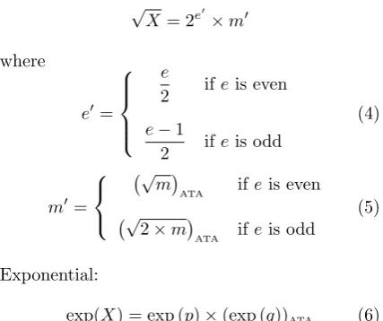
Square Root: √
X = 2e′×m′
where
e′=
e
2 ifeis even
e−1
2 ifeis odd
(4)
m′ =
√
m
ATA ifeis even √
2×m
ATA ifeis odd
(5)
Exponential:
exp(X) = exp (p)×(exp (q))ATA (6)
The reduction tricks for the previously presented function are straightforward. However other ele-mentary functions are more problematic in many senses, e.g., the sine function. The reader should refer to [9] for details about how to do radian reduction over the entire range of floating point number accurately.
There is also a serious problem with straight-forward application of ATA to some elementary functions. Because ATA uses a truncated Taylor polynomial (see next section), there is a problem with the relative error whenX is small as in the first argument values in the sine function. To overcome this problem the input is divided into cases and particular tables are used for each sub-range. See also reference [9] for details.
3. THE ATA METHOD
In the following a short description of Wong and Goto’s ATA method is given (see [8] and [9] for details). Sign and exponent precessing is ignored in any respect. Recall the following definitions:3
• Fraction is the aggregate of the 23-bit of the significant with explicit bit representation in the standard. The number of different frac-tions is 223.
• Mantissa is the normalized number represen-tation of the significant, i.e., it includes the implicit 1 bit and the binary point. Conse-quently, the range of the normalized man-tissa is [1,2) with a resolution of 2−23.
Let X be a fixed point input representing the mantissa of an IEEE Single Precision Floating Point number which is 24 bits in length. How-ever, due to special requirements in handing the exponent, it is sometimes possible to take values outside the [1,2) interval in which the IEEE single precision floating number’s mantissa is obliged to remain. We therefore assumeXto be on different ranges depending on the function as was shown in Table 1.
DivideX into the following chunks,
X =x0+λx1+λ2x2+λ3x3 (7)
3
These denominations may sound inverted but they are compatible with the IEEE standard use for the word frac-tion.
where λ= 2−6, xi <1, i = 1,2,or 3, are 6 bits
in length. On the other hand, depending of the function, we have x0 anywhere in [0,4). Let f
be a function we wish to compute and f(n) be
thenth derivative off. We can write the Taylor polynomial forf as follows
f(X) =
∞
X
n=0
f(n)(x
0+λx1)
n! (λ
2x
2+λ3x3)n (8)
The aim is to approximate f(X) by neglecting terms smaller than λ5. Expanding (8) and
tak-ing the first terms the resulttak-ing equation (9) is the ATA formula. ATA method was proposed by Wong and Goto for the approximation of ele-mentary function for a bounded range [8]. ATA is the acronym for Add-Table lookup-Add, which are the three basic sequential operations required for computing ˜f(X):
1. Add (or subtract) to get the four 13 bit cen-tral differences. x0+λx1+λx2,x0+λx1−
λx2,x0+λx1+λx3,x0+λx1−λx3(the
num-berx0+λx1is obtained by concatenation).
2.1 Read five f values from only one table, or from parallel tables to improve latency.
2.2 Read the last term value, which is a function ofx0 andx2, from a different table4.
3. Add all together the six tables values.
The values stored in the tables are double preci-sion fractional representations in the worst case, i.e., for some tables the length can be shorter than 52-bit.
Wong was able to analytically prove in [7] that, for all the functions and their ranges as given in Table 1, the maximum absolute error is no more than 0.5 ULP.
The author (as in turn Wong and Goto did) wrote a program that makes an exhaustive check of the ATA formula. This is possible because the inputs are 24 bits in length, therefore making it realistic to do so using a computer. The results are shown in Table 2 are identical to those reported in [9] except for the Sine function. The difference may
˜
f(X) = f(x0+λx1) +λ
2 {f(x0+λx1+λx2)−f(x0+λx1−λx2)}+ (9)
λ2
2 {f(x0+λx1+λx3)−f(x0+λx1−λx3)}+λ
4
x2 2
2 f
(2)(x 0)−
x3 2
6 f
(3)(x 0)
4
be due to the use of MatlabR instead of Fortran.
Function Range Error
Reciprocal 1≤X <2 27.3 bit Square Root 1≤X <2 31.6 bit Square Root 2≤X <4 33.3 bit Exponential 0≤X <1 28.3 bit Sine 0≤X < π/2 29.8 bit Natural Logarithm 0.5≤X <1 29.1 bit Natural Logarithm 1≤X <2 29.1 bit Arc Tangent 0≤X <1 29.3 bit
Table 2: Original Maximum Absolute Error
Implementation Details
VHDL language descriptions are not presented due to lack of space. For details see [2]. Ta-bles 3 and 4 present a summary of the relevant characteristics of the design’s components for any elementary function.
Component Characteristic Qt.
Adder 13-bit adder 2
Subtr 13-bit subtracter 2
[image:4.595.88.268.323.495.2]Tree 6-operand adder 1
Table 3: Components
Table Range
T0 and T5 212
T1 and T2 212+ 26−1
T3 and T4 212+ 25−1
Table 4: Table Details
From Table 3 it can be observed that basically only adders are needed. From Table 4 the total tables’ length is just 24,7645.
4. VARYING CHUNK SIZES
Analysis of MAE
Recall that in Table 2 the Error is expressed as a bit position,
Error =−log2MAE (10)
The analysis of MAE from Table 2 and the consid-eration of the reduction tricks demonstrate that the worst case, in the sense of closeness of MARE to 1/2 ULP, corresponds to the Reciprocal. For any other function the accuracy of MAE is fairly larger than is needed. The redundancy is due to the number of bits assigned to the chunks of the mantissa to perform the required accuracy for any function.
5
The ratio 24,764/223
is improper as a performance index.
An Integer Optimization Problem
Looking at equation (9) it can be observed a trade-off between the size of the chunks and the length of the tables demanded. As some others trade-off problems, that can be expressed in terms of an optimization problem. Then, the following integer optimization problem is stated:
Find a mantissa partition6that leads to
the shortest tables for all functions while keeping the MARE s within 0.5 ULP.
In mathematical form, the problem is stated as
Find
min
p TF(p) (11)
subject to
Efi(p)<
ULP
2 ∀i (12)
where p is the unknown mantissa partition, the
objective functionTF(·) is the tables cumulative
length function, the constraints Efi(·) are the
maximum absolute relative error functions, and F = {fi} is the set of all elementary function under consideration.
Furthermore partition p is constrained to four
blocks or chunks as in the original ATA algorithm. In turn,Efi(·) also depends upon particular
nor-malization aspects and upon the maximum abso-lute errors of the ATA formula.
A good approximation to function TF(·) can
be computed straightforward (an example was shown in Table 4).
A definition of partition is needed. For that pur-pose redefine the division ofX into chunks,
X = x0+ 2−p1x1+ (13)
2−(p1+p2)x
2+ 2−(p1+p2+p3)x3
where xi < 1, i = 1,2,or 3 andx0 anywhere in
[0,4). Consequently, equation (9) is easily rein-terpreted.
Any partitions is now characterized by a 3-element vector, pi = [p1 p2 p3]. The original
ATA partition isp0= [ 6 6 6 ]. Proposed Partitions
The analytical solution of the problem is diffi-cult. However. after common sense observations, three candidate partitions (involving shorter ta-bles than the original) are found,
p1= [ 5 6 6 ], p2= [ 6 5 6 ], p3= [ 7 4 6 ]
The proposed partitions are almost identical given thatx0andx1are concatenated in five out
6
of six table addresses (see equation (9)). Actually that fact is a key factor used for the selection of the partitions.
The key criteria for the selection of the partitions are the following:
1. The principal way to reduce table lengths is to reduce the number of bits in the concate-nation between x0 and x1. The proposed
partitions take 11 bit for that concatenation instead of the original 12 bit.
2. The way to control the accuracy of ˆf is vary-ing how many bits are assigned tox0, out of
11 bits.
From the above, it can be observed that just two elements of the partition vector remains as free variables, i.e, the third element is fix in 6. The length of the tables for the proposed parti-tions are shown in Tables 5, 6 and 7. Observe that partition p1 is the most convenient in term
of savings, on the contrary p3 is the less
conve-nient in that respect.
Table Range
T0 and T5 211
T1, T2, T3, and T4 211+ 26−1
Table 5: Table Details forp1
Table Range
T0 211
T1, T2, T3, and T4 211+ 26−1
T5 212
Table 6: Table Details forp2
Table Range
T0 211
T1, T2, T3, and T4 211+ 26−1
T5 213
Table 7: Table Details forp3
The proposed partitions are checked in the next section.
5. SIMULATION AND DISCUSSION
Exhaustive simulation is used again to compute MAE for the new partitions. From the numerous simulations, the extracted results shown in Table 8 are summarize by the following statements:
• Reciprocal: Partitionp3is the only one that
keeps MARE<0.5 ULP.
• Other Functions: Partitionp1 is enough for
the rest of the elementary function consid-ered here.
Function Range p Error
Reciprocal 1≤X <2 p1 23.7 bit
Reciprocal 1≤X <2 p2 24.7 bit
Reciprocal 1≤X <2 p3 25.7 bit
Square Root 1≤X <2 p1 28.2 bit
Square Root 2≤X <4 p1 31.1 bit
Exponential 0≤X <1 p1 26.6 bit
Sine 0≤X < π/2 p1 27.2 bit
Natural Log 1/2≤X <1 p1 25.6 bit
Natural Log 1≤X <2 p1 25.6 bit
Arc Tangent 0≤X <1 p1 25.9 bit
Table 8: Maximum Absolute Error
Formally the optimization goal is reached only when partition p3 is used for all the elementary
functions. Nevertheless, for particular designs, not all the functions addressed here are imple-mented.
As an alternative, different partitions can be used within the same design. In such a case the table length of the correction factor is different for dif-ferent functions. The practical consequence is a complication of the multiplexing. Also different tables can be used for different portions of the range [2].
The reduction in the length of the tables does not necessary have a practical application. Due to technological restrictions, the length of the tables may be an integer power of two. E.g., a table of length 211+ 26−1 must be implemented as one
of length 212.
The worse situation for the utility of the alter-native presented here is the combination of the following four factors:
1. The table lengths are restricted to be an in-teger power of two.
2. A recursive design in which just a single table per function is used.
3. A rigid scheme not allowing the multiplexing of tables of different length.
4. The inclusion of the Reciprocal function.
Under those conditions there is not saving at all when comparing this method with the original ATA.
Suppose the implementation of the Reciprocal function with six parallel tables with lengths re-stricted to an integer power of two. Total table length is 40,960 for partition p0, and 26,624 for
partition p3, i.e., a 35% saving is obtained. For
any other function, under similar conditions, the saving is 50%.
6. CONCLUSIONS
Wong and Goto’s ATA is an arithmetic algorithm for the computation of elementary functions in single precision. ATA is an alternative method to those based not only in pure polynomial approx-imations but also to those based on pure table-lookup. Precisely, the distinction of ATA is the mixing of the two techniques.
This paper presents a modification to the origi-nal ATA method. That change is based on the statement of an optimization problem related to the partition of the mantissa which is central to ATA. The optimization problem is not settled after mathematical concerns but instead after a pragmatic consideration, i.e., the saving of space. That optimization problem is also not solved ana-lytically; instead exhaustive simulations are per-formed. The candidate partitions for the sim-ulations are selected after simple common sense criteria.
For many of the possible implementations, the modification allows a significant saving in space without affecting precision and latency. The sim-ulations show a reduction of table length ranging from approx. 0 to 50% and with minor hardware additions expected.
The VHDL functional descriptions are a by-product of the mixed simulation environment used here. From them is possible to begin the hardware implementation of the components, passing through the register transfer description, all the way to the technological mapping.
REFERENCES
[1] J. Bhasker,A Guide to VHDL Syntax, Pren-tice Hall, 1995.
[2] O. N. Bria and J. O. Giacomantone, “Des-cripciones VHDL para Calcular la Funci´on Rec´ıproca en Presici´on Simple,”Annals VIII Congreso Argentino de Ciencias de la Com-putaci´on, Buenos Aires, Argentina, 2002.
[3] C. Hansen, O. Bringmann. W. Rosenstiel, “A VHDL reusable component model for fixed abstraction level simulation and behav-ioral synthesis,”Virtual Components Design and Reuse, edited by R. Seepold, N. Mart-nez, Kluwer, 2001.
[4] W. Kahan, ”Lecture notes on the status of standard IEEE-754, from the website
http.cs.berkeley.edu/~wkahan/, 1996.
[5] J.-M. Muller, Elementary Functions - Al-gorithms and Implementation, Birkh¨auser, 1997.
[6] B. Parhami, Computer Arithmetic. Algo-rithms and Hardware Designs, Oxford Uni-versity Press, 2000.
[7] W. F. Wong, E. Goto, “Hardware for the Fast Computation of the Elementary Func-tions.” Dr. Eng. Sc. Thesis, University of Tsukuba, Tsukuba, Japan,1995.
[8] W. F. Wong, E. Goto, “Fast hardware-based algorithms for elementary function compu-tations using rectangular multipliers,”IEEE Transactions on Computer, 1994.
[9] W. F. Wong, E. Goto, “Fast evaluation of the elmentary function in single precision,”