Economic Growth – Theory and Numerical Solution Methods

Economic Growth

Alfonso Novales

·

Esther Fernández

·

Jesús Ruiz

Economic Growth

Theory and Numerical Solution Methods

Professor Alfonso Novales Dr. Esther Fernández Dr. Jesús Ruiz

Universidad Complutense

Departamento de Economia Cuantitativa Campus Somosaguas

28223 Pozuelo de Alarcón (Madrid) Spain

anovales@ccee.ucm.es mesferna@ccee.ucm.es jruizand@ccee.ucm.es

ISBN: 978-3-540-68665-1 e-ISBN: 978-3-540-68669-9

Library of Congress Control Number: 2008929527 c

°2009 Springer-Verlag Berlin Heidelberg

This work is subject to copyright. All rights are reserved, whether the whole or part of the material is concerned, specifically the rights of translation, reprinting, reuse of illustrations, recitation, broadcasting, reproduction on microfilm or in any other way, and storage in data banks. Duplication of this publication or parts thereof is permitted only under the provisions of the German Copyright Law of September 9, 1965, in its current version, and permission for use must always be obtained from Springer. Violations are liable to prosecution under the German Copyright Law.

The use of general descriptive names, registered names, trademarks, etc. in this publication does not imply, even in the absence of a specific statement, that such names are exempt from the relevant protective laws and regulations and therefore free for general use.

Cover design: WMX Design GmbH, Heidelberg Printed on acid-free paper

Preface

Integrating Growth Theory and Numerical Solutions

Dynamic, stochastic models with optimizing agents have become a standard tool for policy design and evaluation at central banks and governments around the world. They are also increasingly used as the main reference for forecasting purposes. Such models can incorporate general equilibrium assumptions, as it was the case with Modern Business Cycle Theory, or different types of market frictions, in the form of price rigidity or monopolistic competition, as in the New Keynesian Macroeco-nomics. These models can all be considered as special cases of models of economic growth, and the theoretical and computational methods contained in this book are a first step to get started in this area.

The book combines detailed discussions on theoretical issues on deterministic and stochastic, exogenous and endogenous growth models, together with the com-putational methods needed to produce numerical solutions. A detailed description of the analytical and numerical approach to solving each of the different models covered in the book is provided, and the solution algorithms are implemented in EXCEL and MATLAB files. These files are provided to illustrate theoretical re-sults as well as to simulate the effects of economic policy interventions. Theoretical discussions covered in the book relate to issues such as the inefficiency of the com-petitive equilibrium, the Ricardian doctrine, dynamic Laffer curves, the welfare cost of inflation or the nominal indeterminacy of the price level and local indeterminacy in endogenous growth models, among many others. This integration of theoretical discussions at the analytical level, whenever possible, and numerical solution meth-ods that allow for addressing a variety of additional issues that could not possibly be discussed analytically, is a novel feature of this book.

The Audience

This textbook has been conceived for advanced undergraduate and graduate students in economics, as well as for researchers planning to work with stochastic dynamic growth models of different kinds. As described above, some of the applications

included in the book may be appealing to many young researchers. Analytical dis-cussions are presented in full detail and the reader does not need to have a spe-cific previous background on Growth theory. The accompanying software has been written using the same notation as in the textbook, which allows for an easy under-standing of how each program file addresses a particular theoretical issue. Programs increase in complexity as the book covers more complex models, but the reader can progress easily from the simpler programs in the first chapters to the more com-plex programs in endogenous growth models or programs for analyzing monetary economies. No initial background on programming is assumed.

The book is self contained and it has been designed so that the student advances in the theoretical and the computational issues in parallel. The structure of program files is described in numerical exercise-type of sections, where their output is also interpreted. These sections should be considered an essential part of the learning process, since the provided program files can be easily changed following our indi-cations so that the reader can formulate and analyze his/her own questions.

Main Ideas

Exogenous and endogenous growth models are thoroughly reviewed throughout the book, and special attention is paid to the use of these models for fiscal and monetary policy analysis. The structure of each model is first presented, and the equilibrium conditions are analytically characterized. Equilibrium conditions are interpreted in detail, with special emphasis on the role of the transversality condition in guaran-teeing the stability of the implied solution. Stability is a major issue throughout the book, and a central ingredient in the construction of the solution algorithms for the different models.

The illustrations used in the ‘Numerical Exercise’-type sections throughout the book discuss a variety of characteristics of the numerical solution to each specific model, including the evaluation of some policy experiments. Most issues considered in these sections, like the details of the numerical simulation of models with techno-logical diffusion or Schumpeterian models under uncertainty are presented for the first time in a textbook, having appeared so far only in research papers.

Brief Description of Contents

The use of rational expectations growth models for policy analysis is discussed in the Introductory chapter, where the need to produce numerical solutions is ex-plained. Chapter 2 presents the neoclassical Solow–Swan growth model with con-stant savings, in continuous and discrete time formulations. Chapter 3 is devoted to the optimal growth model in continuous time. The existence of an optimal steady state is shown and stability conditions are characterized. The relationship between the resource allocations emerging from the benevolent planner’s problem and from the competitive equilibrium mechanism is shown. The role of the government is ex-plained, fiscal policy is introduced and the competitive equilibrium in an economy with taxes is characterized. Finally, the Ricardian doctrine is analyzed. Chapter 4 addresses the same issues in discrete time formulation, allowing for numerical solu-tions to be introduced and used for policy evaluation. Deterministic and stochastic versions of the model are successively considered.

Chapter 5 is devoted to solution methods and their application to solving the op-timal growth model of an economy subject to distortionary and non-distortionary taxes. The chapter covers some linear solution methods, implemented on linear and log-linear approximations: the linear-quadratic approximation, the undetermined coefficients method, the state-space approach, the method based on eigenvalue-eigenvector decompositions of the approximation to the model, and also some non-linear methods, like the parameterized expectations model and a class of projection methods. Special emphasis is placed on the conditions needed to guarantee stability of the implied solutions.

possibilities for the design of a mix of fiscal and monetary policy in economies with and without distorting taxation are discussed. Conditions for the non-neutrality of monetary policy under endogenous labour supply are examined. The chapter closes with a description of the Ramsey problem that describes the choice of optimal mon-etary policy. Chapter 9 characterizes the transitional dynamics in deterministic and stochastic monetary economies and presents numerical solution methods for terministic and stochastic monetary economies. Specific details are provided de-pending on whether the monetary authority uses nominal interest rates or the rate of growth of money supply as a control variable for monetary policy implementa-tion. Special attention is paid to the possibility of nominal indeterminacy arising as a consequence of the specific design followed for monetary policy. The chapter closes with a presentation of Keynesian monetary models, which are increasingly used for actual policy making. After characterizing equilibrium conditions, a numerical so-lution approach is discussed in detail.

A more detailed synopsis of the book is provided in Sect. 1.5.

Software

As explained above, MATLAB and EXCEL files are provided to analyze a variety of theoretical issues. EXCEL files are used to compute a single realization of the solution to a given model. That is enough in deterministic economies. There are also MATLAB programs that perform the same analysis. In stochastic economies, however, characterizing the probability distribution of a given statistic through a large number of realizations becomes impossible in a spreadsheet, and it is done in MATLAB programs. All MATLAB and EXCEL files are downloadable from our Web page: www.ucm.es/info/ecocuan/anc/Growth/growthbook.htm

Antecedents and Acknowledgments

Over the years, we have benefited from working through textbooks on Economic Growth and Dynamic General Equilibrium Economies [Barro and Sala-i-Martin (2003), Aggion and Howitt (1999), Stokey and Lucas (1989), Blanchard and Fisher (1998), Lucas (1987), Sargent (1987), Ljunquist and Sargent (2004), Hansen y Sargent (2005), Cooley (1995), Turnovsky (2000), Walsh (1998)], who obviously should not be held accountable for any misconception that might arise in this volume.

(2002), McCandless (2008)] provide additional reading, in some cases with alter-native approaches to model solution.

The idea that any dynamic model has time series implications that can be put to test with actual data has traditionally been a central premise in the graduate pro-grams in Economics at University of Minnesota, and has clearly influenced the conception of this book. Specially important to us were the teachings of Stephen Turnovsky, Tom Sargent and Christopher Sims. In that context, it was easy to under-stand that advances in Economics should come from iterating between theoretical models and actual data and from there, the need to obtain statistical implications from any model economy.

Previous versions of parts of this book have been used in advanced undergrad-uate and gradundergrad-uate courses in Economics and Quantitative Finance at Universidad Complutense (Madrid, Spain), City University of Yokohama (Yokohama, Japan) and Keio University (Tokyo, Japan). We appreciate the patience of students working out details of previous drafts.We thank Yoshikiyo Sakai and Yatsuo Maeda for the opportunity to discuss this material while still in process. We are greatly indebted with our friends and colleagues Emilio Dom´ınguez, Javier P´erez and Gustavo Mar-rero for many useful and illuminating discussions. Finally, our deepest gratitude to our families for their understanding through the long and demanding process of producing this book.

1 Introduction. . . 1

1.1 A Few Time Series Concepts . . . 2

1.1.1 Some Simple Stochastic Processes . . . 3

1.1.2 Stationarity, Mean Reversion, Impulse Responses . . . 6

1.1.3 Numerical Exercise: Simulating Simple Stochastic Processes . . . 9

1.2 Structural Macroeconomic Models . . . 12

1.2.1 Static Structural Models . . . 12

1.2.2 Dynamic Structural Models . . . 16

1.2.3 Stochastic, Dynamic Structural Models . . . 21

1.2.4 Stochastic Simulation . . . 23

1.2.5 Numerical Exercise – Simulating Dynamic, Structural Macroeconomic Models . . . 24

1.3 Why are Economic Growth Models Interesting? . . . 27

1.3.1 Microeconomic Foundations of Macroeconomics . . . 27

1.3.2 Lucas’ Critique on Economic Policy Evaluation . . . 33

1.3.3 A Brief Overview of Developments on Growth Theory . . . 35

1.3.4 The Use of Growth Models for Actual Policy Making . . . 39

1.4 Numerical Solution Methods . . . 40

1.4.1 Why do we Need to Compute Numerical Solutions to Growth Models? . . . 40

1.4.2 Stability . . . 42

1.4.3 Indeterminacy . . . 43

1.4.4 The Type of Questions We Ask and the Conclusions We Reach . . . 44

1.5 Synopsis of the Book . . . 48

2 The Neoclassical Growth Model Under a Constant Savings Rate. . . 53

2.1 Introduction . . . 53

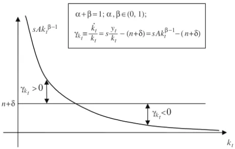
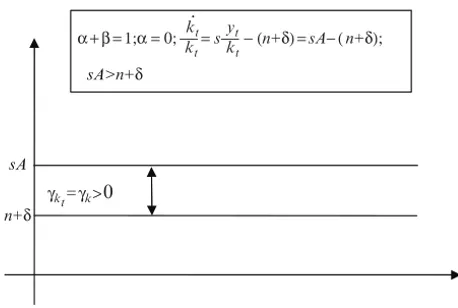
2.2 Returns to Scale and Sustained Growth . . . 54

2.3 The Neoclassical Growth Model of Solow and Swan . . . 59

2.3.1 Description of the Model . . . 60

2.3.2 The Dynamics of the Economy . . . 61

2.3.3 Steady-State . . . 64

2.3.4 The Transition Towards Steady-State . . . 68

2.3.5 The Duration of the Transition to Steady-State . . . 69

2.3.6 The Growth Rate of Output and Consumption . . . 69

2.3.7 Convergence in the Neoclassical Model . . . 71

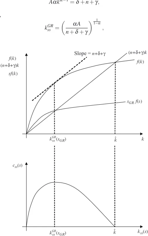
2.3.8 A Special Steady-State: The Golden Rule of Capital Accumulation . . . 73

2.4 Solving the Continuous-Time Solow–Swan Model . . . 76

2.4.1 Solution to the Exact Model . . . 76

2.4.2 The Linear Approximation to the Solow–Swan Model . . . 77

2.4.3 Changes in Structural Parameters . . . 79

2.4.4 Dynamic Inefficiency . . . 82

2.5 The Deterministic, Discrete-Time Solow Swan Model . . . 85

2.5.1 The Exact Solution . . . 85

2.5.2 Approximate Solutions to the Discrete-Time Model . . . 87

2.5.3 Numerical Exercise – Solving the Deterministic Solow–Swan Model . . . 89

2.5.4 Numerical Exercise – A Permanent Change in the Savings Rate . . . 91

2.5.5 Numerical Exercise – Dynamic Inefficiency . . . 93

2.6 The Stochastic, Discrete Time Version of the Solow–Swan Model . . 95

2.6.1 Numerical Exercise – Solving the Stochastic Solow–Swan Model . . . 96

2.7 Exercises . . . 98

3 Optimal Growth. Continuous Time Analysis . . . 101

3.1 The Continuous-Time Version of the Cass–Koopmans Model . . . 101

3.1.1 Optimality Conditions for the Cass–Koopmans Model . . . 103

3.1.2 The Instantaneous Elasticity of Substitution of Consumption (IES) . . . 104

3.1.3 Risk Aversion and the Intertemporal Substitution of Consumption . . . 106

3.1.4 Keynes–Ramsey Condition . . . 107

3.1.5 The Optimal Steady-State . . . 108

3.1.6 Numerical Exercise: The Sensitivity of Steady-State Levels to Changes in Structural Parameters . . . 110

3.1.7 Existence, Uniqueness and Stability of Long-Run Equilibrium – A Graphical Discussion . . . 112

3.1.8 Suboptimality of the Golden Rule . . . 114

3.2 Stability and Convergence . . . 115

3.2.2 Numerical Exercise – Characterizing the Transition

after a Change in a Structural Parameter . . . 120

3.3 Interpreting the Central Planners’s Model as a Competitive Equilibrium Economy . . . 126

3.3.1 The Efficiency of Competitive Equilibrium . . . 129

3.4 A Competitive Equilibrium with Government . . . 131

3.4.1 The Structure of the Economy . . . 131

3.4.2 Feasible Stationary Public Expenditure and Financing Policies . . . 135

3.4.3 Competitive Equilibrium . . . 135

3.4.4 Global Constraint of Resources . . . 136

3.4.5 The Representative Agent Problem . . . 136

3.5 On the Efficiency of Equilibrium with Government . . . 138

3.5.1 On the Efficiency of Equilibrium Under Lump-Sum Taxes and Debt . . . 138

3.5.2 The Inefficiency of the Competitive Equilibrium Allocation Under Distortionary Taxes . . . 140

3.6 The Ricardian Doctrine . . . 146

3.6.1 The Ricardian Doctrine Under Non-Distorting Taxes . . . 146

3.6.2 Failure of the Ricardian Doctrine Under Distorting Taxes . . . 147

3.7 Appendix . . . 149

3.7.1 Appendix 1 – Log-linear Approximation to the Continuous Time Version of Cass–Koopmans Model . . . 149

3.7.2 Appendix 2 – An Alternative Presentation of the Equivalence Between the Planner’s and the Competitive Equilibrium Mechanisms in an Economy Without Government . . . 150

3.8 Exercises . . . 153

4 Optimal Growth. Discrete Time Analysis . . . 155

4.1 Discrete-Time, Deterministic Cass–Koopmans Model . . . 155

4.1.1 The Global Constraint of Resources . . . 155

4.1.2 Discrete-Time Formulation of the Planner’s Problem . . . 157

4.1.3 The Optimal Steady-State . . . 158

4.1.4 The Dynamics of the Model: The Phase Diagram . . . 159

4.1.5 Transversality Condition in Discrete Time . . . 161

4.1.6 Competitive Equilibrium with Government . . . 162

4.2 Fiscal Policy in the Cass–Koopmans Model . . . 167

4.2.1 The Deterministic Case . . . 167

4.2.2 Numerical Exercise – Solving the Deterministic Competitive Equilibrium with Taxes . . . 176

4.2.3 Numerical Exercise – Fiscal Policy Evaluation . . . 179

4.3 Appendices . . . 185

4.3.2 The Intertemporal Government Budget Constraint . . . 187

4.4 Appendix 2: The Ricardian Proposition Under Non-Distortionary Taxes in Discrete Time . . . 190

4.5 Exercises . . . 191

5 Numerical Solution Methods . . . 195

5.1 Numerical Solutions and Simulation Analysis . . . 195

5.2 Analytical Solutions to Simple Growth Models . . . 197

5.2.1 A Model with Full Depreciation . . . 197

5.2.2 A Model with Leisure in the Utility Function . . . 200

5.2.3 Numerical Solutions of the Growth Model Under Full Depreciation . . . 202

5.3 Solving a Simple, Stochastic Version of the Planner’s Problem . . . 203

5.3.1 Solving the Linear-Quadratic Approximation to the Planner’s Problem . . . 204

5.3.2 The Log-Linear Approximation to the Model . . . 210

5.3.3 The Blanchard–Kahn Solution Method for the Stochastic Planner’s Problem. Log-Linear Approximation . . . 212

5.3.4 Uhlig’s Undetermined Coefficients Approach. Log-Linear Approximation . . . 215

5.3.5 Sims’ Eigenvalue-Eigenvector Decomposition Method Using a Linear Approximation to the Model . . . 217

5.4 Solving the Stochastic Representative Agent’s Problem with Taxes . . . 225

5.4.1 The Log-Linear Approximation . . . 227

5.4.2 Numerical Exercise: Solving the Stochastic Representative Agent’s Model with Taxes Through Blanchard and Kahn’s Approach. Log-Linear Approximation . . . 228

5.4.3 Numerical Exercise: Computing Impulse Responses to a Technology Shock. Log-Linear Approximation . . . 232

5.4.4 Numerical Exercise: Solving the Stochastic Representative Agent’s Model with Taxes Through the Eigenvector and Eigenvalue Decomposition Approach. Linear Approximation . . . 234

5.5 Nonlinear Numerical Solution Methods . . . 238

5.5.1 Parameterized Expectations . . . 238

5.5.2 Projection Methods . . . 241

5.6 Appendix – Solving the Planner’s Model Under Full Depreciation . . 251

5.7 Exercises . . . 253

6 Endogenous Growth Models. . . 257

6.1 TheAKModel . . . 257

6.1.1 Balanced Growth Path . . . 259

6.1.2 Transitional Dynamics . . . 259

7.3.4 Numerical Exercise: Solving the Model with Varieties

of Intermediate Goods, and the Diffusion Growth Model . . . 332

7.4 Schumpeterian Growth . . . 333

7.4.1 The Economy . . . 334

7.4.2 Computing Equilibrium Trajectories . . . 338

7.4.3 Deterministic Steady-State . . . 341

7.5 Endogenous Growth with Accumulation of Human Capital . . . 342

7.5.1 The Economy . . . 343

7.5.2 The Competitive Equilibrium . . . 347

7.5.3 Analyzing the Deterministic Steady-State . . . 349

7.5.4 Numerical Exercise: Steady-State Effects of Fiscal Policy . . 352

7.5.5 Computing Equilibrium Trajectories in a Stochastic Setup Under the Assumption of Rational Expectations . . . 353

7.5.6 Indeterminacy of Equilibria . . . 363

7.5.7 Numerical Exercise: The Correlation Between Productivity and Hours Worked in the Human Capital Accumulation Model . . . 374

7.6 Exercises . . . 376

8 Growth in Monetary Economies: Steady-State Analysis of Monetary Policy. . . 377

8.1 Introduction . . . 377

8.2 Optimal Growth in a Monetary Economy: The Sidrauski Model . . . . 378

8.2.1 The Representative Agent’s Problem . . . 380

8.2.2 Steady-State in the Monetary Growth Economy . . . 384

8.2.3 Golden Rule . . . 387

8.3 Steady-State Policy Analysis . . . 388

8.3.1 Optimal Steady-State Rate of Inflation . . . 389

8.3.2 The Welfare Cost of Inflation . . . 392

8.4 Two Modelling Issues: Nominal Bonds and the Timing of Real Balances . . . 394

8.4.1 Nominal Bonds: The Relationship Between Real and Nominal Interest Rates . . . 395

8.4.2 Real Balances in the Utility Function: At the Beginning or at the End of the Period? . . . 397

8.4.3 Numerical Exercise: Optimal Rate of Inflation Under Alternative Assumptions on Preferences . . . 400

8.5 Monetary Policy Analysis Under Consumption and Income Taxes . . 401

8.5.1 Steady-State . . . 403

8.5.2 Numerical Exercise: Computation of Steady-State Levels Under Alternative Policy Choices . . . 405

8.6 Monetary Policy Under Endogenous Labor Supply . . . 406

8.6.1 The Neutrality of Monetary Policy Under Endogenous Labor Supply . . . 406

8.7 Optimal Monetary Policy Under Distortionary Taxation

and Endogenous Labor . . . 413

8.7.1 The Model . . . 414

8.7.2 Implementability Condition . . . 417

8.7.3 The Ramsey Problem . . . 418

8.8 Exercises . . . 419

9 Transitional Dynamics in Monetary Economies: Numerical Solutions. . . 423

9.1 Introduction . . . 423

9.2 Stability of Public Debt . . . 424

9.3 Alternative Strategies for Monetary Policy: Control of Nominal Rates vs. Money Growth Control . . . 426

9.4 Deterministic Monetary Model with the Monetary Authority Choosing Money Growth . . . 427

9.4.1 Steady-State . . . 429

9.4.2 Solution Through a Log-Linear Approximation . . . 430

9.4.3 Complex Eigenvalues . . . 433

9.5 Deterministic Monetary Model with the Monetary Authority Choosing Nominal Interest Rates . . . 437

9.6 Transitional Effects of Policy Interventions . . . 441

9.6.1 Solving the Model with Nominal Interest Rates as Control Variable, Using a Linear Approximation . . . 442

9.6.2 Numerical Exercise: Changes in Nominal Interest Rates . . . . 444

9.6.3 Solving the Model with Money Growth as Control Variable, Using a Linear Approximation . . . 445

9.6.4 Numerical Exercise: Gradual vs. Drastic Changes in Money Growth . . . 448

9.7 The Stochastic Version of the Monetary Model . . . 450

9.7.1 The Monetary Authority Chooses Nominal Interest Rates . . 452

9.7.2 The Monetary Authority Chooses Money Supply Growth . . . 463

9.8 A New Keynesian Monetary Model . . . 469

9.8.1 A Model Without Capital Accumulation: Ireland’s (2004) . . 470

9.8.2 A New Keynesian Monetary Model with Capital Accumulation . . . 477

9.9 Appendix: In a Log-Linear Approximation,Etπˆt+1=ıˆt−rˆt. . . 491

9.10 Exercises . . . 492

10 Mathematical Appendix . . . 495

10.1 The Deterministic Control Problem in Continuous Time . . . 495

10.1.1 Transversality Condition . . . 496

10.1.2 The Discounted Problem . . . 496

10.1.3 Calculus of Variations . . . 498

10.2 The Deterministic Control Problem in Discrete Time . . . 499

10.3.1 1. First Order Differential Equations with Constant

Coefficients . . . 501

10.3.2 2. First Order Differential Equations with Variable Coefficients . . . 504

10.4 Matrix Algebra . . . 506

10.4.1 The 2×2 Case . . . 508

10.4.2 Systems with a Saddle Path Property . . . 510

10.4.3 Imposing Stability Conditions Over Time . . . 510

10.5 Some Notes on Complex Numbers . . . 513

10.6 Solving a Dynamic Two-Equation System with Complex Roots . . . . 514

References. . . 517

Introduction

This is a book on Growth Theory and on the numerical methods needed to fully characterize the properties of most Growth models. In this introductory chapter, we describe the main characteristics of different families of Growth models and their relevance for policy analysis, which is moving leading economic and financial insti-tutions throughout the world to increasingly rely on their use for forecasting as well as for policy evaluation. In particular, we emphasize how the richer structure pro-vided to Growth models by their Microeconomic foundations allows us to address a much broader set of policy issues than in more traditional structural dynamic els. The book gradually builds on by increasing the degree of generality of the mod-els being considered, as explained below. We cover: (a) neoclassical growth under a constant savings rate, (b) optimal growth, (c) numerical solution methods, (d) en-dogenous growth, and (e) monetary growth. Theoretical discussions on each model are presented, with special attention to characterizing the properties of equilibrium solutions and their use for fiscal policy considerations, while a specific chapter deals with monetary policy issues. Algorithms to solve all models considered are pre-sented, together with EXCEL spreadsheets and MATLAB programs that implement them. Results obtained by these programs are commented in “Numerical exercise ”-type sections, where some indications are provided on possible modifications of the enclosed programs. The book has been written with the intention that it may be accessible to students without an initial background on Growth Theory or mathe-matical software. Maintaining the same notation used in the analytical presentations in the book should allow the reader to follow easily the structure of the programs and quickly learn how to adapt them to alternative specifications or theoretical as-sumptions.

Growth models incorporate very specific assumptions on the structure of pref-erences, technology, the sources of randomness, and the policy rules followed by the economic authority, and characterize the relationship implied by such a struc-ture between the decisions made by the different agents at each point in time and the information they have available when making their decisions. Under uncertainty, agents’ perceptions on the future are an explicit determinant of their actions. Growth models do not make ad-hoc assumptions on the way how expectations influence

A. Novales et al.,Economic Growth: Theory and Numerical Solution Methods, 1 c

agents’ decisions. Rather, the solution to the optimization problems posed for each agent leads to decision rules for the different agents that incorporate expectations of functions of future variables in a very specific manner. If expectations are assumed to be rational, expectations in the model become endogenous variables, they are fully consistent with the structure of the model, and incorporate agents’ perceptions of possible future changes in policy. Doing that, these models are safe from a strong criticism made on a traditional approach to economic policy evaluation by Nobel laureate R.E. Lucas that has been very influential in the last decades. This is the reason why, as we describe below, these models are increasingly being used in the research departments of Central Banks and main international economic institutions to forecast as well as to evaluate the consequences of alternative policy choices.

The counterpart comes from the fact that the type of stochastic control problems that are integrated into a Growth model lack an analytical solution, so they need to be solved following a numerical approach, accompanied by Monte Carlo simula-tion in the case of stochastic Growth models. The numerical solusimula-tion to the model then comes in the form of artificial time series that can be analyzed using stan-dard statistical and econometric tools, and the results compared to those obtained in corresponding time series data from actual economies. These are the main is-sues introduced in this chapter, which are later gradually developed throughout the book. Section 1.1 reviews some statistical concepts using simple time series models, Sect. 1.2 considers some simple dynamic macroeconomic models in which we in-troduce additional concepts, as well as the fundamentals of the simulation methods that will be used through the book. Section 1.3 introduces the main characteristics of Growth models, in comparison with more traditional dynamic macroeconomic models. This section motivates the convenience to work with Growth models and describes their different types, paying attention to the way they deal with the criti-cism to more traditional policy evaluation. Section 1.4 explains the need to obtain numerical solutions to Growth models, their potential use, and how this approach has led to changing the type of policy questions we ask and the type of answers we get. This introductory chapter ends up with a synopsis of the book, where a reference is made to the treatment of the issues mentioned along this Introduction.

1.1 A Few Time Series Concepts

process, which would likely be assumed to be zero in the case of asset returns. If returns are logarithmic, i.e., the first difference of logged market prices, then prices themselves would follow a random walk structure. These properties cannot be ar-gued separately from each other, since they are just two different forms of making the same statement on stock market prices. We may also say at some point that the economy is likely to repeat next year its growth performance from the previous year, which incorporates the belief that annual GNP growth follows a random walk, its best one-step ahead prediction being the last observed value. A high persistence in real wages or in inflation could be consistent with first order autoregressive mod-els with an autoregressive parameter close to 1. We briefly review in this section some concepts regarding basic stochastic processes, of the type that are often used to represent the behavior of economic variables.

1.1.1 Some Simple Stochastic Processes

A stochastic process is a sequence of random variables indexed by time. Each of the random variables in a stochastic process, corresponding to a given time indext, has its own probability distribution. These distributions can be different, and any two of the random variables in a stochastic process may either exhibit dependence of some type or be independent from each other.

Awhite noiseprocess is,

yt=εt, t=1,2,3, ...

whereεt,t=1,2, ...is a sequence of independent, identically distributed zero-mean

random variables, known as theinnovationto the process. A white noise is some-times defined by adding the assumption thatεthas a Normal distribution. The

math-ematical expectation of a white noise is zero, and its variance is constant:Var(yt) =

σ2

ε.More generally, we could consider awhite noise with constant, by incorporating a constant term in the process,

yt=a+εt, t=1,2,3, ...

with mathematical expectationE(yt) =a, and variance:Var(yt) =σ2_ε.

The future value of a white noise with drift obeys,

yt+s=a+εt+s,

so that, if we try to forecast any future value of a white noise on the basis of the information available1at timet, we would have:

Etyt+s=a+Etεt+s=a,

1_{That amounts to constructing the forecast by application of the conditional expectation operator to}

because of the properties of theεt-process. That is, the prediction of a future value

of a white noise is given by the mean of the process. In that sense, a white noise process isunpredictable. The prediction of such process is given by the mean of the process, with no effect from previously observed values. Because of that, the history of a white noise process is irrelevant to forecast its future values. No matter how many data points we have, we will not use them to forecast a white noise.

Arandom walk with driftis a process,

yt=a+yt−1+εt, t=1,2,3, ... (1.1)

so that its first differences are white noise. Ifyt=ln(Pt)is the log of some market

price, then its return rt =ln(Pt)−ln(Pt−1),will be a white noise, as we already

mentioned. A random walk does not have a well defined mean or variance. In the case of arandom walk without drift, we have,

yt+s=yt+s−1+εt+s, s≥1

so that we have the sequence of forecasts:

Etyt+1=Etyt+Etεt+1=yt,

Etyt+2=Etyt+1+Etεt+2=Etyt+1=yt,

and the same for all future variables. In this case, the history of a random walk process is relevant to forecast its future values, but only through the last observation. All data points other than the last one are ignored when forecasting a random walk process.

First order autoregressive processes,AR(1), are of the form,

yt=ρyt−1+εt,|ρ|<1,

and can be represented by,

yt=

∞

∑

s=0 ρs_ε

t−s,

the right hand side having a finite variance under the assumption thatVar(εt) =σ2_ε

only if|ρ|<1.In that case, we would have:

E(yt) =0; Var(yt) = σ

2 ε 1−ρ2.

Predictions from a first order autoregression can be obtained by,

Etyt+1=ρEtyt+Etεt+1=ρyt,

Etyt+2=Et(ρyt+1) +Etεt+2=ρ2Etyt+1=ρ2yt,

and, in general,

which is the reason to impose the constraint|ρ|<1.The parameterρis sometimes known as thepersistenceof the process. As the previous expression shows, an in-crease or dein-crease inyt will show up in any futureyt+s,although the influence of

thatyt-value will gradually disappear over time, according to the value ofρ.A value

ofρclose to 1 will therefore introduce high persistence in the process, the opposite being true forρclose to zero.

The covariance between the values of the first order autoregressive process at two points in time is:

Cov(yt,yt+s) =ρsVar(yt),s≷0,

so that the linear correlation is:

Corr(yt,yt+s) =

Cov(yt,yt+s)

Var(yt)

=ρs,

which dies away at a rate ofρ.In an autoregressive process with a value ofρclose to 1, the correlation ofytwith past values will be sizeable for a number of periods.

A first order autoregressive process with constant has the representation,

yt=a+ρyt−1+εt,|ρ|<1.

Let us assume by now that the mathematical expectation exists and is finite. Un-der that assumption,Eyt=Eyt−1, and we have:

Eyt=a+E(ρyt−1) +Eεt=a+ρEyt,

so that:Eyt =_1−ρa .To find out the variance of the process, we can iterate on its

representation:

yt =a+ρyt−1+εt=a+ρ(a+ρyt−2+εt−1) +εt

=a(1+ρ+ρ2+...+ρs−1) +ρsyt−s +ρs−1εt−s+1+...+ρ2εt−2+ρεt−1+εt

,

and if we proceed indefinitely, we get

yt=a(1+ρ+ρ2+...) +

...+ρ2εt−2+ρεt−1+εt

,

since lim

s→∞ρ

s_y

t−s=0.2Then, taking the variance of this expression:

Var(yt) =Var

...+ρ2εt−2+ρεt−1+εt

=

∞

∑

s=0 ρ2s_σ2

ε= σ 2 ε 1−ρ2,

so that the variance of theyt-process increases with the variance of the innovation,

σ2

ε, but it is also higher the closer is ρ to 1. As ρ approaches 1, the first order

2_{This is the limit of a random variable, and an appropriate limit concept must be used. It suffices}

autoregression becomes a random walk, for which this expression would give an infinite variance. This is because if we repeat for the random walk the same argu-ment we have made here, we get,

yt =a+yt−1+εt=a+ (a+yt−2+εt−1) +εt

=as+yt−s+ (εt−s+1+...+εt−2+εt−1+εt),

so that the past termyt−sdoes not die away no matter how far we move back into the

past, and the variance of the sum in brackets increases without bound as we move backwards in time. The random walk process has an infinite variance. Sometimes, it can be assumed that there is a known initial conditiony0.The random walk process can then be represented:

yt =a+yt−1+εt=a+ (a+yt−2+εt−1) +εt

=...=at+y0+ (ε1+...+εt−2+εt−1+εt),

withE(yt) =taandVar(yt) =tσ2_ε. Hence, both moments change over time, the

variance increasing without any bound. However, if we compare in a same graph time series realizations of a random walk together with some stationary autoregres-sive processes, it will be hard to tell which is the process with an infinite variance.

A future value of the first order autoregression can be represented:

yt+s=a+ρyt+s−1+εt+s,|ρ|<1, s≥1,

which can be iterated to,

yt+s=a(1+ρ+ρ2+...+ρs−1) +ρsyt+

ρs−1_ε

t+1+ρs−2εt+2+...+εt+s

,

so that its forecast is given by,

yt+s=a

1−ρs 1−ρ +ρ

s_y t.

So, as the forecast horizon goes to infinity, the forecast converges to,

limEtyt+s=

a

1−ρ,

the mean of the process.

1.1.2 Stationarity, Mean Reversion, Impulse Responses

A stochastic process is stationary when the distribution ofk-tuples(yt1,yt2, . . . ,ytk)

is the same with independence of the value ofkand of the time periodst1,t2, . . . ,tk

a future value converges to its mean as the forecast horizon goes to infinity. This is obviously fulfilled in the case of a white noise process. Another characteristic is that any time realization crosses the sample mean often, while a nonstationary process would spend arbitrarily large periods of time at either side of its sample mean. As we have seen above for the first order autoregression, the simple autocorrelation function of a stationary process, made up by the sequence of correlations between any two values of the process, will go to zero relatively quickly, dieing away very slowly for processes close to nonstationarity.

When they are not subject to an stochastic innovation,3 stationary autoregres-sive processes converge smoothly and relatively quickly to their mathematical ex-pectation. Theyt-process will converge to _1−ρa either from above or from below,

depending on whether the initial value,y0,is above or below _1−ρa .The speed of convergence is given by the autoregessive coefficient. When the process is subject to a nontrivial innovation, the convergence in the mean of the process will not be easily observed. This is the case because the process experiences a shock through the innovation process every period, which would start a new convergence that would overlap the previous one, and so on. Under normal circumstances we will just see a time realization exhibiting fluctuations around the mathematical expectation of the process, unless the process experiences a huge innovation, or the starting condition

y0is far enough from_1−ρa ,in units of its standard deviation,

σ2

ε

1−ρ2.

The property of converging to the mean after any stochastic shock is calledmean reversion, and is characteristic of stationary processes. In stationary processes, any shock tends to be corrected over time. This cannot be appreciated because shocks to

yt are just the values of the innovation process, which take place every period. So,

the process of mean reversion following a shock gets disturbed by the next shock, and so on. But the stationary process will always react to shocks as trying to return to its mean. Alternatively, a non stationary process will tend to depart from its mean following any shock. As a consequence, the successive values of the innovation processεt will takeyt every time farther away from its mean.

An alternative way of expressing this property is through the effects of purely transitory shocks or innovations. A stationary process has transitory responses to purely transitory innovations. On the contrary, a nonstationary process may have permanent responses to purely transitory shocks. So, if a stationary variable experiences a one-period shock, its effects may be felt longer than that, but will disappear after a few periods. The effects of such a one-period shock on a non-stationary process will be permanent. A white noise is just an innovation process. The value taken by the white noise process is the same as that taken by its inno-vation. Hence, the effects of any innovation last as long as the innovation itself, reflecting the stationary of this process. The situation with a random walk is quite different. A random walk takes a value equal to the one taken the previous period, plus the innovation. Hence, any value of the innovation process gets accumulated in successive values of the random walk. The effects of any shock last forever,

reflect-3_{That is, if the innovationε}

ing the nonstationary nature of this process. In a stationary first order autoregression, any value of the innovationεtgets incorporated intoytthat same period. It will also

have an effect of size ρεt onyt+1. This is becauseyt+1=ρyt+εt+1so, even if εt+1=0,the effect ofεt would still be felt onyt+1through the effect it previously had onyt.

This argument suggests how to construct what we know as animpulse response function. In the case of a single variables, as with the stochastic processes we con-sider in this section, that response is obtained by setting the innovation to zero every period except one, in which the impulse is produced. At that time, the innovation takes a unit value.4The impulse response function will be the difference between the values taken by the process after the impulse in its innovation, and those that would have prevailed without the impulse. The response of a white noise to an im-pulse in its own innovation is a single unit peak at the time of the imim-pulse, since the white noise is every period equal to its innovation, which is zero except at that time period. In the case of a general random walk, a zero innovation would lead to a random walk growing constantly at a rate defined by the driftafrom a given initial conditiony0. If at timet∗the innovation takes a unit value, the random walk will increase by that amount at timet∗,but also at any future time. So the impulse response is in this case astep function, that takes the value 1 att∗and at any time after that. Consider now a stationary first order autoregression. A unit innovation at timet∗will have a unit response at that time period, and a response of sizeρseach periodt+s,gradually decreasing to zero.

Another important characteristic of economic time series is the possibility that they exhibit cyclical fluctuations. In fact, first order autoregressive processes may display a shape similar to that of many economic time series, although to produce regular cycles we need a second order autoregressive processes,

yt=ρ1yt−1+ρ2yt−2+εt,

withεt being an innovation, a sequence of independent and identically distributed

over time. Using the lag operator:Bs_y

t=yt−sin the representation of the process:

yt−ρ1yt−1−ρ2yt−2=

1−ρ₁B−ρ₂B2yt=εt.

The dynamics of this process is characterized by the roots of its characteristic equation,

1−ρ₁B−ρ₂B2= (1−λ+B) (1−λ−B) =0,

which are given by:

λ+,λ−= −ρ1±

ρ2

1+4ρ2

2ρ₂ .

4_{When working with several variables, responses can be obtained for impulses in more than one}

Stationary second order autoregressions have the two roots of the characteristic equation smaller than 1. A root greater than one in absolute size will produce an explosive behavior. A root equal to one also signals nonstationarity, although the sample realization will not be explosive. It will display extremely persistent fluctu-ations, very rarely crossing its mean, as it was the case with a random walk. This is very clear in the similar representation of a random walk:(1−B)yt=εt.

Since the characteristic equation is now of second degree, it might have as roots two conjugate complex numbers. When that is the case, the autoregressive process displays cyclical fluctuations. The response ofytto an innovationεtwill also display

cyclical fluctuations, as we will see in dynamic macroeconomic models below.

1.1.3 Numerical Exercise: Simulating Simple Stochastic Processes

TheSimple simulation.xlsEXCEL book presents simulations of some of these sim-ple stochastic processes. Column A in the Simulations spreadsheet contains a time index. Column B contains a sample realization of random numbers extracted from a N(0,1) distribution. This has been obtained from EXCEL using the sequence of keys:Tools/Data Analysis/Random Number Generatorand selecting as options in the menunumber of variables=1,observations =200, aNormaldistribution with expectation 0 and variance 1, and selecting the appropriate output range in the spreadsheet.

A well constructed random number generator produces independent realizations of the chosen distribution. We should therefore have in column B 200 independent data points from a N(0,1), which can either be interpreted as a sample of size 200 from a N(0,1) population, or as a single time series realization from a white noise where the innovation follows a N(0,1) probability distribution. The latter is the inter-pretation we will follow. At the end of the column, we compute the sample mean and standard deviation, with values of 0.07 and 1.04, respectively. These are estimates of the 0 mathematical expectation and unit standard deviation with this sample. Be-low that, we present the standard deviation of the first and the last 100 observations, of 1.05 and 1.03. Estimates of the variance obtained with the full sample or with the two subsamples seem reasonable. A different sample would lead to different numerical estimates.

to try to interpret such statistics. In particular, in this case, by drawing different realizations for the white noise in column B, the reader can easily check how sample mean and standard deviations may drastically change. In fact, standard deviations are calculated in the spreadsheet for the first and last 100 sample observations, and they can turn out to be very different, and different from thetσ2_εtheoretical result. The point is we cannot estimate that time-varying moment with much precision.

Panel 3 compares a random walk to three first-order autoregressive processes, with autoregressive coefficients of 0.99, 0.95 and 0.30. As mentioned above, a ran-dom walk can be seen as the limit of a first order autoregression, as the autoregres-sive coefficient converges to 1, although the limit presents some discontinuity since, theoretically, autoregressive processes are stationary so long as the autoregressive coefficient is below 1 in absolute value, while the random walk is nonstationary. The autoregressive processes will all have a well-defined mean and variance, which is not the case for the limit random walk process. The sample time series realizations for the four processes are displayed in theAR-processesspreadsheet, where it can be seen that sample differences between the autoregressive process with the 0.99 coefficient and the random walk are minor, in spite of the theoretical differences between the two processes. In particular, the autoregressive process crosses its sam-ple mean in very few occasions. That is also the case for the 0.95-autoregressive process, although its mean reverting behavior is very clear at the end of the sample. On the other hand, the time series realization from the 0.30-autoregressive process exhibits the typical behavior in a clearly stationary process, crossing its sample mean repeatedly.

Panel 4 presents sample realizations from two white noise processes with con-stant and N(0,1) innovations. As shown in the enclosed graph, both fluctuate around their mathematical expectation, which is the value of the constant defining the drift, crossing their sample means very often. Panel 5 contains time series realizations for two random walk processes with drift. These show in the graph in the form of what could look as deterministic trends. This is because the value of the drifts, of 1.0 and 3.0, respectively, is large, relative to the innovation variance which is of 25 in both cases. If the value of the drift is reduced, or the variance of the innovation increased, the shape of the time series would be different, since the fluctuations would then dominate over the accumulated effect of the drift, as the reader can check by reduc-ing the numerical values of the drift parameters5_{used in the computation of these} two columns.

Panel 6 presents realizations of a stationary first order autoregression with coeffi-cient of .90. In the second case we have not included an innovation process, so that it can be considered as a deterministic autoregression. It is interesting to see in the en-closed graph the behavior of a stationary process: starting from an initial condition. In the absence of an innovation, the process will always converge smoothly to its mathematical expectation. That is not the case in the stochastic autoregression, just because the innovation variance, of 25, is large relative to the distance between the initial condition, 150, and the mathematical expectation, 100. The reader can check

5_{Or significantly increasing the innovation variance. What are the differences between both cases}

how reducing the standard deviation used in column S from 5 to 0.5, the pattern of the time series changes drastically, and the convergence process becomes then evident.

Panel 7 contains realizations for second order autoregressions. The first two columns present sample realizations from stationary autoregressions,

Model 1: yt=10+.6yt−1+.3yt−2+εt, εt∼N(0,1) (1.2)

Model 2: yt=30+1.2yt−1−.5yt−2+εt, εt∼N(0,1) (1.3)

and are represented in an enclosed graph. The two time series display fluctuations around their sample mean of 100, which they cross a number of times. The second time series, represented in red in the graph can be seen to exhibit a more evident sta-tionary behavior, with more frequent crosses with the mean. The next three columns present realizations for nonstationary second order autoregressions. There is an im-portant difference between them: the first two correspond to processes:

Model 3: yt=.7yt−1+.3yt−2+εt, εt∼N(0,1) (1.4)

Model 4: yt=1.5yt−1−.5yt−2+εt, εt∼N(0,1) (1.5)

that contain exactly a unit root, the second one being stable.6The roots of the char-acteristic equation for Model 3 are 1 and−0.3, while those for Model 2 are 1 and 0.5. The last autoregression

Model 5: yt=.3yt−1+1.2yt−2+εt, εt∼N(0,1) (1.6)

has a root greater than one, which produces an explosive behavior. The two roots are−0.95 and 1.25.

TheImpulse responsesspreadsheet contains the responses to a unit shock for the stochastic processes considered above: a random walk, three first-order autoregres-sions, two stationary order autoregresautoregres-sions, and three nonstationary second-order autoregressions. The innovation in each process is supposed to take a zero value in each case for ten periods, to be equal to 1, the standard deviation assumed for the innovation in all cases att∗ = 11, and be again equal to zero afterwards. We compare that to the case when the innovation is zero at all time periods. Im-pulse responses are computed as the difference between the time paths followed by each process under the scenario with a shock att∗=11,and in the absence of that shock. The first-order autoregressions are supposed to start from an initial condi-tiony0=100,when their mathematical expectations is zero, so in the absence of any shock, they follow a smooth trajectory gradually converging to zero at a speed determined by its autoregressive coefficient. The second order autoregressions are assumed to start fromy0=y1=100,which is also their mathematical expectations. So, in the absence of any shock, the processes would stay at that value forever.7

6_{The two polynomials can be written as 1−a}

1B−a2B2= (1−B)(1−λB),the second root being

1/λ.The reader just need to find the value ofλin each case.

7_{We could have done otherwise, like starting the first-order autoregresisons at their mathematical}

The first graph to the right displays impulse responses for a random walk as well as for the three first order autoregressions considered above, with coefficients 0.99, 0.95 and 0.30. A random walk has the constant, permanent impulse response that we mentioned above when describing this process. The responses of the first order autoregressions can be seen to gradually decrease to zero from the initial unit value. The response is shorter the lower it is the autoregressive coefficient. For high autoregressive coefficients, the process shows strong persistence, which makes the effects of the shock to last longer.

The second graph shows the impulse responses of the two stationary second-order autoregressions. As the reader can easily check, the characteristic equation for Model 1 has roots −0.32 and 0.92, so it is relatively close to nonstationarity. The characteristic equation for Model 2 has roots 0.6±0.374 17i,with modulus 0.5. This difference shows up in a much more persistent response of Model 1. The complex roots of Model 2 explain the oscillatory behavior of the impulse response of this model.

The third graph displays impulse responses for the three nonstationary second order autoregressions. In the two cases when there is a unit root (Models 3 and 4), the graph shows a permanent response to the purely transitory, one-period shock. The response of Model 5 is explosive because of having one root above 1, and its values are shown on the right Y-axis.

1.2 Structural Macroeconomic Models

In this section we review the main characteristics of structural macroeconomic models, paying special attention to some of the statistics summarizing their prop-erties, since they will also be used to analyze Growth models. Structural models are specified as a system of relationships that include decision rules by economic agents, policy rules, and identities. The first ones are supposed to have originated in an optimizing behavior on the part of economic agents, which is never made ex-plicit. We will focus our attention to dynamic structural models although, to have an appropriate perspective, we nevertheless start with a reference to static macroeco-nomic models.

1.2.1 Static Structural Models

compute implied values for endogenous variables as a function of given values for exogenous variables and parameters. A necessary condition for a linear, static model to have a solution is that it must have as many equations as endogenous variables. An example of such a model, in logged variables, is:

n= d0+a2k¯−(w−p)

1−a1 ,

n=η(w−p),

y=a0+a1n+a2k¯,

y= [c1(1−τ)y−c2(r−πe)] + [i1−i2(r−πe)] +g¯,

¯

m−p=m1y−m2r.

The equations in this system are: (a) the demand for labor,8_{increasing in the} stock of capital and decreasing in the real wage, (b) the supply of labor, increasing in the real wage, (c) the production function, that determines the supply of goods, (d) the aggregate demand for goods, made up by the private demand for consumption and investment (both inversely related to the real rate of interest), plus government expenditures, which are assumed to be given at ¯g,and (e) the market clearing condi-tion in the money market, where the supply of real balances is ¯m−p,with ¯mfixed by monetary policy. Market clearing conditions for the labour and goods markets have already been imposed by using the same notation for demand and supply variables. Endogenous variables aren,y,w−p,p,r,while exogenous variables are the stock of capital ¯k, expected inflation,πe, money supply, ¯m,and government expenditures, ¯g. The income tax rate,τ,is one of the parameters of the model, together with input shares in production, or the elasticities in the money demand function.

This model has a recursive structure that allows for a simple analytical solution. The first two equations, labour demand and supply equations, determine the levels of employment and the real wage, the third equation determines the level of out-put, the equilibrium condition in the goods market determines interest rates, and the equilibrium condition in the money market determines the price level. The solu-tion is:

w−p=ω0+ω1k¯; n=ηω0+ηω1k¯;

ω0=

d0 1+η(1−a1)

; ω1=

a2 1+η(1−a1)

;

y=Y0+K0k¯; Y0=a0+

a1d0η 1+η(1−a1)

; K0=

a2(1+η)

a0+₁₊a_η1₍d₁₋0η_a

1)

;

r=πe+ i1+g¯

c2+i2−

R0Y0−R0K0k¯; R0=

1−c1(1−τ)

c2+i2 ;

p=m¯+m2πe−(m1+m2R0)K0k¯−(m1+m2R0)Y0+m2

i1+g¯

c2+i2 .

8_{As it would be obtained by a profit-maximizing competitive firm with a Cobb-Douglas}

It is immediate to see that an increase of a unit in government expenditures would raise nominal and real interest rates by _c1

2+i2,and the price level by m2

c2+i2,with no

effect on employment or output. An increase in money supply would raise the price level in the same amount, without affecting any other variable, showing the neutral-ity of money in this model. Alternative policy exercise could be conducted on the so-lution without any difficulty, the same way we could explore the potential effects of changes in the elasticity of an input in the aggregate production function, or changes in any elasticity in the consumption, investment or money demand functions. There are two ways to work with this model: (a) the way it is specified, it is better con-ceived as a long-run model, that is solved under alternative values of exogenous variables and parameters to obtain long-run equilibria values for endogenous vari-ables. When values for endogenous variables are calculated again after introducing some changes in exogenous variables or parameters, we would interpret the result as the equilibrium that would prevail in the economy after those changes have been implemented and enough time has passed for the equilibrium to be restored. From this point of view, the model is silent with respect to short-run adjustments. An al-ternative use of the model would assume time paths for exogenous variables ¯k,πe_,

¯

m,g¯, and values for structural parameters like the income tax rate,τ,to compute im-plied time paths for the vector of endogenous variables,n,y,w−p,p,r.That way, the implications of this static model could be compared with some statistical properties observed in time series data. In this particular model, a constant stock of capital is a short-run type of assumption, that suggests a preference for the first interpretation. If the model is to be used to relate variables over a long time span, an investment equation should better be added.

In general, a linear static model can be written:Ay=B+Cx,wherexis thekx1 vector of exogenous variables, andyis then×1 vector of endogenous variables,Ais

n×n,Bisn×1,andCisn×k. in the previous example:y= (n,y,w−p,p,r),x= (k¯,πe_{,m¯,g¯),and}

A= ⎛ ⎜ ⎜ ⎜ ⎜ ⎝

1−a1 0 1 0 0

1 0 −η 0 0

−a1 1 0 0 0

0 1−c1(1−τ) 0 0 c2+i2

0 −m1 0 −1 m2

⎞ ⎟ ⎟ ⎟ ⎟ ⎠; B= ⎡ ⎢ ⎢ ⎢ ⎢ ⎣ d0 0 a0 i1 0 ⎤ ⎥ ⎥ ⎥ ⎥

⎦; C=

⎛ ⎜ ⎜ ⎜ ⎜ ⎝

a2 0 0 0

0 0 0 0

a2 0 0 0 0 c2+i2 0 1

0 0 −1 0

⎞ ⎟ ⎟ ⎟ ⎟ ⎠.

Whenever matrixAhas full rank, the model has as solution:

Characterizing the solution to a nonlinear static model will usually be much harder. Such model takes the general form:F(yt,xt;θ) =0,withθrepresenting the

vector of parameters, for which a representation like(1.7)will generally not exist. At each point in time, a numerical algorithm to solve nonlinear systems of equations should then be used to obtain the values of endogenous variables as a function of the values of exogenous variables and structural parameters. But a complete nonlin-ear system9of equations may have no solution, or have multiple solutions. In many cases, providing an answer to the question of interest in such a model would require computing a linear, log-linear or polynomial approximation to theF(yt,xt) =0

sys-tem. The linear model above can be thought of as having this origin.

Stochastic models add random shocks to some equations, taking the form:10

Ay=B+Cx+Dε,

whereεis therx1 vector of exogenous shocks, andDisnxr. IfAhas full rank, the model has as solution:

y=M+Nx+Pε,withM=A−1B,N=A−1C,P=A−1D. (1.8)

When such a model admits a short-run interpretation, time series can be com-puted for endogenous variables, contingent on a given scenario for the future evo-lution of exogenous variables and on some sample realizations for the exogenous shocks, given some values for structural parameters. Sample realizations for the exogenous shocks will be obtained by Monte Carlo simulation, under some as-sumption on their probability distribution, as it is explained below. Then, the model relates mean values of endogenous and exogenous variables, and the variance of endogenous variables to the variance of exogenous variables and innovations. The model will also have implications regarding the linear correlation coefficients be-tween pairs of variables.11The number of innovations in the model,r,will limit the dimensionality of a statistical system that can be analyzed with the variables of the model. For instance, if r=1, then any system with two or more equations, esti-mated with the time series for exogenous and endogenous variables obtained form the solution procedure outlined above, would have a singular variance-covariance matrix for the random error terms. Specifications of this type have been used to ana-lyze policy design under uncertainty, as in Poole [71], who determined that nominal interest rates should be the preferred policy instrument when monetary or financial shocks (i.e., shocks to the LM-equation) are dominant, money supply being the best control policy when shocks on private or public consumption and investment shocks prevail (i.e., shocks to the IS-equation).

9_{A system with as many equations as endogenous variables.}

10_{We assume here, for simplicity, that all random shocks are white noise. Extending the model to}

incorporate possible autoregressive structures for the shocks is straightforward.

11 _{If we denote by p}

i the i-th row of the nxr matrix P, thenVar(yi) =piΣεpi,Var(yj) =

p_jΣ_εpj,Cov(yi,yj) =piΣεpj,andCorr(yi,yj) =

p_iΣεpj

√

p_iΣεpi

p_jΣεpj

1.2.2 Dynamic Structural Models

A dynamic macroeconomic model specifies endogenous variables as functions of

predetermined variables (lagged endogenous variables), exogenous variables and exogenous shocks:

Ayt=B+Cyt−1+Dxt+Eεt,

where variables have the same interpretation as above, except for then×nmatrix

Cof coefficients in predetermined variables. This first-order vector autoregressive representation can always be achieved by an appropriate definition of variables.12 Theshort-term solutionto the model would represent current endogenous variables as a function of exogenous variables, predetermined variables and structural para-meters, and it would be obtained similarly to the static model, provided matrixAis invertible:

yt=M+Nyt−1+Pxt+Qεt,

withM=A−1B, N=A−1C, P=A−1D, Q=A−1E.

As a static model, it can be simulated over time for specific trajectories of the ex-ogenous variables, starting from initial conditions for predetermined variables. At a difference from static models, a dynamic macroeconomic model is intended to cap-ture run fluctuations in endogenous variables, so that it has long- and short-term implications. The dynamics introduced by the presence of lagged endogenous variables implies that any policy intervention or structural change generally has non-trivial effects over some time period. Hence, these models have richer implications than purely static models, in the form of statistics like: short- and long-run multi-pliers, cross-correlations or impulse response functions, among others, not unlike those we have already seen in the statistical review of time series in the previous section.

The appropriate concept to analyze the impliedlong-run relationshipsbetween the values of endogenous and exogenous variables is that of steady-state, which we introduced below. A steady-state is obtained by settingyt=yt−1=y∗while setting exogenous shocks to zero∀t,and assuming constant exogenous variables atx∗,and solving the model fory∗as a function ofx∗. Steady-state relationships from dynamic models are comparable to static models, which justifies their usual long-run inter-pretation. When long-run effects are the focus of interest, we just need to compare steady-states before and after a given structural change or policy intervention, that is, for alternative values of structural parameters or exogenous variables. While a static model can also establish that comparison, a dynamic model can describe the transi-tion, i.e., the trajectory followed by endogenous variables between the old and the new steady-state. A dynamic model can be used to characterize not the duration of the transition, but also some major characteristics, like the time evolution of the rate of growth of output, interest rates or productivity along the transition. By describing

12_{If, for instance,Ct,C}

t−1andCt−2appear in the model, both,CtandCt−1will form part of vector yt,whileCt−1andCt−2will be included in vectoryt−1.The representation could also be extended