L E T T E R
A new statistical approach for assessing similarity
of species composition with incidence and
abundance data
Anne Chao,1Robin L. Chazdon,2* Robert K. Colwell2and
Tsung-Jen Shen1
1Institute of Statistics, National
Tsing Hua University, Hsin-Chu, Taiwan
2Department of Ecology and
Evolutionary Biology, University of Connecticut, Storrs, CT, USA *Correspondence: E-mail: [email protected]
Abstract
The classic Jaccard and Sørensen indices of compositional similarity (and other indices that depend upon the same variables) are notoriously sensitive to sample size, especially for assemblages with numerous rare species. Further, because these indices are based solely on presence–absence data, accurate estimators for them are unattainable. We provide a probabilistic derivation for the classic, incidence-based forms of these indices and extend this approach to formulate new Jaccard-type or Sørensen-type indices based on species abundance data. We then propose estimators for these indices that include the effect of unseen shared species, based on either (replicated) incidence- or abundance-based sample data. In sampling simulations, these new estimators prove to be considerably less biased than classic indices when a substantial proportion of species are missing from samples. Based on species-rich empirical datasets, we show how incorporating the effect of unseen shared species not only increases accuracy but also can change the interpretation of results.
Keywords
Abundance data, beta diversity, biodiversity, complementarity, incidence data, shared species, similarity estimators, similarity index, species overlap, succession.
Ecology Letters(2005) 8: 148–159
I N T R O D U C T I O N
Ecologists who conduct field surveys of species richness have long recognized that it is virtually impossible to detect all species and their relative abundances with a limited number or intensity of samples. Sampling limitations create challenges for making accurate estimates of alpha diversity, the number of species within local, approximately homo-geneous assemblages, particularly for assemblages with high species richness and a large fraction of rare species (Colwell & Coddington 1994; Chazdon et al. 1998; Colwell et al. 2004; Magurran 2004). To meet this challenge, several methods have been developed for estimating species richness from sample data, either through extrapolation of species accumulation curves, or through application of non-parametric methods (see reviews by Bunge & Fitzpatrick 1993; Colwell & Coddington 1994; Magurran 2004; Chao, in press). The latter approach involves the estimation ofunseen species (species that are likely to be present in a larger homogeneous sample of the assemblage, but that are missing from actual sample data). Because estimates of
unseen species are based on the number of rare species observed within samples (Colwell & Coddington 1994; Chazdon et al. 1998), either abundance data or replicated incidence samples are required for richness estimation. In the simplest richness estimators (e.g. Chao1, Chao2, or jack-knife estimators), rare species are classified as species with a total abundance of 1 (singletons) or 2 (doubletons) in an abundance-based sample or that occur in only one sampling unit (uniques) or in exactly two sampling units (duplicates) in replicated incidence data. The abundance-based coverage estimator (ACE) uses additional information based on those species with 10 or fewer individuals in the sample (Chao et al.1993) and the corresponding incidence-based coverage estimator (ICE) is based on species found in 10 or fewer sampling units (Lee & Chao 1994; Chazdon et al. 1998; Magurran 2004).
oldest and most widely used similarity indices for assessing compositional similarity of assemblages (sometimes called
Ôspecies overlapÕ) and hence, its complement, dissimilarity. Both measures are based on the presence/absence of species in paired assemblages and are simple to compute (Magurran 2004). Many other similarity indices exist that are based on the same information: the number of species shared by two samples and the number of species unique to each of them (Legendre & Legendre 1998), and new indices continue to appear (e.g. Lennon et al. 2001). A modified version of the Sørensen index was developed by Bray & Curtis (1957), based on abundance data (also known as the Sørensen abundance index; Magurran 2004), and a large number of other abundance-based indices have been developed (Legendre & Legendre 1998), including the widely applied Morisita–Horn index (Magurran 2004).
Despite their wide application in ecological studies, the classic Jaccard and Sørensen indices, when computed for sample data, perform poorly as measures of similarity between diverse assemblages that include a substantial fraction of rare species (Wolda 1981; Colwell & Coddington 1994; Plotkin & Muller-Landau 2002), because the sample data are (usually wrongly) assumed to be true and complete representations of assemblage composition. [Indeed, with very few exceptions (e.g. Grassle & Smith 1976; MacKenzie et al. 2004), nearly all existing approaches to measuring similarity make this assumption.] In general, as we will show with simulations, these measures are likely to severely underestimate true similarity between two (genuinely sim-ilar) assemblages that contain numerous rare species. Because many species are missed by the samples, the rare species that appear in one sample are likely to be different than the rare species that show up in the other sample, even if all are actually present in both assemblages. Similar problems arise from comparing two samples of substantially different size: simply because it contains fewer individuals or sampling units, the smaller sample may lack species that appear in the larger sample. In short, the underestimation of similarity occurs because of the failure to account forunseen shared species.
In principle, overestimation of similarity can also occur when comparing undersampled, high-dominance commu-nities in which the common species are widespread and rare ones tend to be locally endemic. In this case, two samples might yield the same few common species, but fail to reveal rare species that would differentiate the assemblages in larger samples (Colwell & Coddington 1994; Ruokolainen & Tuomisto 2002 discuss a possible example). In nearly all cases we have examined quantitatively, however, rarity (either in nature or because of small sample size) increases the chance that a species will bespuriously absent from one sample but not from the other, thus negatively biasing similarity indices. [Fisher (1999, Fig. 8) comes to the same
conclusion for several datasets, based on rarefaction tests.] Moreover, for the new indices we present here, it can be shown theoretically that sampling bias, when present, is always negative. [The authors demonstrate the expected negative bias mathematically (A. Chao, R. L. Chazdon, R. K. Colwell & T.-J. Shen, unpublished data); it can be proved for any abundance models given in Magurran (2004) and Plotkin & Muller-Landau (2002).]
Recently, interest has intensified in the development and evaluation of indices to measure beta diversity, or turnover rate, of species assemblages (Duivenvoorden 1995; Lennon et al.2001; Arita & Rodrı´guez 2002, 2004; Conditet al.2002; Plotkin & Muller-Landau 2002; Koleffet al.2003; Rodrı´guez & Arita 2004), underscoring the need for robust statistical estimators for inferring compositional similarity from sample data. Increasing species turnover (decreasing similarity) with increasing distance between sites may reflect spatial patterns of dispersal or may be driven by increasing environmental heterogeneity at greater scales (Harte et al. 1999; Hubbell 2001; Balvaneraet al.2002; Chave & Leigh 2002; Conditet al. 2002; Duivenvoordenet al.2002; Ruokolainen & Tuomisto 2002; Rodrı´guez & Arita 2004; Valencia et al. 2004). Unfortunately, most indices of beta diversity rely on the same information as the classic Jaccard and Sørensen indices and share the limitations discussed above.
With this problem in mind, Plotkin & Muller-Landau (2002) developed a Sørensen-type similarity index for abundance counts using aÔparametricÕapproach that relies on a gamma distribution to characterize species abundance structure. Condit et al. (2002) adopt an approach to measuring beta diversity using Leighet al.Õs (1993)Ô codom-inanceÕindexF, the probability that two individuals chosen randomly from each of two assemblages are the same species. Although this measure is based on abundance data, F, itself, is not a statistically valid index of similarity. For two identical assemblages with many species, F tends to 0. Moreover, it is possible for any two identical assemblages to have any value ofFfrom 0 to 1, depending on how many species are present and patterns of relative abundance. It is possible, however, to normalize F to produce a valid similarity index. Chave & Leigh (2002) point out that the Morisita–Horn index is a normalized version ofF.
We then carry out sampling simulations with empirical data sets to assess the relative performance of the classic Jaccard and Sørensen indices; their new, abun-dance-based Jaccard and Sørensen counterparts; and the corresponding Jaccard and Sørensen estimators. We show that incorporating the effect of unseen species substantially reduces the sample-size bias of these estimators and improves their suitability for inferring similarity (or its complement, dissimilarity) between hyper-diverse assem-blages for which a large proportion of species are missing from samples. Finally, we illustrate an application of the new based Jaccard index and the Jaccard abundance-based estimator, using data from a successional study of tree, sapling and seedling abundance of canopy species. Based on data sets for rich, tropical insect and plant assemblages, we show how incorporating the effect of unseen shared species not only increases accuracy, but also can change the interpretation of results.
D E V E L O P I N G T H E N E W I N D I C E S A N D E S T I M A T O R S
The classic Sørensen and Jaccard similarity indices
The classic Sørensen and Jaccard indices depend on three simple incidence counts: the number of species shared by two assemblages and the number of species unique to each of them. It has become traditional to refer to these counts as A,BandC, respectively (Table 1). The classic Jaccard and Sørensen indices for incidence counts are then
Jclas¼ A
AþBþC ð1Þ
and
Lclas¼
2A
2AþBþC ð2Þ
(We use L for the Sørensen index to avoid confusion with S for species.) There is a close, monotonic relation between the two indices: Lclas¼2Jclas/(Jclas+ 1) and Jclas¼1/(2/Lclas) 1).
Assume that there areS1species in Assemblage 1 andS2 species in Assemblage 2. Let the number of shared species be S12. Then, the incidence counts A, B, C in Table 1
correspond to the A¼S12, B¼S1)S12 and C¼
S2 )S12. Substituting these expressions in eqns 1 and 2, we have an alternate way to write the classic indices that will be required for the next steps in developing the new indices:
Jclas¼ A
AþBþC ¼
S12
S1þS2S12 ð3Þ
and
Lclas¼ 2A 2AþBþC ¼
2S12 S1þS2
: ð4Þ
A probabilistic approach to the classic Jaccard and Sørensen indices
The classic Jaccard and Sørensen indices consider only the presence or absence (incidence) of species. Two pairs of assemblages, one pair sharing abundant species but not rare ones and the other pair sharing rare species, but not common ones, will yield the same index value. From the point of view of overall assemblage similarity, taking similarity of assemblage composition to the level of individuals often makes more sense (Magurran 2004). Our next objective is to extend the incidence indices to take account of the relative abundance of species, a prerequisite for developing index estimators for sampling data that take account of unseen rare species.
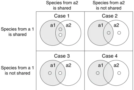
We must first provide a probabilistic derivation of the classic Jaccard and Sørensen incidence indices. Suppose we randomly select a species from Assemblage 1 and a species from Assemblage 2 and then classify each member of the pair according to whether it is a shared species or not. The corresponding probabilities are shown graphically in Fig. 1 and specified in Table 2.
Although the probabilities in Table 2 are not counts, they can be thought of asÔnormalized counts,Õbecause they sum to unity. Substituting these probabilities into eqns 1 and 2, then we have
Jclas¼
A
AþBþC
¼ ½ðS12=S1ÞðS12=S2Þ
½ðS12=S1ÞðS12=S2Þ þ ½ðS12=S1Þð1 ðS12=S2ÞÞ þ ½ð1 ðS12=S1ÞÞðS12=S2Þ ¼ S12
S1þS2S12
which is exactly eqn 3. Likewise, we have
Lclas¼ 2A
2AþBþC
¼ 2½ðS12=S1ÞðS12=S2Þ
2½ðS12=S1ÞðS12=S2Þ þ ½ðS12=S1Þð1 ðS12=S2ÞÞ þ ½ð1 ðS12=S1ÞÞðS12=S2Þ ¼ 2S12
S1þS2
which is the same as eqn 4.
Table 1 Species classification counts used in the classic indices
Assemblage 2
Present Absent
Assemblage 1
Present A B
It might appear that we have made no progress, but this probabilistic approach lays the groundwork for developing abundance-based indices, which in turn allow for the estimation of indices that take into account the effect of unseen shared species. Note that, using this approach, we can also calculate the chance that both randomly chosen species are non-shared species (Case 4 as shown in Fig. 1 and Table 2). However, the basic concept for the Jaccard and Sørensen indices is based only on information for the other three cells (Cases 1–3).
Extending the probabilistic approach to abundance-based indices
Let the probabilities of species discovery (which depend primarily on relative abundance, assuming random mixing and equivalent detectability) in Assemblages 1 and 2 be denoted, respectively, by (p1,p2,…,pS1) and (p1,p2,…,pS2), wherepi> 0,pi> 0 and
PS1
i¼1pi ¼ PSi2¼1pi ¼ 1. We no longer treat all species equally because some species are
common and some are rare. Instead, the basic idea for handling abundance counts is that we treat all individuals equally. Adapting the approach from the previous section, we randomly select one individual from Assemblage 1 and oneindividualfrom Assemblage 2. For each individual of the pair, note whether it belongs to a shared species or not.
We now derive the general formulas for the abundance-based versions of the Jaccard and Sørensen indices. Without loss of generality, we assume the firstS12 species are shared species, that is, the shared species are indexed by 1,2,…,S12. In Assemblage 1, let U denote the total relative abundances of individuals belonging to the shared species,U¼p1+p2+ +pS12. Likewise in Assemblage 2, letVdenote the total relative abundances of individuals belonging to shared species, V¼p1 +p2+ +pS12. Table 3 shows the probabilities that two individuals, one from each assemblage, represent each of the usual four categories.
Based on eqns 1 and 2 for the three probabilities (A, B andCin Table 3), we obtain the following abundance-based indices in terms ofUandV:
Jabd¼ A
AþBþC ¼
UV
UþV UV ð5Þ
a1
a2
Case 1
a1
a2
Case 2
a1
a2
Case 3
a1
a2
Case 4
Species from a 1 is shared
Species from a2 is shared
Species from a 1 is not shared
Species from a2 is not shared Figure 1 A graphical representation of the
meaning of shared species for two assem-blages. Assemblage 1 (a1) is grey, Assem-blage 2 (a2) is white. The grey dot represents a species selected at random from Assem-blage 1 and the white dot represents a species selected at random from Assemblage 2. Case 1 is the only case in which both species are shared species (but not necessar-ily the same species). In Case 2, the species chosen at random from Assemblage 1 is a shared species, but the species chosen from Assemblage 2 is not shared with Assemblage 1. The reverse is true for Case 3. In Case 4, neither of the chosen species is a shared species. These patterns are described mathe-matically in Table 2.
Table 2 Probabilistic derivation of species counts for the classic indices
Select anyspeciesfrom Assemblage 2
Shared Non-shared
Select anyspeciesfrom Assemblage 1 Shared A ¼ S12
S1
S12
S2
(Case 1)
B ¼ S12
S1 1
S12
S2
(Case 2)
Non-shared C ¼ 1 S12
S1
S12
S2
(Case 3)
1 S12
S1
1 S12
S2
(Case 4)
Table 3 Probabilities for individual-based species counts
Select anyindividualfrom Assemblage 2
Shared Non-shared
Select anyindividualfrom Assemblage 1
Shared A¼UV B¼U(1)V)
and
Labd¼
2A 2AþBþC ¼
2UV
U þV ð6Þ
AsUandVrepresent the total abundances of theshared species in Assemblages 1 and 2, respectively, we see that both indices reach 1 for identical assemblages and tend to 0 for disjoint assemblages. In the latter case, for example, Labd¼2/[(1/U) + (1/V)] tends to 0 as both U and V approach 0.
Estimation of the abundance-based indices from sample data
Up to now, we have considered only the species and individuals observed in two assemblages. Both the classic Jaccard and Sørensen and the new, abundance-based versions assume full and complete knowledge of the two assemblages being contrasted. In practice, we need to estimate similarity indices from sample data, the task that we turn to now. Our approach is non-parametric in the sense that we do not need to postulate any particular species abundance distribution to derive the estimators, which are therefore valid under many statistical abundance models (e.g. log-normal, broken stick, gamma, etc.). The derivation does assume that the number of species is finite so that species discovery probabilities are bounded below. [The authors show that the estimators are valid under many of the statistical abundance models (A. Chao, R. L. Chazdon, R. K. Colwell & T.-J. Shen, unpublished data) (e.g. log-normal, exponential, gamma, negative binomial, Zipf– Mandelbrot, broken-stick models, etc.) that appear in Magurran (2004, Table 2.1) or in Plotkin & Muller-Landau (2002, Table 1).]
A random sample ofnindividuals (Sample 1) is taken from Assemblage 1 and a random sample ofmindividuals (Sample 2) is taken from Assemblage 2. Denote the species frequencies in the samples by (X1,X2,…,XS1) and (Y1, Y2, …,YS2), respectively. (Note that if a species is missing from a sample, XiorYiwill equal zero.) Thus, the pair of frequencies for the S12 species truly shared by the two assemblages are (X1,Y1)(X2,Y2)…(XS12,YS12). Assume that D12 of the S12 shared species available are actually observed in both samples, and their frequencies are the first D12 pairs. Thus, an additionalS12 )D12 species are shared by the two assem-blages, but absent from one or both of the samples. The greater the frequencies of rare, shared species observed in one of the two samples, the more probable it is that additional shared species are present in both assemblages, but are absent from one or both samples. We refer to these asunseen shared species.
To incorporate the effect of unseen shared species on the probabilities of Table 3, we use the frequencies ofobserved
rare, shared species to estimate an appropriate adjustment term forUandVto account forunseenshared species. We first define the indicator function I(expression) such that I¼1 ifÔexpressionÕis true andI¼0 ifÔexpressionÕis false. Letf1þ ¼ PDi¼121I X½ i ¼ 1;Yi 1be the observed num-ber ofsharedspecies that are singletons (Xi¼1) in Sample 1 (these species must be present in Sample 2, but may have any abundance). Now, let f2+ be the observed number of shared species that are doubletons (Xi¼2) in Sample 1. Similarly, we definef+1andf+2to be the observed number of shared species that are, respectively, singletons (Yi¼1) and doubletons (Yi¼2) in Sample 2.
Then the proposed estimator forU is
^
U ¼X
D12
i¼1 Xi
n þ
ðm1Þ
m fþ1 2fþ2
XD12
i¼1 Xi
n IðYi ¼1Þ ð7Þ
Notice that the first term in the right-hand side of eqn 7 denotes the observed total of frequencies associated with the observed shared species; the second term accounts for the estimated effect of unseen shared species. Similarly, we have
^
V ¼X
D12
i¼1 Yi
m þ
ðn1Þ
n f1þ 2f2þ
XD12
i¼1 Yi
m IðXi ¼1Þ ð8Þ
When f+2¼0 or f2+¼0, replace f+2 and f2+ in the denominators by f+2+ 1 or f2++ 1, respectively. If the value ofU^ orV^ is greater than 1 (which rarely happens), then it is replaced by 1. Our proposed abundance-based Jaccard and Sørensen estimators are
^ Jabd¼
^ UV^ ^
UþV^ U^V^ ð9Þ
and
^ Labd¼
2U^V^ ^
U þV^ ð10Þ
The variances for these two estimators can be derived by a bootstrap method. (The complete derivation of eqns 7 and 8 and details on the bootstrap procedure for computing variance estimators for eqns 9 and 10 are available upon request from the first author.)
Estimation of similarity indices from incidence frequencies
can be extended to replicated incidence (presence–absence) data.
Suppose we take a set of wreplicated incidence samples from Assemblage X and a set of z replicated incidence samples from Assemblage Y. For both sets of samples combined, there are S species. The number of samples in which a species is found in Assemblage X or Y is the frequencyfor that species in that sample set. The frequencies for speciesi are thus defined as
Xi ¼
Xw
j¼1
xij and Yi ¼
Xz
j¼1 yij;
wherexijandyijrepresent the presence (1) or absence (0) of speciesiin sample j.
Note thatXiorYiwill be zero for some species, unless all species are shared and observed.
Under the assumption that replicate incidence samples are statistically homogeneous (within each assemblage), the chance of a species being present in a particular sample is proportional to its relative abundance in the assemblage, and the frequency vectorsXiorYiare thus statistical proxies for the relative abundance of species in Assemblages XandY (e.g. Chao 2004; Colwell et al. 2004). Thus, with minor changes, eqns 7 and 8 can be used to compute adjusted probabilities that a randomly chosen incidence (species detection) from each of the two assemblages will both represent shared species (though not necessarily the same shared species).
For replicated incidence data,f1+is the number of observed shared species that occur in exactly one sample (Xi¼1) in Xandf2+is the number of observed shared species that occur in exactly two samples (Xi¼2) in X; f+1 and f+2 are the corresponding numbers for sample matrix Y. Define the sum of the incidence frequencies for the matrices as
n¼X
S
i¼1
Xi and m¼
XS
i¼1 Yi:
Then the proposed estimators are
^
Uinc¼X D12
i¼1 Xi
n þ
z1
ð Þ
z fþ1 2fþ2
XD12
i¼1 Xi
n I Yð i ¼1Þ
ð11Þ
and
^ Vinc¼
XD12
i¼1 Yi
m þ
w1
ð Þ
w f1þ 2f2þ
XD12
i¼1 Yi
mI Xð i ¼1Þ
ð12Þ
(The same modifications described for eqns 7 and 8 may be applied here if f+2¼0 or f2+¼0.) Thus, our proposed incidence-based Jaccard and Sørensen estimators are
^ Jinc¼
^ UincV^inc ^
UincþV^incU^incV^inc
ð13Þ
and
^ Linc¼
2U^incV^inc ^
UincþV^inc
: ð14Þ
P E R F O R M A N C E T E S T S : C L A S S I C V S . N E W I N D I C E S
Indices tested
We carried out performance tests for: (1) the classic Jaccard and Sørensen indices (eqns 1 and 2); (2) the new, abundance-based Jaccard and Sørensen indices (eqns 5 and 6); (3) the estimators for the abundance-based indices (eqns 9 and 10); and (4) the replicated-incidence estimators for the abundance-based indices (eqns 13 and 14).
Data sets used in the tests
We conducted the performance tests on a large, species-rich data set for tropical rainforest ants (Longino et al. 2002), collected using several replicated, mass-collecting techniques at La Selva Biological Station in Costa Rica. Here, we present representative results for three collection methods: Berlese extraction of soil samples (217 samples, 4318 individuals, 117 species, of which 19 were singletons), Malaise trap samples for flying and crawling insects (62 samples, 1660 individuals, 103 species, of which 35 were singletons), and Fogging samples from canopy fogging (459 samples, 26302 individuals, 165 species of which 19 were singletons). [Relative abundance diagrams appear in Longinoet al.(2002).] As Longinoet al. (2002) point out, these three methods intentionally sample different, but overlapping segments of the local ant fauna. Whereas the raw species sum for the three methods would be 117 + 103 + 165¼385 species, the actual number of species captured by the three methods together was only 276 species. Parallel tests for other high-richness data sets, including the rainforest tree data discussed later in this paper, yielded concordant results (A. Chao, R. L. Chazdon, R. K. Colwell & T.-J. Shen, unpublished data).
The tests
Nevertheless, indices of compositional similarity can be compared in terms of their performance in tests of sensitivity to undersampling. Using the ant data, we illustrate three tests: (1) Test 1: equal-sized samples from a single data set (within-assemblage rarefaction); (2) Test 2: unequal-sized samples from a single data set; and (3) Test 3: equal-proportion samples from two data sets (between-assemblage rarefaction). For purposes of these tests, we treated the ant data from each collecting method (Berlese, Malaise, or Fogging) as a separate, complete Ôassemblage,Õ referred to here as asampling pool. Samples of specified sizes (in terms of numbers of individuals) were then selected, at random,with replacement, from these pools. Of course, not all species present in a sampling pool are represented in smaller samples. However, because sampling was done with replacement, not all species are present even when the number of individuals selected is the same as the number of individuals in the pool.
R E S U L T S
Test 1: Equal-sized samples from a single data set
All similarity indices yield a true value of 1 when a complete sampling pool (assemblage) is compared with itself. What happens when a similarity index is computed for two
random samples of a single sampling pool? If an index is unbiased by sample size, it should yield a value of 1 when applied to samples of any size. First, we randomly sampled individuals (with replacement) from the pooled ant data for a single collecting method to produce pairs of samples having the same number of individuals as the pools themselves (full samples). Next, we randomly selected smaller samples, each totalling one-half the number of individuals in the original sampling pool, then computed similarity indices for this sample pair. We then repeated this procedure for a pair of samples each 1/4 the size of the original pool, then a pair 1/8 the size of the pool, and so on, successively halving sample size, down to 1/64 the original number of individuals. (Note that this is quite a severe test of undersampling bias, even for these very large pools.) This entire process was repeated 1000 times and means taken, for each test of each index, and for each of the three ant collecting methods.
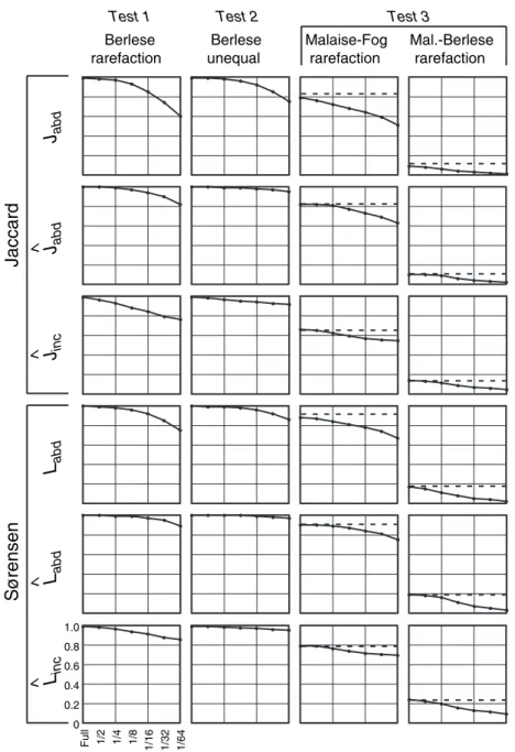
Figure 2 shows representative results of this test for the classic Jaccard and Sørensen indices (first column of panels, Test 1: Berlese rarefaction). Clearly both of these indices were quite sensitive to undersampling. Figure 3 (first column of panels) shows the corresponding results for the new indices for this test. The new abundance-based Jaccard and Sørensen indices, without adjustment for unseen shared species (JabdandLabd), were also sensitive to sample size. In
Berlese rarefaction
Berlese unequal
Malaise-Fog rarefaction
Mal.-Berlese rarefaction
1/2 1/4 1/8 1/16 1/32 1/64
Full
0 0.2 0.4 0.6 0.8 1.0
J
clasL
clasJaccard
Sørensen
Test 1 Test 2 Test 3
Berlese rarefaction
Berlese unequal
Malaise-Fog rarefaction
Mal.-Berlese rarefaction
1/2 1/4 1/8 1/16 1/32 1/64
Full
0 0.2 0.4 0.6 0.8 1.0
J
abd^ J
abdJ
inc^
L
abd^ L
abdL
inc^
Jaccard
Sørensen
Test 1 Test 2 Test 3
contrast, the Jaccard and Sørensen estimators, which include the estimated effect of unseen shared species, proved to be less sensitive to undersampling, remaining substantially closer to 1 even for small samples (Fig. 3). This was true for both the abundance-based estimators (^JabdandL^abd) and the estimators based on replicated incidence data (^Jinc and ^
Linc).
Test 2: Unequal-sized samples from a single data set
A similarity index should ideally be robust to sample size not only for equal-sized samples, but also for samples of unequal size. To test for this property we computed similarity indices for samples of successively smaller size, vs.
ÔfullÕsamples, equal in number of individuals to the number in the corresponding sampling pool. As with the first test, an ideal index should remain at 1, regardless of the discrepancy in sample sizes. Figures 2 and 3 (second column, Test 2: Berlese unequal) show such a test for the Berlese sample ant data, using samples created by the same scheme outlined for the first method. Even more than in the first test, the classic Jaccard and Sørensen indices (Fig. 2) were strongly affected by the size of the sample, leading to a severe negative bias when one sample was markedly smaller than the full sample. In contrast, the new Jaccard and Sørensen estimators (Fig. 3, second column) were strikingly resistant to undersampling, including both abundance-based estima-tors (^Jabd andL^abd) and the estimators based on replicated incidence data (^Jinc andL^inc).
Equal-proportion samples from two data sets
It is all very well for a similarity index to be robust to sample size in comparing paired samples from the same pool, but an index is of little use if it does not retain that robustness in comparing different data sets, while successfully detecting compositional differences between them. We performed the same sample size comparison procedures described for the first set of tests, but instead of comparing sample pairs from the same sampling pool, we compared successively smaller sample pairs from the Malaise and Fogging [high similarity (Longino et al. 2002)], and from the Malaise and Berlese (low similarity) data sets. The results for the classic Jaccard and Sørensen indices appear in the third and fourth columns of Fig. 2. An ideal index would yield and maintain the true value computed for the full pools (the dotted horizontal line in each panel) in the face of rarefaction. The classic Jaccard and Sørensen indices proved quite sensitive to undersam-pling in this test (Fig. 2). The new abundance-based Jaccard and Sørensen indices, uncorrected for unseen species (Jabd andLabdin third and fourth columns of Fig. 3), also suffer from undersampling bias, but the bias is quite substantially reduced for their abundance-based counterparts corrected
for unseen species (^Jabd and L^abd in third and fourth columns of Fig. 3) as well as for the corresponding estimators based on replicated incidence data (^Jinc andL^inc in third and fourth columns of Fig. 3).
A P P L I C A T I O N
As an example of the application of the new indices, we apply the classic Jaccard index (eqn 1), the new abundance-based Jaccard index (eqn 5) and its estimator (eqn 9) to data from two mature and four second-growth rainforest sites in Costa Rica. We examine compositional similarity between species of trees ‡25 cm diameter at breast height (DBH; canopy individuals), canopy tree saplings (1–5 cm DBH) and canopy tree seedlings (> 20 cm height, but < 1 cm DBH) within four second-growth forests of different age since pasture abandonment and in two old-growth forests in the same study area. During early stages of succession, when the forest canopy is first beginning to close, fast-growing, shade-intolerant colonizing tree species are present as canopy trees and are also found as smaller individuals in the understory, as seedlings and saplings. As time progresses and the understory becomes more shaded, these shade-intolerant tree species are eliminated from the seedling and sapling pool and shade-tolerant species readily colonize these small size classes. These shade-tolerant species are represented by seedlings and saplings, but have few or no canopy trees present, gradually augmenting tree species richness as the forest matures (Guariguata et al. 1997; Table 4). Thus, we would predict that, as secondary forests mature, compositional similarity between tree species
Table 4 Observed patterns of species richness of tree seedlings, saplings and canopy individuals in 1 ha plots in four second-growth and two old-second-growth forests in year 2000
Site Age
Sobs seedlings
Sobs saplings
Sobs canopy trees
LSUR 15 45 68 12
TIR 18 49 74 16
LEP 23 47 67 24
CR 28 57 91 33
LSUR old-growth > 200 47 101 37 LEP old-growth > 200 69 102 43
and seedlings or saplings would initially be high, but would quickly decline to a minimum during intermediate stages of succession and then begin to increase later in succession as shade-tolerant trees reach reproductive maturity and pro-duce seedlings that can establish, grow and survive.
The classic Jaccard index (eqn 1) showed low compo-sitional similarity between trees and seedlings for the four second-growth forests compared with the old-growth forests, with similarity decreasing slightly with age among the four second-growth forests (Fig. 4). Similarity between trees and saplings, in contrast, showed gradual increases from the youngest forest to the older second-growth forest, continuing the trend to old-growth forests (Fig. 4).
The abundance-based Jaccard index (eqn 5) showed a strikingly different pattern across the six forest stands. Compositional similarity between seedling and tree assem-blages and between sapling and tree assemassem-blages was initially high in the youngest stand, as we had predicted. As the forest matures, tree seedling and sapling pools become enriched by shade-tolerant species not represented as canopy trees, resulting in a decreasing compositional similarity that reached a minimum in the 23-year-old LEP stand (Fig. 4). This minimum similarity represents a point in forest succession of maximum recruitment limitation for both seedlings and saplings. In the oldest second-growth plot, CR, the abundance-based Jaccard index began to increase, reflecting recruitment of shade-tolerant species in all three-size classes (Fig. 4). The similarity index continued to increase and stabilized at 0.4–0.5 in the two old-growth stands. With the exception of one old-growth stand, similarity indices were higher for seedlings vs. trees than for saplings vs. trees. At the scale of 1 ha plots, compositional similarity between canopy trees and seedling and sapling size classes in old-growth forests was comparable to that observed within a 15-year-old second-growth forest, but greater than that observed in second-growth forests of intermediate age. By design, the abundance-based Jaccard index responds sensitively to changes in total relative abundances of shared species during forest succession.
The abundance-based Jaccard estimator (eqn 9), which incorporates the effects of unseen shared species, showed similar general trends across stands when compared with the abundance-based Jaccard index (Fig. 4). The 28-year-old second-growth stand, however, had nearly comparable estimates of similarity compared with the two old-growth stands, suggesting that the estimator is responding to rare or infrequent species that are shared between the size classes (Fig. 4). The estimator for sapling vs. tree similarity was higher than for seedling vs. trees in the TIR second-growth site, indicating that this stand has more rare species of shared saplings than seedlings.
C O N C L U S I O N S
Becausesimilarityis a qualitative human construct, it has no precise mathematical definition. Nevertheless, measuring
ÔsimilarityÕ relies on quantitative indices devised for the purpose, and in practice, we may expect that similarity indices fulfil reasonable criteria for their mathematical behaviour (Legendre & Legendre 1998). Given indices that make sense mathematically, it is their statistical performance under the realities of field sampling that we have concerned ourselves with here, particularly for species-rich taxa for which complete inventories are impractical or even impossible.
0.1 0.2 0.3
0
0.1 0.2 0.3 0.4 0.5
0
0.1 0.2 0.3 0.4 0.5
0
LSUR TIR LEP CR LSUR LEP Forest site
15 18 23 28 Old growth Forest age (year)
Jabd
^ Jabd Jclas
Seedlings vs.trees
Saplings vs.trees
0.6 0.7
Using sampling simulations applied to representative field data sets, we confirmed that two of the most widely used classic indices, Jaccard and Sørensen, are negatively biased under conditions of undersampling, often quite substantially (Fig. 2). Our objective was to develop new, probability-based indices that reduce undersampling bias by estimating and compensating for the effects of unseen, shared species. We based a new similarity index on the probability that two randomly chosen individuals, one from each of two samples, both belong to any of the species shared by the two samples [not necessarily to the same shared species, the basis ofF(Chave & Leigh 2002; Condit et al. 2002) and the Morisita–Horn index]. This approach opened the way to the crucial step, adjusting this probability to account for the chance that larger samples would reveal a larger proportion of shared species. As anticipated, the new indices consistently reduced undersampling bias in the per-formance tests, in most circumstances quite substantially. Inevitably some bias remains, especially under severe undersampling and for highly dissimilar samples. Under such conditions, relatively little information exists to guide bias reduction.
Ecologists distinguish two aspects of the compositional similarity of species assemblages: similarity of species lists (incidence) and similarity of speciesÕ relative abundances. Classic abundance-based indices (e.g. Morisita–Horn or Bray–Curtis) match abundances, species-by-species. Our new indices take an intermediate path, by assessing the probability that individuals belong to shared vs. unshared species, without regard to which species they belong to. Unfortunately for many studies, unreplicated, pure incidence data (pairs of species lists) provide no information that can be used to estimate the number of unseen, shared species. In principle, it may be possible to derive estimators that use abundance data to correct pure incidence similarity indices for unseen species, but it is currently statistically difficult for biologically realistic data. However, we recommend the new indices for any application in which not only species matching but similarity of relative abundance is of interest. Moreover, these new indices are better suited than the corresponding classic indices for assessing compositional similarity between samples that differ in size, are known or suspected to be undersampled, or are likely to contain numerous rare species.
A C K N O W L E D G E M E N T S
We thank three anonymous referees for their comments and suggestions. This work was supported by Taiwan National Science Council Contract NSC92-2118-M007-013 to A. Chao and T.-J. Shen, by a grant from the Andrew W. Mellon Foundation to R. L. Chazdon, and by US-NSF grant DEB-0072702 to R. K. Colwell. We thank Jorge Leiva
for sharing vegetation data for tree species in mature forests. The new estimators presented in this paper are included in version 7.5 of ESTIMATES (Colwell 2004) and the program SPADE(Chao & Shen 2003), to be released upon publication of this paper. The complete derivation of eqns 7 and 8 and the variance estimators for eqns 9 and 10 are available upon request from the first author. The complete ant data sets are available from RKC.
R E F E R E N C E S
Arita, H.T. & Rodrı´guez, P. (2002). Geographic range, turnover rate and the scaling of species diversity.Ecography, 25, 541–550. Arita, H.T. & Rodrı´guez, P. (2004). Local–regional relationships and the geographical distribution of species.Global Ecol. Biogeogr., 13, 15–21.
Balvanera, P., Lott, E., Segura, G., Siebe, C. & Islas, A. (2002). Beta diversity patterns and correlates in a tropical dry forest of Mexico.J. Veg. Sci., 13, 145–158.
Bray, J.R. & Curtis, J.T. (1957). An ordination of the upland forest communities of southern Wisconsin.Ecol. Monogr., 27, 325–349. Bunge, J. & Fitzpatrick, M. (1993). Estimating the number of
species: a review.J. Am. Stat. Assoc., 88, 364–373.
Chao, A. (in press). Species richness estimation. In:Encyclopedia of Statistical Sciences, 2nd edn (eds Balakrishnan, N., Read, C.B. & Vidakovic, B.). Wiley Press, New York, NY, USA.
Chao, A. & Shen, T.J. (2003). ProgramSPADE(Species Prediction and Diversity Estimation). Program and User’s Guide available at http://chao.stat.nthu.edu.tw.
Chao, A., Ma, M.-C. & Yang, M.C.K. (1993). Stopping rules and estimation for recapture debugging with unequal failure rates. Biometrika, 80, 193–201.
Chave, J. & Leigh, E.G. (2002). A spatially explicit neutral model of beta-diversity in tropical forests.Theor. Pop. Biol., 62, 153–168. Chazdon, R.L., Colwell, R.K., Denslow, J.S. & Guariguata, M.R.
(1998). Statistical methods for estimating species richness of woody regeneration in primary and secondary rain forests of NE Costa Rica. In:Forest Biodiversity Research, Monitoring and Modeling: Conceptual Background and Old World Case Studies. (eds Dallmeier, F. & Comiskey, J.). Parthenon Publishing, Paris, France, pp. 285–309.
Colwell, R.K. (2004).ESTIMATES: Statistical Estimation of Species Richness and Shared Species from Samples, Version 7.5. Available at http://viceroy.eeb.uconn.edu/estimates. Persistent URL http://purl.oclc.org/estimates.
Colwell, R.K. & Coddington, J.A. (1994). Estimating terrestrial biodiversity through extrapolation.Phil. Trans. R. Soc. Lond. B Biol. Sci., 345, 101–118.
Colwell, R.K., Mao, C.X. & Chang, J. (2004). Interpolating, extrapolating, and comparing incidence-based species accumu-lation curves.Ecology, 85, 2717–2727.
Condit, R., Pitman, N., Leigh, E.G., Jr, Chave, J., Terborgh, J., Foster, R.B.et al.(2002). Beta-diversity in tropical forest trees. Science, 295, 666–669.
Duivenvoorden, J.F. (1995). Tree species composition and rain forest-environment relationships in the middle Caqueta´ area, Colombia, NW Amazonia.Vegetatio, 120, 91–113.
Fisher, B.L. (1999). Improving inventory efficiency: a case study of leaf-litter ant diversity in Madagascar. Ecol. Appl., 9, 714– 731.
Grassle, J.F. & Smith, W. (1976). A similarity measure sensitive to the contribution of rare species and its use in investigation of variation in marine benthic communities.Oecologia, 25, 13–22. Guariguata, M.R., Chazdon, R.L., Denslow, J.S., Dupuy, J.M.,
Anderson, L. (1997). Structure and floristics of secondary and old-growth forest stands in lowland Costa Rica. Plant Ecology, 132, 107–120.
Harte, J., Kinzig, A. & Green, J. (1999). Self-similarity in the dis-tribution and abundance of species.Science, 284, 334–336. Hubbell, S.P. (2001). A Unified Neutral Theory of Biodiversity and
Biogeography. Princeton University Press, Princeton, NJ. Koleff, P., Gaston, K.J. & Lennon, J.J. (2003). Measuring beta
diversity for presence–absence data.J. Anim. Ecol., 72, 367–382. Lee, S.-M. & Chao, A. (1994). Estimating population size via sample coverage for closed capture–recapture models.Biometrics, 50, 88–97.
Legendre, P. & Legendre, L. (1998). Numerical Ecology. Elsevier, Amsterdam.
Leigh, E.G., Wright, S.J., Putz, F.E. & Herre, E.A. (1993). The decline of tree diversity on newly isolated tropical islands: a test of a null hypothesis and some implications. Evol. Ecol., 7, 76– 102.
Lennon, J.J., Koleff, P., Greenwood, J.J.D. & Gaston, K.J. (2001). The geographical structure of British bird distributions: diversity, spatial turnover and scale.J. Anim. Ecol., 70, 966–979.
Longino, J.T., Coddington, J. & Colwell, R.K. (2002). The ant fauna of a tropical rain forest: estimating species richness three different ways.Ecology, 83, 689–702.
MacKenzie, D.I., Bailey, L.L. & Nichols, J.D. (2004). Investigating species co-occurrence patterns when species are detected im-perfectly.J. Anim. Ecol., 73, 546–555
Magurran, A.E. (2004). Measuring Biological Diversity. Blackwell, Oxford.
Plotkin, J.B. & Muller-Landau, H.C. (2002). Sampling the species composition of a landscape.Ecology, 83, 3344–3356.
Rodrı´guez, P. & Arita, H.T. (2004). Beta diversity and latitude in North American mammals: testing the hypothesis of covaria-tion.Ecography, 27, 1–11.
Ruokolainen, K. & Tuomisto, H. (2002). Beta-diversity in tropical forests.Science, 297, 1439a.
Valencia, R., Foster, R.B., Villa, G., Condit, R., Svenning, J.-C., Herna´ndez, C.et al.(2004). Tree species distributions and local habitat variation in the Amazon: large forest plot in eastern Ecuador.J. Ecol., 92, 214–229
Wolda, H. (1981). Similarity indices, sample size and diversity. Oecologia, 50, 296–302.
Editor, Nicholas Gotelli