21 The Kinetic Theory of Gases pdf

During periods of strenuous exertion, our bodies generate excess internal energy that must be released into our surround-ings. To facilitate this release, humans perspire. Dogs and other animals pant to accomplish the same goal. Both actions involve the evaporation of a liquid. How does this process help cool the body?

(Photograph of runner by Jim Cummins/FPG International; photograph of beagle by Renee Lynn/Photo Researchers, Inc.)

The Kinetic Theory of Gases

C h a p t e r O u t l i n e

21.1 Molecular Model of an Ideal Gas

21.2 Molar Specific Heat of an Ideal Gas

21.3 Adiabatic Processes for an Ideal Gas

21.4 The Equipartition of Energy

21.5 The Boltzmann Distribution Law

21.6 Distribution of Molecular Speeds

21.7 (Optional)Mean Free Path

c

h

a

p

t

e

r

21.1 Molecular Model of an Ideal Gas 641

n Chapter 19 we discussed the properties of an ideal gas, using such macro-scopic variables as pressure, volume, and temperature. We shall now show that such large-scale properties can be described on a microscopic scale, where mat-ter is treated as a collection of molecules. Newton’s laws of motion applied in a sta-tistical manner to a collection of particles provide a reasonable description of ther-modynamic processes. To keep the mathematics relatively simple, we shall consider molecular behavior of gases only, because in gases the interactions be-tween molecules are much weaker than they are in liquids or solids. In the current view of gas behavior, called the kinetic theory,gas molecules move about in a ran-dom fashion, colliding with the walls of their container and with each other. Per-haps the most important feature of this theory is that it demonstrates that the ki-netic energy of molecular motion and the internal energy of a gas system are equivalent. Furthermore, the kinetic theory provides us with a physical basis for our understanding of the concept of temperature.

In the simplest model of a gas, each molecule is considered to be a hard sphere that collides elastically with other molecules and with the container’s walls. The hard-sphere model assumes that the molecules do not interact with each other except during collisions and that they are not deformed by collisions. This description is adequate only for monatomic gases, for which the energy is entirely translational kinetic energy. One must modify the theory for more complex mole-cules, such as oxygen (O2) and carbon dioxide (CO2), to include the internal

en-ergy associated with rotations and vibrations of the molecules.

MOLECULAR MODEL OF AN IDEAL GAS

We begin this chapter by developing a microscopic model of an ideal gas. The model shows that the pressure that a gas exerts on the walls of its container is a consequence of the collisions of the gas molecules with the walls. As we shall see, the model is consistent with the macroscopic description of Chapter 19. In devel-oping this model, we make the following assumptions:

• The number of molecules is large, and the average separation between mole-cules is great compared with their dimensions. This means that the volume of the molecules is negligible when compared with the volume of the container.

• The molecules obey Newton’s laws of motion, but as a whole they move ran-domly. By “randomly” we mean that any molecule can move in any direction with equal probability. We also assume that the distribution of speeds does not change in time, despite the collisions between molecules. That is, at any given moment, a certain percentage of molecules move at high speeds, a certain per-centage move at low speeds, and a certain perper-centage move at speeds intermedi-ate between high and low.

• The molecules undergo elastic collisions with each other and with the walls of the container. Thus, in the collisions, both kinetic energy and momentum are constant.

• The forces between molecules are negligible except during a collision. The forces between molecules are short-range, so the molecules interact with each other only during collisions.

• The gas under consideration is a pure substance. That is, all of its molecules are identical.

Although we often picture an ideal gas as consisting of single atoms, we can as-sume that the behavior of molecular gases approximates that of ideal gases rather

21.1

I

10.5

well at low pressures. Molecular rotations or vibrations have no effect, on the aver-age, on the motions that we considered here.

Now let us derive an expression for the pressure of an ideal gas consisting of N molecules in a container of volume V. The container is a cube with edges of length d(Fig. 21.1). Consider the collision of one molecule moving with a velocity v to-ward the right-hand face of the box. The molecule has velocity components vx, vy,

and vz. Previously, we used m to represent the mass of a sample, but throughout

this chapter we shall use mto represent the mass of one molecule. As the molecule collides with the wall elastically, its xcomponent of velocity is reversed, while its y and z components of velocity remain unaltered (Fig. 21.2). Because the x compo-nent of the momentum of the molecule is mvxbefore the collision and ⫺mvxafter

the collision, the change in momentum of the molecule is

Applying the impulse – momentum theorem (Eq. 9.9) to the molecule gives

where F1is the magnitude of the average force exerted by the wall on the

mole-cule in the time ⌬t. The subscript 1 indicates that we are currently considering only one molecule. For the molecule to collide twice with the same wall, it must travel a distance 2din the x direction. Therefore, the time interval between two collisions with the same wall is Over a time interval that is long com-pared with ⌬t, the average force exerted on the molecule for each collision is

(21.1)

According to Newton’s third law, the average force exerted by the molecule on the wall is equal in magnitude and opposite in direction to the force in Equation 21.1:

Each molecule of the gas exerts a force F1on the wall. We find the total force F

ex-erted by all the molecules on the wall by adding the forces exex-erted by the individ-ual molecules:

In this equation, vx1is the xcomponent of velocity of molecule 1, vx2is the x

com-ponent of velocity of molecule 2, and so on. The summation terminates when we reach Nmolecules because there are Nmolecules in the container.

To proceed further, we must note that the average value of the square of the velocity in the xdirection for Nmolecules is

Thus, the total force exerted on the wall can be written

Now let us focus on one molecule in the container whose velocity components are vx, vy, and vz. The Pythagorean theorem relates the square of the speed of this

F⫽ Nm d vx

2

vx2⫽

vx12⫹vx22⫹ ⭈⭈⭈ ⫹vxN2

N F⫽ m

d (vx1

2_⫹v

x22⫹ ⭈⭈⭈)

F1, on wall⫽ ⫺F1⫽ ⫺

冢

⫺mvx2

d

冣

⫽

mvx2

d F1⫽

⫺2mvx

⌬t ⫽

⫺2mvx

2d/vx ⫽

⫺mvx2

d

⌬t⫽2d/vx.

F1⌬t⫽ ⌬px⫽ ⫺2mvx

⌬px⫽ ⫺mvx⫺(mvx)⫽ ⫺2mvx d

d d

z _x

y

m

v

v_x

Figure 21.1 A cubical box with sides of length dcontaining an ideal gas. The molecule shown moves with velocity v.

Figure 21.2 A molecule makes an elastic collision with the wall of the container. Its xcomponent of momentum is reversed, while its y

component remains unchanged. In this construction, we assume that the molecule moves in the xy

plane. vy

vx

v vy

–vx

21.1 Molecular Model of an Ideal Gas 643

molecule to the squares of these components:

Hence, the average value of v2for all the molecules in the container is related to the average values of vx2, vy2, and vz2according to the expression

Because the motion is completely random, the average values and are equal to each other. Using this fact and the previous equation, we find that

Thus, the total force exerted on the wall is

Using this expression, we can find the total pressure exerted on the wall:

(21.2)

This result indicates that the pressure is proportional to the number of mole-cules per unit volume and to the average translational kinetic energy of the molecules, In deriving this simplified model of an ideal gas, we obtain an important result that relates the large-scale quantity of pressure to an atomic quan-tity — the average value of the square of the molecular speed. Thus, we have estab-lished a key link between the atomic world and the large-scale world.

You should note that Equation 21.2 verifies some features of pressure with which you are probably familiar. One way to increase the pressure inside a con-tainer is to increase the number of molecules per unit volume in the concon-tainer. This is what you do when you add air to a tire. The pressure in the tire can also be increased by increasing the average translational kinetic energy of the air mole-cules in the tire. As we shall soon see, this can be accomplished by increasing the temperature of that air. It is for this reason that the pressure inside a tire increases as the tire warms up during long trips. The continuous flexing of the tire as it moves along the surface of a road results in work done as parts of the tire distort and in an increase in internal energy of the rubber. The increased temperature of the rubber results in the transfer of energy by heat into the air inside the tire. This transfer increases the air’s temperature, and this increase in temperature in turn produces an increase in pressure.

Molecular Interpretation of Temperature

We can gain some insight into the meaning of temperature by first writing Equa-tion 21.2 in the more familiar form

Let us now compare this with the equation of state for an ideal gas (Eq. 19.10):

PV⫽NkBT

PV⫽2₃N

冢

1₂mv2

冣

1 2mv2.

P⫽ 2 3

冢

N V

冣冢

1 2 mv

2

冣

P⫽ F

A ⫽

F d2 ⫽

1 3

冢

N d3 mv

2

冣

_⫽ 1

3

冢

N V

冣

mv

2

F⫽ N 3

冢

mv2

d

冣

v2_⫽3v

x2

vz2

vy2,

vx2,

v2_⫽v

x2⫹vy2⫹vz2

v2_⫽v

x2⫹vy2⫹vz2

Ludwig Boltzmann

Austrian theoretical physicist (1844 – 1906)

Boltzmann made many important con-tributions to the development of the kinetic theory of gases, electromag-netism, and thermodynamics. His pio-neering work in the field of kinetic theory led to the branch of physics known as statistical mechanics.

(Courtesy of AIP Niels Bohr Library, Lande Collection)

Relationship between pressure and molecular kinetic energy

Recall that the equation of state is based on experimental facts concerning the macroscopic behavior of gases. Equating the right sides of these expressions, we find that

(21.3)

That is, temperature is a direct measure of average molecular kinetic energy.

By rearranging Equation 21.3, we can relate the translational molecular ki-netic energy to the temperature:

(21.4)

That is, the average translational kinetic energy per molecule is Because it follows that

(21.5)

In a similar manner, it follows that the motions in the yand zdirections give us

Thus, each translational degree of freedom contributes an equal amount of en-ergy to the gas, namely, (In general, “degrees of freedom” refers to the num-ber of independent means by which a molecule can possess energy.) A generaliza-tion of this result, known as the theorem of equipartition of energy,states that

1 2kBT. 1

2mvy2⫽12kBT

and

12mvz2⫽12kBT 1

2mvx2⫽12kBT

vx2⫽13v2,

3 2kBT. 1

2mv2⫽ 3 2kBT

T⫽ 2

3kB

冢

1 2mv2

冣

each degree of freedom contributes 1₂kBT to the energy of a system.

Temperature is proportional to average kinetic energy

Average kinetic energy per molecule

Theorem of equipartition of energy

Total translational kinetic energy of Nmolecules

The total translational kinetic energy of Nmolecules of gas is simply Ntimes the average energy per molecule, which is given by Equation 21.4:

(21.6)

where we have used for Boltzmann’s constant and for the

number of moles of gas. If we consider a gas for which the only type of energy for the molecules is translational kinetic energy, we can use Equation 21.6 to express

n⫽N/NA

kB⫽R/NA

Etrans⫽N

冢

12mv2

冣

⫽ 3

2NkBT⫽32nRT

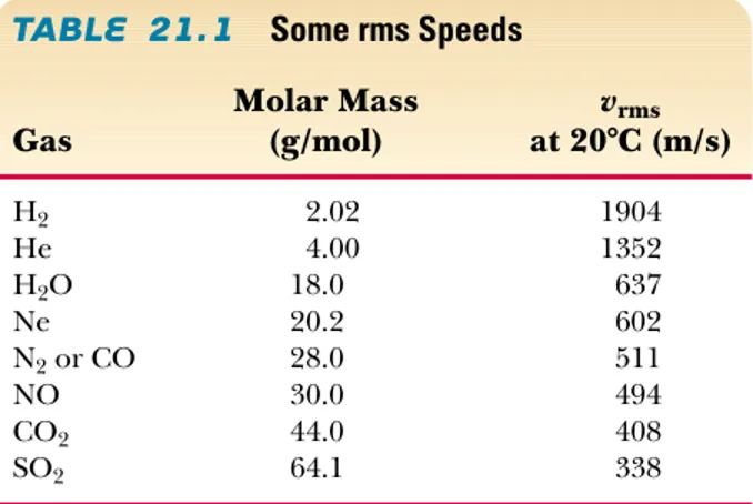
TABLE 21.1

Some rms Speeds

Molar Mass vrms

Gas (g/mol) at 20°C (m/s)

H2 2.02 1904

He 4.00 1352

H2O 18.0 637

Ne 20.2 602

N2or CO 28.0 511

NO 30.0 494

CO2 44.0 408

21.2 Molar Specific Heat of an Ideal Gas 645

the internal energy of the gas. This result implies that the internal energy of an ideal gas depends only on the temperature.

The square root of is called the root-mean-square (rms) speed of the mole-cules. From Equation 21.4 we obtain, for the rms speed,

(21.7)

where Mis the molar mass in kilograms per mole. This expression shows that, at a given temperature, lighter molecules move faster, on the average, than do heavier molecules. For example, at a given temperature, hydrogen molecules, whose mo-lar mass is 2⫻10⫺3kg/mol, have an average speed four times that of oxygen mol-ecules, whose molar mass is 32⫻10⫺3kg/mol. Table 21.1 lists the rms speeds for various molecules at 20°C.

vrms⫽

!

v2⫽

!

3kBT

m ⫽

!

3RT M v2

At room temperature, the average speed of an air molecule is several hundred meters per second. A molecule traveling at this speed should travel across a room in a small fraction of a second. In view of this, why does it take the odor of perfume (or other smells) several minutes to travel across the room?

MOLAR SPECIFIC HEAT OF AN IDEAL GAS

The energy required to raise the temperature of n moles of gas from Tito Tf

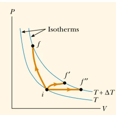
de-pends on the path taken between the initial and final states. To understand this, let us consider an ideal gas undergoing several processes such that the change in temperature is for all processes. The temperature change can be achieved by taking a variety of paths from one isotherm to another, as shown in Figure 21.3. Because ⌬Tis the same for each path, the change in internal energy ⌬Eint is the same for all paths. However, we know from the first law,

that the heat Q is different for each path because W(the area un-der the curves) is different for each path. Thus, the heat associated with a given change in temperature does not have a unique value.

Q⫽ ⌬Eint⫹W,

⌬T⫽Tf⫺Ti

21.2

Quick Quiz 21.1

Root-mean-square speed

A Tank of Helium

E

XAMPLE

21.1

Solution

Using Equation 21.4, we find that the average ki-netic energy per molecule is

Exercise

Using the fact that the molar mass of helium is 4.00⫻10⫺3_{kg/mol, determine the rms speed of the atoms}

at 20.0°C.

Answer

1.35⫻103_m/s.

6.07⫻10⫺21 _J ⫽

1 2mv2⫽

3

2kBT⫽32(1.38⫻10⫺23 J/K)(293 K)

A tank used for filling helium balloons has a volume of 0.300 m3_{and contains 2.00 mol of helium gas at 20.0°C.}

Assum-ing that the helium behaves like an ideal gas, (a) what is the total translational kinetic energy of the molecules of the gas?

Solution

Using Equation 21.6 with mol and 293 K, we find that

(b) What is the average kinetic energy per molecule? 7.30⫻103 _J

⫽

Etrans⫽32nRT⫽ 3

2(2.00 mol)(8.31 J/mol⭈K)(293 K)

T⫽

n⫽2.00

P

V

Isotherms

i f

f ′

T + ∆T

f ′′

T

Figure 21.3 An ideal gas is taken from one isotherm at temperature

Tto another at temperature along three different paths.

T⫹ ⌬T

We can address this difficulty by defining specific heats for two processes that frequently occur: changes at constant volume and changes at constant pressure. Because the number of moles is a convenient measure of the amount of gas, we define the molar specific heatsassociated with these processes with the following equations:

(constant volume) (21.8)

(constant pressure) (21.9)

where CV is the molar specific heat at constant volume and CP is the molar

specific heat at constant pressure.When we heat a gas at constant pressure, not only does the internal energy of the gas increase, but the gas also does work be-cause of the change in volume. Therefore, the heat Qconstant P must account for

both the increase in internal energy and the transfer of energy out of the system by work, and so Qconstant Pis greater than Qconstant V. Thus, CPis greater than CV.

In the previous section, we found that the temperature of a gas is a measure of the average translational kinetic energy of the gas molecules. This kinetic energy is associated with the motion of the center of mass of each molecule. It does not in-clude the energy associated with the internal motion of the molecule — namely, vi-brations and rotations about the center of mass. This should not be surprising be-cause the simple kinetic theory model assumes a structureless molecule.

In view of this, let us first consider the simplest case of an ideal monatomic gas, that is, a gas containing one atom per molecule, such as helium, neon, or ar-gon. When energy is added to a monatomic gas in a container of fixed volume (by heating, for example), all of the added energy goes into increasing the transla-tional kinetic energy of the atoms. There is no other way to store the energy in a monatomic gas. Therefore, from Equation 21.6, we see that the total internal en-ergy Eintof Nmolecules (or n mol) of an ideal monatomic gas is

(21.10)

Note that for a monatomic ideal gas, Eintis a function of Tonly, and the functional

relationship is given by Equation 21.10. In general, the internal energy of an ideal gas is a function of Tonly, and the exact relationship depends on the type of gas, as we shall soon explore.

How does the internal energy of a gas change as its pressure is decreased while its volume is increased in such a way that the process follows the isotherm labeled T in Figure 21.4? (a) Eintincreases. (b) Eintdecreases. (c) Eintstays the same. (d) There is not enough

infor-mation to determine ⌬Eint.

If energy is transferred by heat to a system at constant volume,then no work is done by the system. That is, for a constant-volume process. Hence, from the first law of thermodynamics, we see that

(21.11)

In other words, all of the energy transferred by heat goes into increasing the in-ternal energy (and temperature) of the system. A constant-volume process from i to fis described in Figure 21.4, where ⌬Tis the temperature difference between the two isotherms. Substituting the expression for Qgiven by Equation 21.8 into

Q⫽ ⌬Eint

W⫽冕PdV⫽0

Quick Quiz 21.2

Eint⫽32NkBT⫽32nRT

Q⫽nCP⌬T

Q⫽nCV⌬T

21.2 Molar Specific Heat of an Ideal Gas 647

Equation 21.11, we obtain

(21.12)

If the molar specific heat is constant, we can express the internal energy of a gas as

This equation applies to all ideal gases — to gases having more than one atom per molecule, as well as to monatomic ideal gases.

In the limit of infinitesimal changes, we can use Equation 21.12 to express the molar specific heat at constant volume as

(21.13)

Let us now apply the results of this discussion to the monatomic gas that we have been studying. Substituting the internal energy from Equation 21.10 into Equation 21.13, we find that

(21.14)

This expression predicts a value of for all monatomic

gases. This is in excellent agreement with measured values of molar specific heats for such gases as helium, neon, argon, and xenon over a wide range of tempera-tures (Table 21.2).

Now suppose that the gas is taken along the constant-pressure path i:f⬘ shown in Figure 21.4. Along this path, the temperature again increases by ⌬T. The energy that must be transferred by heat to the gas in this process is

Because the volume increases in this process, the work done by the gas is where P is the constant pressure at which the process occurs. Applying W⫽P⌬V,

Q⫽nCP⌬T.

CV⫽32R⫽12.5 J/mol⭈K

CV⫽32R

CV⫽

1 n

dEint

dT Eint⫽nCVT

⌬Eint⫽nCV⌬T

P

V T + ∆T

T i

f

f ′

Isotherms

Figure 21.4 Energy is trans-ferred by heat to an ideal gas in two ways. For the constant-volume path

i:f, all the energy goes into in-creasing the internal energy of the gas because no work is done. Along the constant-pressure path i:f⬘, part of the energy transferred in by heat is transferred out by work done by the gas.

TABLE 21.2

Molar Specific Heats of Various Gases

Molar Specific Heat ( J/mol K)a

Gas CP CV CPⴚCV ␥ ⴝCP/CV

Monatomic Gases

He 20.8 12.5 8.33 1.67

Ar 20.8 12.5 8.33 1.67

Ne 20.8 12.7 8.12 1.64

Kr 20.8 12.3 8.49 1.69

Diatomic Gases

H2 28.8 20.4 8.33 1.41

N2 29.1 20.8 8.33 1.40

O2 29.4 21.1 8.33 1.40

CO 29.3 21.0 8.33 1.40

Cl2 34.7 25.7 8.96 1.35

Polyatomic Gases

CO2 37.0 28.5 8.50 1.30

SO2 40.4 31.4 9.00 1.29

H2O 35.4 27.0 8.37 1.30

CH4 35.5 27.1 8.41 1.31

a_{All values except that for water were obtained at 300 K.}

the first law to this process, we have

(21.15)

In this case, the energy added to the gas by heat is channeled as follows: Part of it does external work (that is, it goes into moving a piston), and the remainder in-creases the internal energy of the gas. But the change in internal energy for the process i:f⬘is equal to that for the process i:fbecause Eintdepends only on

temperature for an ideal gas and because ⌬Tis the same for both processes. In ad-dition, because we note that for a constant-pressure process, Substituting this value for P⌬V into Equation 21.15 with

(Eq. 21.12) gives

(21.16)

This expression applies to anyideal gas. It predicts that the molar specific heat of an ideal gas at constant pressure is greater than the molar specific heat at constant volume by an amount R, the universal gas constant (which has the value 8.31 J/mol⭈K). This expression is applicable to real gases, as the data in Table 21.2 show.

Because for a monatomic ideal gas, Equation 21.16 predicts a value for the molar specific heat of a monatomic gas at con-stant pressure. The ratio of these heat capacities is a dimensionless quantity ␥ (Greek letter gamma):

(21.17)

Theoretical values of CPand ␥are in excellent agreement with experimental

val-ues obtained for monatomic gases, but they are in serious disagreement with the values for the more complex gases (see Table 21.2). This is not surprising because the value was derived for a monatomic ideal gas, and we expect some ad-ditional contribution to the molar specific heat from the internal structure of the more complex molecules. In Section 21.4, we describe the effect of molecular structure on the molar specific heat of a gas. We shall find that the internal en-ergy — and, hence, the molar specific heat — of a complex gas must include con-tributions from the rotational and the vibrational motions of the molecule.

We have seen that the molar specific heats of gases at constant pressure are greater than the molar specific heats at constant volume. This difference is a con-sequence of the fact that in a constant-volume process, no work is done and all of the energy transferred by heat goes into increasing the internal energy (and tem-perature) of the gas, whereas in a constant-pressure process, some of the energy transferred by heat is transferred out as work done by the gas as it expands. In the case of solids and liquids heated at constant pressure, very little work is done be-cause the thermal expansion is small. Consequently, CPand CVare approximately

equal for solids and liquids. CV⫽32R

␥ ⫽ CP

CV ⫽

(5/2)R (3/2)R ⫽

5

3 ⫽1.67 CP⫽52R⫽20.8 J/mol⭈K

CV⫽32R

CP⫺CV⫽R

nCV⌬T⫽nCP⌬T⫺nR⌬T

⌬Eint⫽nCV⌬T

P⌬V⫽nR⌬T.

PV⫽nRT,

⌬Eint⫽Q⫺W⫽nCP⌬T⫺P⌬V

Heating a Cylinder of Helium

E

XAMPLE

21.2

Solution

For the constant-volume process, we have

Because CV⫽12.5J/mol⭈K for helium and ⌬T⫽200K, we

Q1⫽nCV⌬T

A cylinder contains 3.00 mol of helium gas at a temperature of 300 K . (a) If the gas is heated at constant volume, how much energy must be transferred by heat to the gas for its temperature to increase to 500 K ?

21.3 Adiabatic Processes for an Ideal Gas 649

ADIABATIC PROCESSES FOR AN IDEAL GAS

As we noted in Section 20.6, an adiabatic process is one in which no energy is transferred by heat between a system and its surroundings. For example, if a gas is compressed (or expanded) very rapidly, very little energy is transferred out of (or into) the system by heat, and so the process is nearly adiabatic. (We must remem-ber that the temperature of a system changes in an adiabatic process even though no energy is transferred by heat.) Such processes occur in the cycle of a gasoline engine, which we discuss in detail in the next chapter.

Another example of an adiabatic process is the very slow expansion of a gas that is thermally insulated from its surroundings. In general,

21.3

an adiabatic processis one in which no energy is exchanged by heat between a system and its surroundings.

Let us suppose that an ideal gas undergoes an adiabatic expansion. At any time during the process, we assume that the gas is in an equilibrium state, so that the equation of state is valid. As we shall soon see, the pressure and vol-ume at any time during an adiabatic process are related by the expression

(21.18)

where is assumed to be constant during the process. Thus, we see that all three variables in the ideal gas law —P, V, and T— change during an adiabatic process.

Proof That PV␥ⴝconstant for an Adiabatic Process

When a gas expands adiabatically in a thermally insulated cylinder, no energy is transferred by heat between the gas and its surroundings; thus, Let us take the infinitesimal change in volume to be dV and the infinitesimal change in tem-perature to be dT. The work done by the gas is P dV. Because the internal energy of an ideal gas depends only on temperature, the change in the internal energy in an adiabatic expansion is the same as that for an isovolumetric process between the same temperatures, (Eq. 21.12). Hence, the first law of

ther-modynamics, with becomes

Taking the total differential of the equation of state of an ideal gas, PV⫽nRT,we d Eint⫽nCVdT⫽ ⫺PdV

Q⫽0, ⌬Eint⫽Q⫺W,

d Eint⫽nCVdT

Q⫽0.

␥ ⫽CP/CV

PV␥⫽constant PV⫽nRT

Definition of an adiabatic process

Relationship between Pand Vfor an adiabatic process involving an ideal gas

obtain

(b) How much energy must be transferred by heat to the gas at constant pressure to raise the temperature to 500 K ?

Solution

Making use of Table 21.2, we obtain

7.50⫻103 _J

Q1⫽(3.00 mol)(12.5 J/mol⭈K)(200 K)⫽

Exercise

What is the work done by the gas in this isobaric process?

Answer

W⫽Q2⫺Q1⫽5.00⫻103 J.

12.5⫻103 J

⫽

see that

Eliminating dTfrom these two equations, we find that

Substituting and dividing by PV, we obtain

Integrating this expression, we have

which is equivalent to Equation 21.18:

The PV diagram for an adiabatic expansion is shown in Figure 21.5. Because the PVcurve is steeper than it would be for an isothermal expansion. By the definition of an adiabatic process, no energy is transferred by heat into or out of the system. Hence, from the first law, we see that ⌬Eintis negative (the gas does

work, so its internal energy decreases) and so ⌬Talso is negative. Thus, we see that the gas cools during an adiabatic expansion. Conversely, the tempera-ture increases if the gas is compressed adiabatically. Applying Equation 21.18 to the initial and final states, we see that

(21.19)

Using the ideal gas law, we can express Equation 21.19 as

(21.20)

TiVi␥⫺1⫽TfVf␥⫺1

PiVi␥⫽PfVf␥

(Tf⬍Ti)

␥ ⬎1,

PV␥⫽constant ln P⫹␥ ln V⫽constant dP

P ⫹␥

dV V ⫽0 dV

V ⫹

dP P ⫽ ⫺

冢

CP⫺CV

CV

冣

dV

V ⫽(1⫺␥) dV

V R⫽CP⫺CV

PdV⫹VdP⫽ ⫺ R CV

PdV PdV⫹VdP⫽nRdT

A Diesel Engine Cylinder

E

XAMPLE

21.3

no gas escapes from the cylinder,

The high compression in a diesel engine raises the tempera-ture of the fuel enough to cause its combustion without the use of spark plugs.

826 K⫽553⬚C

⫽ Tf⫽

PfVf PiVi

Ti⫽

(37.6 atm )(60.0 cm3₎

(1.00 atm )(800.0 cm3₎ (293 K)

PiVi

Ti ⫽

PfVf Tf

Air at 20.0°C in the cylinder of a diesel engine is compressed from an initial pressure of 1.00 atm and volume of 800.0 cm3

to a volume of 60.0 cm3_{. Assume that air behaves as an ideal}

gas with and that the compression is adiabatic. Find the final pressure and temperature of the air.

Solution

Using Equation 21.19, we find that

Because PV⫽nRT is valid during any process and because 37.6 atm

⫽ Pf⫽Pi

冢

Vi Vf

冣

␥

⫽(1.00 atm )

冢

800.0 cm

3

60.0 cm3

冣

1.40

␥ ⫽1.40

Adiabatic process

QuickLab

Rapidly pump up a bicycle tire and then feel the coupling at the end of the hose. Why is the coupling warm?

Ti

Tf Isotherms

P

V Pi

Pf

Vi Vf

Adiabatic process

i

f

Figure 21.5 The PVdiagram for an adiabatic expansion. Note that

in this process.

21.4 The Equipartition of Energy 651

THE EQUIPARTITION OF ENERGY

We have found that model predictions based on molar specific heat agree quite well with the behavior of monatomic gases but not with the behavior of complex gases (see Table 21.2). Furthermore, the value predicted by the model for the quantity is the same for all gases. This is not surprising because this difference is the result of the work done by the gas, which is independent of its molecular structure.

To clarify the variations in CVand CPin gases more complex than monatomic

gases, let us first explain the origin of molar specific heat. So far, we have assumed that the sole contribution to the internal energy of a gas is the translational kinetic energy of the molecules. However, the internal energy of a gas actually includes contributions from the translational, vibrational, and rotational motion of the molecules. The rotational and vibrational motions of molecules can be activated by collisions and therefore are “coupled” to the translational motion of the mole-cules. The branch of physics known as statistical mechanics has shown that, for a large number of particles obeying the laws of Newtonian mechanics, the available energy is, on the average, shared equally by each independent degree of freedom. Recall from Section 21.1 that the equipartition theorem states that, at equilibrium, each degree of freedom contributes of energy per molecule.

Let us consider a diatomic gas whose molecules have the shape of a dumbbell (Fig. 21.6). In this model, the center of mass of the molecule can translate in the x, y, and zdirections (Fig. 21.6a). In addition, the molecule can rotate about three mutually perpendicular axes (Fig. 21.6b). We can neglect the rotation about the y axis because the moment of inertia Iyand the rotational energy about this

axis are negligible compared with those associated with the x and z axes. (If the two atoms are taken to be point masses, then Iyis identically zero.) Thus, there are

five degrees of freedom: three associated with the translational motion and two as-sociated with the rotational motion. Because each degree of freedom contributes, on the average, of energy per molecule, the total internal energy for a sys-tem of Nmolecules is

We can use this result and Equation 21.13 to find the molar specific heat at con-stant volume:

From Equations 21.16 and 21.17, we find that

These results agree quite well with most of the data for diatomic molecules given in Table 21.2. This is rather surprising because we have not yet accounted for the possible vibrations of the molecule. In the vibratory model, the two atoms are joined by an imaginary spring (see Fig. 21.6c). The vibrational motion adds two more degrees of freedom, which correspond to the kinetic energy and the po-tential energy associated with vibrations along the length of the molecule. Hence, classical physics and the equipartition theorem predict an internal energy of

Eint⫽3N(12kBT)⫹2N(12kBT)⫹2N(12kBT)⫽72NkBT⫽72nRT

␥ ⫽ CP

CV ⫽

7 2R 5 2R

⫽ 7

5 ⫽1.40 CP⫽CV⫹R⫽72R

CV⫽

1 n

d Eint

dT ⫽

1 n

d dT

冢

5

2 nRT

冣

⫽ 5 2 R Eint⫽3N(12kBT)⫹2N(12kBT)⫽52NkBT⫽52nRT 1

2kBT

1 2Iy␻2

1 2kBT

CP⫺CV⫽R

21.4

(a)

x

z

y

y x

z

(b)

y x

z

(c)

and a molar specific heat at constant volume of

This value is inconsistent with experimental data for molecules such as H2and N2

(see Table 21.2) and suggests a breakdown of our model based on classical physics. For molecules consisting of more than two atoms, the number of degrees of freedom is even larger and the vibrations are more complex. This results in an even higher predicted molar specific heat, which is in qualitative agreement with experiment. The more degrees of freedom available to a molecule, the more “ways” it can store internal energy; this results in a higher molar specific heat.

We have seen that the equipartition theorem is successful in explaining some features of the molar specific heat of gas molecules with structure. However, the theorem does not account for the observed temperature variation in molar spe-cific heats. As an example of such a temperature variation, CV for H2is from

about 250 K to 750 K and then increases steadily to about well above 750 K (Fig. 21.7). This suggests that much more significant vibrations occur at very high temperatures. At temperatures well below 250 K, CVhas a value of about

sug-gesting that the molecule has only translational energy at low temperatures.

A Hint of Energy Quantization

The failure of the equipartition theorem to explain such phenomena is due to the inadequacy of classical mechanics applied to molecular systems. For a more satisfac-tory description, it is necessary to use a quantum-mechanical model, in which the energy of an individual molecule is quantized. The energy separation between adja-cent vibrational energy levels for a molecule such as H2is about ten times greater

than the average kinetic energy of the molecule at room temperature. Conse-quently, collisions between molecules at low temperatures do not provide enough energy to change the vibrational state of the molecule. It is often stated that such de-grees of freedom are “frozen out.” This explains why the vibrational energy does not contribute to the molar specific heats of molecules at low temperatures.

3 2R, 7

2R

5 2R

CV⫽

1 n

d Eint

dT ⫽

1 n

d dT

冢

7

2 nRT

冣

⫽ 7 2 R

Translation

Rotation

Vibration

Temperature (K) CV

(

J/mol·K)

0 5 10 15 20 25 30

10 20 50 100 200 500 1000 2000 5000 10,000 7 2 –R

5 2 –R

3 2 –R

21.5 The Boltzmann Distribution Law 653

The rotational energy levels also are quantized, but their spacing at ordinary temperatures is small compared with kBT. Because the spacing between quantized

energy levels is small compared with the available energy, the system behaves in ac-cordance with classical mechanics. However, at sufficiently low temperatures (typi-cally less than 50 K), where kBTis small compared with the spacing between

rota-tional levels, intermolecular collisions may not be sufficiently energetic to alter the rotational states. This explains why CVreduces to for H2in the range from 20 K

to approximately 100 K.

The Molar Specific Heat of Solids

The molar specific heats of solids also demonstrate a marked temperature depen-dence. Solids have molar specific heats that generally decrease in a nonlinear man-ner with decreasing temperature and approach zero as the temperature ap-proaches absolute zero. At high temperatures (usually above 300 K), the molar specific heats approach the value of a result known as the DuLong–Petit law.The typical data shown in Figure 21.8 demonstrate the tempera-ture dependence of the molar specific heats for two semiconducting solids, silicon and germanium.

We can explain the molar specific heat of a solid at high temperatures using the equipartition theorem. For small displacements of an atom from its equilib-rium position, each atom executes simple harmonic motion in the x, y, and z direc-tions. The energy associated with vibrational motion in the xdirection is

The expressions for vibrational motions in the y and z directions are analogous. Therefore, each atom of the solid has six degrees of freedom. According to the equipartition theorem, this corresponds to an average vibrational energy of per atom. Therefore, the total internal energy of a solid consist-ing of Natoms is

(21.21)

From this result, we find that the molar specific heat of a solid at constant volume is

(21.22)

This result is in agreement with the empirical DuLong – Petit law. The discrepan-cies between this model and the experimental data at low temperatures are again due to the inadequacy of classical physics in describing the microscopic world.

THE BOLTZMANN DISTRIBUTION LAW

Thus far we have neglected the fact that not all molecules in a gas have the same speed and energy. In reality, their motion is extremely chaotic. Any individual mol-ecule is colliding with others at an enormous rate — typically, a billion times per second. Each collision results in a change in the speed and direction of motion of each of the participant molecules. From Equation 21.7, we see that average molec-ular speeds increase with increasing temperature. What we would like to know now is the relative number of molecules that possess some characteristic, such as a cer-tain percentage of the total energy or speed. The ratio of the number of molecules

21.5

CV⫽

1 n

d Eint

dT ⫽3R Eint⫽3NkBT⫽3nRT

6(1₂kBT)⫽3kBT

E⫽1₂mvx2⫹12kx2

3R⬇25 J/mol⭈K,

3 2R

Total internal energy of a solid

Molar specific heat of a solid at constant volume

Temperature (K) 0 100 200 300 Silicon Germanium

CV

(

J/mol·K)

0 5 10 15 20 25

that have the desired characteristic to the total number of molecules is the proba-bility that a particular molecule has that characteristic.

The Exponential Atmosphere

We begin by considering the distribution of molecules in our atmosphere. Let us determine how the number of molecules per unit volume varies with altitude. Our model assumes that the atmosphere is at a constant temperature T. (This assump-tion is not entirely correct because the temperature of our atmosphere decreases by about 2°C for every 300-m increase in altitude. However, the model does illus-trate the basic features of the distribution.)

According to the ideal gas law, a gas containing Nmolecules in thermal equi-librium obeys the relationship It is convenient to rewrite this equation in terms of the number density which represents the number of mole-cules per unit volume of gas. This quantity is important because it can vary from one point to another. In fact, our goal is to determine how nV changes in our

at-mosphere. We can express the ideal gas law in terms of nVas Thus, if

the number density nV is known, we can find the pressure, and vice versa. The

pressure in the atmosphere decreases with increasing altitude because a given layer of air must support the weight of all the atmosphere above it — that is, the greater the altitude, the less the weight of the air above that layer, and the lower the pressure.

To determine the variation in pressure with altitude, let us consider an atmos-pheric layer of thickness dyand cross-sectional area A, as shown in Figure 21.9. Be-cause the air is in static equilibrium, the magnitude PAof the upward force ex-erted on the bottom of this layer must exceed the magnitude of the downward force on the top of the layer, by an amount equal to the weight of gas in this thin layer. If the mass of a gas molecule in the layer is m, and if a total of N molecules are in the layer, then the weight of the layer is given by

Thus, we see that

This expression reduces to

Because and T is assumed to remain constant, we see that Substituting this result into the previous expression for dPand rearrang-ing terms, we have

Integrating this expression, we find that

(21.23)

where the constant n0is the number density at y⫽0. This result is known as the

law of atmospheres.

According to Equation 21.23, the number density decreases exponentially with increasing altitude when the temperature is constant. The number density of our atmosphere at sea level is about molecules/m3. Because the pressure is we see from Equation 21.23 that the pressure of our atmos-phere varies with altitude according to the expression

(21.24)

P ⫽P0e⫺mgy/kBT

P⫽nVkBT,

n0⫽2.69⫻1025

nV(y)⫽n0e⫺mgy/kBT

dnV

nV

⫽ ⫺ mg

kBT

dy kBTdnV.

dP⫽ P⫽nVkBT

dP⫽ ⫺mgnVdy

PA⫺(P⫹dP)A⫽mgnVAdy

mgnVV⫽mgnVAdy.

mgN⫽

(P⫹dP)A,

P⫽nVkBT.

nV⫽N/V,

PV⫽NkBT.

Law of atmospheres

A _{(P + dP)A}

PA Nmg dy

21.5 The Boltzmann Distribution Law 655

where A comparison of this model with the actual atmospheric pres-sure as a function of altitude shows that the exponential form is a reasonable ap-proximation to the Earth’s atmosphere.

P0⫽n0kBT.

High-Flying Molecules

E

XAMPLE

21.4

Thus, Equation 21.23 gives

That is, the number density of air at an altitude of 11.0 km is only 27.8% of the number density at sea level, if we assume constant temperature. Because the temperature actually de-creases with altitude, the number density of air is less than this in reality.

The pressure at this height is reduced in the same man-ner. For this reason, high-flying aircraft must have pressur-ized cabins to ensure passenger comfort and safety.

0.278n0

nV⫽n0e⫺mgy/kBT⫽n0e⫺1.28⫽

What is the number density of air at an altitude of 11.0 km (the cruising altitude of a commercial jetliner) compared with its number density at sea level? Assume that the air tem-perature at this height is the same as that at the ground, 20°C.

Solution

The number density of our atmosphere de-creases exponentially with altitude according to the law of at-mospheres, Equation 21.23. We assume an average molecular mass of Taking y⫽11.0 km, we cal-culate the power of the exponential in Equation 21.23 to be

mg y kBT ⫽

(4.80⫻10⫺26 _{kg)(9.80 m/s}2_{)(11 000 m )}

(1.38⫻10⫺23 _{J/K)(293 K)} ⫽1.28

28.9 u⫽4.80⫻10⫺26 _kg.

Computing Average Values

The exponential function that appears in Equation 21.23 can be inter-preted as a probability distribution that gives the relative probability of finding a gas molecule at some height y. Thus, the probability distribution p(y) is propor-tional to the number density distribution nV(y). This concept enables us to

deter-mine many properties of the atmosphere, such as the fraction of molecules below a certain height or the average potential energy of a molecule.

As an example, let us determine the average height of a molecule in the at-mosphere at temperature T. The expression for this average height is

where the height of a molecule can range from 0 to ⬁. The numerator in this ex-pression represents the sum of the heights of the molecules times their number, while the denominator is the sum of the number of molecules. That is, the denom-inator is the total number of molecules. After performing the indicated integra-tions, we find that

This expression states that the average height of a molecule increases as T in-creases, as expected.

We can use a similar procedure to determine the average potential energy of a gas molecule. Because the gravitational potential energy of a molecule at height y is U⫽mgy,the average potential energy is equal to mgy.Because y⫽kBT/mg,we

y⫽ (kBT/mg)

2

kBT/mg ⫽

kBT

mg y⫽

冕

⬁

0

ynV(y) dy

冕

⬁

0

nV(y) dy

⫽

冕

⬁

0

ye⫺mgy/kBT_dy

冕

⬁

0 e

see that This important result indicates that the average gravitational potential energy of a molecule depends only on temperature, and not on mor g.

The Boltzmann Distribution

Because the gravitational potential energy of a molecule at height yis we can express the law of atmospheres (Eq. 21.23) as

This means that gas molecules in thermal equilibrium are distributed in space with a probability that depends on gravitational potential energy according to the expo-nential factor

This exponential expression describing the distribution of molecules in the at-mosphere is powerful and applies to any type of energy. In general, the number density of molecules having energy E is

(21.25)

This equation is known as the Boltzmann distribution lawand is important in describing the statistical mechanics of a large number of molecules. It states that

the probability of finding the molecules in a particular energy state varies exponentially as the negative of the energy divided by kBT.All the molecules

would fall into the lowest energy level if the thermal agitation at a temperature T did not excite the molecules to higher energy levels.

nV(E)⫽n0e⫺E/kBT

e⫺U/kBT_.

nV⫽n0e⫺U/kBT

U⫽mgy, U ⫽mg(kBT/mg)⫽kBT.

Thermal Excitation of Atomic Energy Levels

E

XAMPLE

21.5

This result indicates that at only a small fraction of the atoms are in the higher energy level. In fact, for every atom in the higher energy level, there are about 1 000 atoms in the lower level. The number of atoms in the higher level increases at even higher temperatures, but the distribution law specifies that at equilibrium there are always more atoms in the lower level than in the higher level.

T⫽2 500 K,

9.64⫻10⫺4

n(E2)

n(E1)

⫽e⫺1.50 eV/0.216 eV_⫽e⫺6.94_⫽

As we discussed briefly in Section 8.10, atoms can occupy only certain discrete energy levels. Consider a gas at a temperature of 2 500 K whose atoms can occupy only two energy levels separated by 1.50 eV, where 1 eV (electron volt) is an energy unit equal to 1.6⫻10⫺19_{J (Fig. 21.10). Determine the ratio}

of the number of atoms in the higher energy level to the number in the lower energy level.

Solution

Equation 21.25 gives the relative number of atoms in a given energy level. In this case, the atom has two possible energies, E1 and E2, where E1 is the lower energy

level. Hence, the ratio of the number of atoms in the higher energy level to the number in the lower energy level is

In this problem, eV, and the denominator of the exponent is

Therefore, the required ratio is

⫽0.216 eV

kBT⫽(1.38⫻10⫺23 J/K)(2500 K)/1.60⫻10⫺19 J/eV

E2⫺E1⫽1.50

nV(E2)

nV(E1) ⫽

n0e⫺E2/kBT

n0e⫺E1/kBT ⫽

e⫺(E2⫺E1)/kBT

Boltzmann distribution law

E₁ E₂

1.50 eV

21.6 Distribution of Molecular Speeds 657

DISTRIBUTION OF MOLECULAR SPEEDS

In 1860 James Clerk Maxwell (1831 – 1879) derived an expression that describes the distribution of molecular speeds in a very definite manner. His work and sub-sequent developments by other scientists were highly controversial because direct detection of molecules could not be achieved experimentally at that time. How-ever, about 60 years later, experiments were devised that confirmed Maxwell’s pre-dictions.

Let us consider a container of gas whose molecules have some distribution of speeds. Suppose we want to determine how many gas molecules have a speed in the range from, for example, 400 to 410 m/s. Intuitively, we expect that the speed distribution depends on temperature. Furthermore, we expect that the distribu-tion peaks in the vicinity of vrms. That is, few molecules are expected to have

speeds much less than or much greater than vrmsbecause these extreme speeds

re-sult only from an unlikely chain of collisions.

The observed speed distribution of gas molecules in thermal equilibrium is shown in Figure 21.11. The quantity Nv, called the Maxwell – Boltzmann

distri-bution function,is defined as follows: If Nis the total number of molecules, then the number of molecules with speeds between v and is This number is also equal to the area of the shaded rectangle in Figure 21.11. Further-more, the fraction of molecules with speeds between vand is This fraction is also equal to the probability that a molecule has a speed in the range v to

The fundamental expression that describes the distribution of speeds of Ngas molecules is

(21.26)

where mis the mass of a gas molecule, kBis Boltzmann’s constant, and Tis the

ab-solute temperature.1Observe the appearance of the Boltzmann factor with

As indicated in Figure 21.11, the average speed is somewhat lower than the rms speed. The most probable speed vmpis the speed at which the distribution curve

reaches a peak. Using Equation 21.26, one finds that

(21.27)

(21.28)

(21.29)

The details of these calculations are left for the student (see Problems 41 and 62). From these equations, we see that

Figure 21.12 represents speed distribution curves for N2. The curves were

ob-tained by using Equation 21.26 to evaluate the distribution function at various speeds and at two temperatures. Note that the peak in the curve shifts to the right

vrms⬎v⬎vmp

vmp⫽

!

2kBT/m⫽1.41

!

kBT/m

v ⫽

!

8kBT/␲m⫽1.60

!

kBT/m

vrms⫽

!

v2⫽

!

3kBT/m⫽1.73

!

kBT/m

v E⫽1₂mv2.

e⫺E/kBT Nv⫽4␲N

冢

m 2␲kBT

冣

3/2

v2_e⫺mv2_/2k

BT

v⫹dv.

Nvdv/N.

v⫹dv

dN⫽Nvdv.

v⫹dv

21.6

1_{For the derivation of this expression, see an advanced textbook on thermodynamics, such as that by}

R. P. Bauman, Modern Thermodynamics with Statistical Mechanics,New York, Macmillan Publishing Co., 1992.

Maxwell speed distribution function

rms speed

Average speed

Most probable speed v_mp

v_rms Nv

v v

Nv

Figure 21.11 The speed distribu-tion of gas molecules at some tem-perature. The number of mole-cules having speeds in the range dv

is equal to the area of the shaded rectangle, The function Nv approaches zero as vapproaches infinity.

as Tincreases, indicating that the average speed increases with increasing temper-ature, as expected. The asymmetric shape of the curves is due to the fact that the lowest speed possible is zero while the upper classical limit of the speed is infinity.

Consider the two curves in Figure 21.12. What is represented by the area under each of the curves between the 800-m/s and 1 000-m/s marks on the horizontal axis?

Equation 21.26 shows that the distribution of molecular speeds in a gas de-pends both on mass and on temperature. At a given temperature, the fraction of molecules with speeds exceeding a fixed value increases as the mass decreases. This explains why lighter molecules, such as H2and He, escape more readily from

the Earth’s atmosphere than do heavier molecules, such as N2and O2. (See the

discussion of escape speed in Chapter 14. Gas molecules escape even more readily from the Moon’s surface than from the Earth’s because the escape speed on the Moon is lower than that on the Earth.)

The speed distribution curves for molecules in a liquid are similar to those shown in Figure 21.12. We can understand the phenomenon of evaporation of a liquid from this distribution in speeds, using the fact that some molecules in the liquid are more energetic than others. Some of the faster-moving molecules in the liquid penetrate the surface and leave the liquid even at temperatures well be-low the boiling point. The molecules that escape the liquid by evaporation are those that have sufficient energy to overcome the attractive forces of the mole-cules in the liquid phase. Consequently, the molemole-cules left behind in the liquid phase have a lower average kinetic energy; as a result, the temperature of the liq-uid decreases. Hence, evaporation is a cooling process. For example, an alcohol-soaked cloth often is placed on a feverish head to cool and comfort a patient.

Quick Quiz 21.3

200

160

120

80

40

200 400 600 800 1000 1200 1400 1600

T = 300 K

Curves calculated for

N = 105 nitrogen molecules

T = 900 K

Nv

, number of molecules per unit

speed inter

val (molecules/m/s)

v_rms v

v (m/s)

v_mp

Figure 21.12 The speed distribution function for 105_{nitrogen molecules at 300 K and 900 K.}

The total area under either curve is equal to the total number of molecules, which in this case equals 105_{. Note that v}

rms⬎v⬎vmp.

QuickLab

Fill one glass with very hot tap water and another with very cold water. Put a single drop of food coloring in each glass. Which drop disperses faster? Why?

21.7 Mean Free Path 659

Optional Section

MEAN FREE PATH

Most of us are familiar with the fact that the strong odor associated with a gas such as ammonia may take a fraction of a minute to diffuse throughout a room. How-ever, because average molecular speeds are typically several hundred meters per second at room temperature, we might expect a diffusion time much less than 1 s. But, as we saw in Quick Quiz 21.1, molecules collide with one other because they are not geometrical points. Therefore, they do not travel from one side of a room to the other in a straight line. Between collisions, the molecules move with con-stant speed along straight lines. The average distance between collisions is called the mean free path.The path of an individual molecule is random and resembles that shown in Figure 21.13. As we would expect from this description, the mean free path is related to the diameter of the molecules and the density of the gas.

We now describe how to estimate the mean free path for a gas molecule. For this calculation, we assume that the molecules are spheres of diameter d. We see from Figure 21.14a that no two molecules collide unless their centers are less than a distance dapart as they approach each other. An equivalent way to describe the

21.7

A System of Nine Particles

E

XAMPLE

21.6

Hence, the rms speed is

(c) What is the most probable speed of the particles?

Solution

Three of the particles have a speed of 12 m/s, two have a speed of 14 m/s, and the remaining have different speeds. Hence, we see that the most probable speed vmp is

12 m/s.

13.3 m/s

vrms⫽

!

v2⫽

!

178 m2/s2⫽ ⫽178 m2_/s2

v2⫽

(5.002_⫹8.002_⫹12.02_⫹12.02_⫹12.02 ⫹14.02_⫹14.02_⫹17.02_⫹20.02_{) m}

9 Nine particles have speeds of 5.00, 8.00, 12.0, 12.0, 12.0, 14.0,

14.0, 17.0, and 20.0 m/s. (a) Find the particles’ average speed.

Solution

The average speed is the sum of the speeds di-vided by the total number of particles:

(b) What is the rms speed?

Solution

The average value of the square of the speed is 12.7 m/s

⫽

v⫽

(5.00⫹8.00⫹12.0⫹12.0⫹12.0

⫹14.0⫹14.0⫹17.0⫹20.0) m/s 9

Figure 21.13 A molecule moving through a gas collides with other molecules in a random fashion. This behavior is sometimes re-ferred to as a random-walk process.

The mean free path increases as the number of molecules per unit volume decreases. Note that the motion is not limited to the plane of the paper.

Figure 21.14 (a) Two spherical molecules, each of diameter d, collide if their centers are within a distance dof each other. (b) The collision between the two molecules is equivalent to a point molecule’s colliding with a molecule having an effective diameter of 2d.

(b) 2d

Equivalent collision

(a)

d d

collisions is to imagine that one of the molecules has a diameter 2dand that the rest are geometrical points (Fig. 21.14b). Let us choose the large molecule to be one moving with the average speed In a time t, this molecule travels a distance In this time interval, the molecule sweeps out a cylinder having a cross-sectional area and a length (Fig. 21.15). Hence, the volume of the cylinder is If nVis

the number of molecules per unit volume, then the number of point-size molecules in the cylinder is The molecule of equivalent diameter 2dcollides with every molecule in this cylinder in the time t. Hence, the number of collisions in the time tis equal to the number of molecules in the cylinder,

The mean free path ᐍequals the average distance traveled in a time t di-vided by the number of collisions that occur in that time:

Because the number of collisions in a time tis the number of colli-sions per unit time, or collision frequency f,is

The inverse of the collision frequency is the average time between collisions, known as the mean free time.

Our analysis has assumed that molecules in the cylinder are stationary. When the motion of these molecules is included in the calculation, the correct results are

(21.30)

(21.31)

f⫽!2 ␲d2_vn

V⫽

v

ᐉ ᐉ⫽ _! 1

2 ␲d2_n

V

f⫽␲d2vnV

(␲d2v t)nV,

ᐉ⫽ v t (␲d2v t)nV

⫽ _␲ 1

d2nV

vt

(␲d2v t)nV.

(␲d2v t)nV.

␲d2v t. vt

␲d2

vt. v.

Mean free path

Collision frequency

Figure 21.15 In a time t, a mole-cule of effective diameter 2d

sweeps out a cylinder of length where is its average speed. In this time, it collides with every point molecule within this cylinder.

v

vt,

2d vt

Bouncing Around in the Air

E

XAMPLE

21.7

This value is about 103_{times greater than the molecular}

di-ameter.

(b) On average, how frequently does one molecule collide with another?

Solution

Because the rms speed of a nitrogen molecule at 20.0°C is 511 m/s (see Table 21.1), we know from Equations 21.27 and 21.28 that . Therefore, the collision frequency is

The molecule collides with other molecules at the average rate of about two billion times each second!

The mean free path ᐍis notthe same as the average sepa-ration between particles. In fact, the average sepasepa-ration d be-tween particles is approximately In this example, the average molecular separation is

d⫽ 1

nV1/3

⫽ 1

(2.5⫻1025₎1/3 ⫽3.4⫻10⫺9 m

nV⫺1/3.

2.10⫻109_/s

f⫽ v

ᐉ ⫽

473 m/s 2.25⫻10⫺7 _m ⫽

v⫽(1.60/1.73)(511 m/s)⫽473 m/s Approximate the air around you as a collection of nitrogen

molecules, each of which has a diameter of 2.00⫻10⫺10_m.

(a) How far does a typical molecule move before it collides with another molecule?

Solution

Assuming that the gas is ideal, we can use the equation to obtain the number of molecules per unit volume under typical room conditions:

Hence, the mean free path is

2.25⫻10⫺7 _m ⫽

⫽ _! 1

2 ␲(2.00⫻10⫺10 _{m )}2_(2.50⫻1025 _molecules/m3₎

ᐉ⫽ _! 1

2 ␲d2_n

V

⫽2.50⫻1025 _molecules/m3

nV⫽ N

V ⫽

P kBT

⫽ 1.01⫻105 N/m2

(1.38⫻10⫺23 _{J/K)(293 K)}