ISSN 0101-8205 www.scielo.br/cam
Active-set strategy in Powell’s method
for optimization without derivatives
MA. BELÉN AROUXÉT1, NÉLIDA ECHEBEST1 and ELVIO A. PILOTTA2 1Departamento de Matemática, Facultad de Ciencias Exactas, Universidad Nacional de La Plata
50 y 115, La Plata (1900), Buenos Aires, Argentina
2Facultad de Matemática, Astronomía y Física, Universidad Nacional de Córdoba, CIEM (CONICET), Medina Allende s/n, Ciudad Universitaria (5000) Córdoba, Argentina
E-mails: belen|opti@mate.unlp.edu.ar / pilotta@famaf.unc.edu.ar
Abstract. In this article we present an algorithm for solving bound constrained optimiza-tion problems without derivatives based on Powell’s method [38] for derivative-free optimizaoptimiza-tion. First we consider the unconstrained optimization problem. At each iteration a quadratic inter-polation model of the objective function is constructed around the current iterate and this model is minimized to obtain a new trial point. The whole process is embedded within a trust-region framework. Our algorithm uses infinity norm instead of the Euclidean norm and we solve a box constrained quadratic subproblem using an active-set strategy to explore faces of the box. Therefore, a bound constrained optimization algorithm is easily extended. We compare our im-plementation with NEWUOA and BOBYQA, Powell’s algorithms for unconstrained and bound constrained derivative free optimization respectively. Numerical experiments show that, in gen-eral, our algorithm require less functional evaluations than Powell’s algorithms.
Mathematical subject classification: Primary: 06B10; Secondary: 06D05. Key words:derivative-free optimization, active-set method, spectral gradient method.
1 Introduction
We consider the bound constrained optimization problem where the derivatives of the objective function f are not available and the functional values f(x)are
typically very expensive or difficult to compute. That is
min f(x)subject tox ∈,
where
= {x ∈Rn|L ≤x ≤U},
L <U, and we assume that∇f(x)cannot be computed for anyx. First of all we consider the unconstrained problem, i.e.,=Rn.
This situation frequently occurs in problems where functional values f(x) either come from physical, chemical or geophysical measurements or are the results from very complex computer simulations. The diversity of applications includes different problems such as rotor blade design [10], wing platform design [4], aeroacustic shape design [26], hydrodynamic design [17] and also problems of molecular geometry [1, 27], groundwater community [19, 30], medical image registration [33] and dynamic pricing [24].
There are several essentially different methods for solving this kind of prob-lems [14]. A first group of methods includes the direct search or pattern search methods. They are based on the exploration of the variables space using function evaluations in sample points given by a predefined geometric pattern. That is the case of methods where sampling is guided by a suitable set of directions [15, 41] and based on simplices and operations over them, such as the Nelder-Mead algo-rithm [31]. They do not exploit the possible smoothness of the objective function and, therefore, require a very large number of function evaluations. They can also be useful for non-smooth problems. A comprehensive survey of these methods can be found in [23].
interpola-tion set points and the model minimizainterpola-tion are the keys to a good performance of the algorithms.
At the present time, there are several implementations of algorithms based on interpolation approaches, although the most tested and well established are DFO developed by Conn, Scheinberg and Toint [11, 12, 13] and NEWUOA developed by Powell [34, 35, 36, 37, 38, 39, 40]. See also the Wedge method developed by Marazzi and Nocedal [25] and the code developed by Berghen and Bersini [5], named CONDOR, which includes a parallel version based on NEWUOA.
In this article we consider the model-based trust-region method NEWUOA [38] because this code performed very well in recent comparison benchmark articles by [18, 29, 32]. Moreover, Moré and Wild [29] report that NEWUOA is the most effective derivative-free unconstrained optimization method for smooth functions. These results and the recent developments by Powell [39] have encouraged us for further development of model-based methods. Recently, Powell introduced the algorithm BOBYQA [40], a new version of NEWUOA, that successfully solves bound constrained optimization problems.
In NEWUOA [38] and BOBYQA [40] the trust-region subproblem is defined using the Euclidean norm and it is solved by a (truncated) conjugate gradi-ent method. In our research, we make use of the infinity norm instead of the Euclidean norm, and use an active-set strategy in combination with the spectral projected gradient method in the same way that was proposed by Birgin and Martínez [7]. This strategy is not computationally expensive and it has been successful for medium-scale problems, so we consider it could be useful for our algorithm.
The numerical results and the observations made in this paper are based on experiments involving all the smooth problems suggested in [29]. We have also tested the algorithms for a set of medium-scale problems (100 variables). We compare our implementation with NEWUOA (for unconstrained optimization problems) and BOBYQA (for bound constrained optimization problems).
minimization trust-region subproblem. In Section 5 we show numerical results of our implementation for unconstrained and bound constrained optimization problems and we give some comments about the performance. Finally, conclu-sions are given in Section 6.
2 Main ideas of the interpolation-based methods for derivative-free optimization
Trust-region strategies have been considered in derivative-free optimization in many articles [11, 12, 13, 37, 38, 39]. Basically, the main steps of the trust-region method for nonlinear programming are the following:
Step 1: Building interpolation step. Given a current iteratexk, build a good
local approximation model (e.g., based on a second order Taylor approxima-tion):
mk(xk+s)=dk+sTgk+
1 2s
T
Gks,
wheredk ∈R,gk ∈RnandG∈Rn×nis a symmetric matrix, whose coefficients
are determined by using the interpolation conditions.
Step 2: Subproblem minimization. Set a trust-region radius1k that define
the trust-region
Bk = {xk+s :s ∈Rn,ksk ≤1k}
and minimizemk inBk.
Step 3: Accepting or rejecting the step. Compute the ratio
ρk =
f(xk)− f(xk+s)
mk(xk)−mk(xk+s)
.
Ifρk is sufficiently positive, the iteration is successful: the next iteration point,
xk+1=xk+swill be taken and the trust-region radius1k+1could be enlarged. Ifρk is not positive enough, then the iteration was not successful: the current
2.1 Interpolation ideas
To define the modelmk(xk +s)we need to obtain the vector gk and the
sym-metric matrix Gk. They are both determined by requiring that the model mk
interpolates the function f at a setY = {y1,y2, . . . ,yp}of points containing
the current iteratexk
f(yi)=mk(yi) for all yi ∈Y. (1)
The cardinality of Y must be p = 12(n +1)(n +2) to get a full quadratic
modelmk. Since there are 12(n+1)(n +2) coefficients to be determined in
the model, the interpolation conditions represent a square system of linear equa-tions in the coefficientsdk,gk,Gk. If the interpolation points{y1,y2, . . . ,yp}
are adequately chosen, the linear system is nonsingular and the model could be uniquely determined [14]. In practice, however, conditions about the geo-metry of the interpolation set (poisedness) are required in order to obtain a good model.
3 The NEWUOA and BOBYQA algorithms
NEWUOA is an algorithm proposed by Powell in [38] based on previous arti-cles [34, 35, 36, 37]. This method has a sophisticated strategy in order to manage the trust-region radius and the radius of the interpolation set. The smaller of the two radii is used to force the interpolation points to be sufficiently far apart to avoid the influence of noise in the function values. Hence, the trust-region updating step is more complicated than the classical steps in the trust-region framework [14].
The main characteristic features of NEWUOA are the following:
(i) It uses quadratic approximations to the objective function aiming at a fast rate of convergence in iterative algorithms for unconstrained optimiza-tion. However, each quadratic model has 1
NEWUOA is p =2n+1. Since pcould be less than 12(n+1)(n+2),
the interpolation setY may not be complete. The remaining degrees of freedom are calculated by minimizing the Frobenius norm of the differ-ence of two consecutive Hessian models [37]. This procedure defines the model uniquely, whenever the constraints (1) are consistent and p ≥
n+2, because the Frobenius norm is strictly convex. The updates along
the iterations take advantage of the assumption that every update of the interpolation points is the replacement of just one point by a new one. Powell justified in [37], using the Lagrange polynomials of the interpo-lation points when one pointx+ replaces one of the points inY, that it is possible to maintain the linear independence of the interpolation con-dition (1). It was shown that these concon-ditions are inherited by the new interpolation points, whenx+replacesyt in Y, whenever they are chosen
such that the Lagrange polynomialLt(x+)is nonzero. Furthermore, the
preservation of linear independence in the linear system (1) by the se-quence of iterations, in the presence of computer rounding errors, may be more stable if|Lt(x+)|is relatively large.
(ii) It solves the trust-region quadratic minimization subproblem using a trun-cated conjugate gradient method. The Euclidean norm is adopted to define the trust-regionBk.
(iii) Updates of the interpolation set points are performed via the following steps:
(a) If the trust-region minimization of thek-th iteration produces a step swhich is not too short compared to the maximum distance between the sample points and the current iterate, then the function f is eval-uated atxk +s and this new point becomes the next iterate, xk+1, whenever the reduction in f is sufficient. Furthermore, if the new pointxk +s is accepted as the new iterate, it is included into the
interpolation setY, by removing the point yt so that the distance kxk −ytk and the value |Lt(xk +s)| are as large as possible. The
trade-off between these two objectives is reached by maximizing the weighted absolute value ωt|Lt(xk +s)|, whereωt reflects the
(b) If the steps is rejected, the new pointxk+s could be accepted into
Y, by removing the point yt such that the valueω
t|Lt(xk +s)| is
maximized, as long as either|Lt(xk+s)|>1 orkxk −ytk>r1k
is satisfied for a givenr ≥1.
(c) If the improvement in the objective function is not sufficient, and it is considered that the model needs to be improved, then the algo-rithm chooses a point inY which is the farthest fromxkand attempts
to replace it with a point which maximizes the absolute value of the corresponding Lagrange polynomial in the trust-region.
The general scheme of NEWUOA is the following:
Step 0: Initialization. Given x0, NPT the number of interpolation points, Y the set of interpolation points, ρ0 > 0, 0 < ρend < 0.1ρ0, 1 = ρ0,
ρ=ρ0,t=0,k ←0.
Build an initial quadratic modelm0(x0+s)of the function f(x).
Step 1: Solve the quadratic trust-region problem. Compute
ˉ
s=argmin mk(xk+s)subject toksk ≤1.
Step 2: Acceptance test. Ifkˉsk ≥0.5ρ, compute
r ati o=(F(xk)−F(xk+ ˉs))/(mk(xk)−mk(xk + ˉs)).
Step 2.1: Update the trust-region radius. Reduce1and keepρ. Set yt the
farthest interpolation point from xk. If kyt −xkk ≥ 21 go to Step 3,
otherwise go to Step 5.
Step 2.2: Update the trust-region radius andρ. Go to Step 6.
Step 3: Alternative iteration.Re-calculatesˉin order to improve the geometry
of the interpolation set.
Step 4: Update the interpolation set and the quadratic model.
Step 5: Update the approximation. Ifr ati o>0, setxk+1→xk,k →k+1
and go to Step 1.
Step 6: Stopping criterion. If ρ = ρend declare “end of the algorithm”,
The algorithm terminates if one of following options holds: the quadratic model does not decrease, ρ = ρend or the maximum number of iterations is
reached.
Numerical results of NEWUOA [39] encouraged the author to introduce some modifications in order to solve bound constrained optimization problems. The resulting algorithm is called BOBYQA [40].
In BOBYQA, Powell proposed the routine TRSBOX for solving the trust-region problem, obtaining an approximate solution of mk(xk +s) in the
in-tersection of a spherical trust-region with the bound constraints, via a truncated conjugate gradient algorithm. In BOBYQA we have replaced the routine TRSBOX by our version described below. Besides that, in the BOBYQA al-gorithm, others changes to the “variables” are designed to improve the model without reducing the objective function f(x), using the subroutine ALTMOV. In that routine, the quadratic modelmk(xk +s) is ignored in the construction
of a new xk +s by an alternative iteration. This subroutine (ALTMOV) is
used by BOBYQA when the inclusion of the new iteratexk+s, computed by
TRSBOX, could determine a near linear dependence in the interpolation con-ditions. Thus, BOBYQA replaces thes of TRSBOX by a news, computed by mean ALTMOV solving a quadratic function that is different tomk(xk+s).
4 The active-set strategy for solving the box constrained subproblem The quadratic minimization trust-region subproblem is one of the most expen-sive parts of the algorithm NEWUOA and BOBYQA. Both algorithms use the Euclidean norm to define the trust-region. In our case, we adopted the∞-norm
since we have bounds on the variables.
Given xk and1k > 0 the current approximation and the trust-region radius,
respectively, we define
Bk =
s∈Rn|ksk∞≤1k .
The trust-region subproblem is given by
min mk(xk+s)= 12sTGks+gkTs+dk
s. t. s ∈k =∩Bk
(2)
In our algorithm, called TRB-Powell (Trust-Region Box), we replaced the quadratic solver of NEWUOA and BOBYQA by an active-set method that uses the strategy described in [7]. For solving the trust-region problem (2), this method uses a truncated Newton approach with line searches whereas, for leaving the faces, uses spectral projected gradient iterations as defined in [9]. Many active constraints can be added or deleted at each iteration so that the method is useful for large-scale problems. Besides that, numerical results have proved that this strategy is successful and efficient for medium and large-scale problems [2, 3, 6, 7, 8].
Specifically, suppose thatsjis the current iterate which belongs to a particular
face ofk. In order to decide if it is convenient to quit this face or to continue
exploring it, we compute the gradient∇mk(sj), its projection ontok(denoted
bygP(sj)) and its projection onto this face (gI(sj)). Givenη∈(0,1), if
kgI(sk)k ≥ηkgP(sk)k (3)
does not hold, the face is abandoned and sj+1 is computed performing one iteration using the spectral projected gradient algorithm, as it was described in [7]. On the other hand, while the condition (3) is satisfied, an approximate minimum ofmk(xk +s)belonging to the closure ofk is computed using the
conjugated gradient method. This procedure terminates whenkgP(s∗)kis lower
than a tolerance for somes∗.
The theoretical results in [7] allow us to assure that the application of this method to the quadratic model subject tokis well-defined and the convergence
criterion is reached. In fact, Birgin and Martínez have proved that a Karush-Kuhn-Tucker (KKT) is computed up to an arbitrary precision. Also, assuming that all the stationary points are nondegenerate, the algorithm identifies the face to which the limit belongs in a finite number of iterations [7].
5 Numerical experiments
Fortran 77, as well as NEWUOA and BOBYQA. We have used Intel Fortran Compiler 9.1.036. Codes were compiled and executed in a PC running Linux OS, AMD 64 4200 Dual Core.
5.1 Test problems
Concerning the unconstrained case we considered a set of small-size problems proposed by Moré and Wild in [29]. Most of them consist of nonlinear least squares minimization problems from CUTEr collection [20]. The number of variables of these problems varies from 2 to 12. Also, aiming to test problems with larger dimensions, we considered several problems employed by Powell [38] wheren varies from 20 to 100. These functions are Arwhead, Chrosen, Chebyqad, Extended Rosenbrock, Penalty1, Penalty2, Penalty3 and Vardim. All these functions are smooth and the respective results are showed in Table 3. On the other hand, for bound constrained optimization we have considered some small-size problems from [22, 28, 29], whose names and dimensions can be seen in Table 4.
In order to test medium-size problems we have considered the Arwhead, Chebyqad, Penalty1 and Chrosen functions subject to bound constraints. The bound constraints of the first three problems require that all the components ofx to be in the interval[−10,10]and in the case of Chrosen function in the
interval[−3,0]. Furthermore, we have considered one particular test problem
studied in [40]. That problem, denominated “points in square (Invdist2)”, has many different local minima. The objective function being the sum of the re-ciprocals of all pairwise distances between the points Pi,i = 1, . . . ,M in two
dimensions, where M = n/2 and where the components of Pi are x(2i −1)
andx(2i). Thus, each vectorx ∈ Rn defines the M points Pi. The initial point
consideredx0gives equally spaced points on a circle. The bound constraints of this problem require that all the components ofx to be in the interval[−1,1].
These functions have the global minimum at x∗ = 0 and the corresponding value f(x∗)=0.
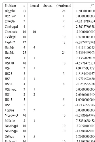
Moreover, we have considered some problems of CUTEr that were used in the recent article by Gratton et al. [21], where the authors compared their new solver BC-DFO with BOBYQA. The detailed list of these problems and their characteristics is provided in Table 1. It shows the name and dimension of the problems, the number of variables which are bounded from below and above and the minimum value f∗which was reported in [21]. If one variable has not an upper or lower bound we used a very large bound for numerical considera-tions (1010or−1010respectively). The results of these experiments can be seen in Table 6.
5.2 Implementation details
We used the default parameters for codes NEWUOA and BOBYQA. We run both codes with a numberm=2n+1 interpolation points using the Frobenius
norm approach, as Powell suggest [38].
Initial points and initial trust-region radius were the same as in the cited references [21, 22, 28, 29, 38].
The stopping criterion that we have used is the same that Powell used, that is, the iterative process stops when the trust-region radius is lower than a tolerance ρend =10−6.
The maximum number of function evaluations allowed for the unconstrained case was:
max f un=9000,for small-size problems, and
max f un=80000,for medium-size problems.
The maximum number of function evaluations allowed for the bound con-strained case was:
max f un=9000,for small-size problems, and
max f un=20000,for medium-size problems.
Problem n lbound ubound (l+u)bound f∗
Biggsb1 25 24 1.50000000000000D-02
Bqp1var 1 1 0.00000000000000D+00
Camel6 2 2 –1.03162845348988D+00
Chebyqad 4 4 2.56057805386809D-22
Chenhark 10 10 –2.00000000000000D+00
Cvxbqp1 10 10 2.47500000000000D+00
Explin2 12 13 –7.09247239439664D+03
Hatflda 4 4 1.61711062151584D-25
Hatfldc 25 24 3.43494690036517D-27
HS1 1 1 7.13660798093435D-24
HS110 10 10 –4.57784755318868D+01
HS2 2 1 4.94122931798918D+00
HS25 3 3 1.81845940377455D-16
HS3 2 1 1.97215226305253D-36
HS38 4 4 2.02675622883580D-28
HS3mod 2 1 0.00000000000000D+00
HS4 2 2 2.66666666400000D+00
HS45 5 5 1.00000000040000D+00
HS5 2 2 –1.91322295498104D+00
Logros 2 2 0.00000000000000D+00
Mccormck 10 10 –9.59800619474625D+00
Mdhole 2 1 7.52316384526264D-35
Ncvxbqp1 10 10 –2.20500000000000D+04
Ncvxbqp2 10 10 –1.43818650000000D+04
Oslbqp 8 5 6.25000000000000D+00
Probpenl 10 10 –2.11912948080046D+05
Pspdoc 4 1 2.41421356237309D+00
Qudlin 12 12 –7.20000000000000D+03
Simbqp 2 1 0.00000000000000D+00
[image:12.612.60.395.75.573.2]Sineali 4 4 –2.83870492243045D+02
Algorithmic parameters in TRB-Powell (Step 1) used: εP =10−6.
η=0.1. We have analyzed other values, but the best results were obtained with
this value ofη.
γ =10−4,σmin=10−10andσmax=1010.
In the conjugate gradient method we have usedεˉ =10−8.
5.3 Numerical results: unconstrained problems
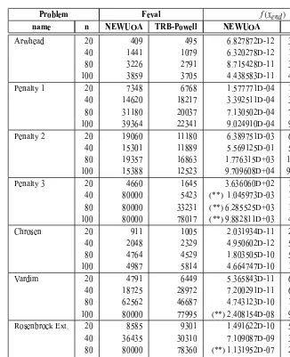
Tables 2 and 3 report the name of the small and medium-size unconstrained optimization problems respectively, the number of function evaluations (Feval) used to reach the stopping criterion and the functional values obtained for TRB-Powell and NEWUOA codes (f(xend)).
The results in Table 2 enable us to make the following observations.
The number of function evaluations required by NEWUOA is the smallest in 16 of the 36 problems while for TRB-Powell this number is the smallest in 17 problems. In the rest of the problems, both algorithms performed the same number of function evaluations.
The average of the evaluations required in this whole set of problems was 1119 for TRB-Powell and 1272 for NEWUOA. In Bard problem NEWUOA got a local minimum while TRB-Powell obtained the global minimum. The obtained functional values are similar for both methods. NEWUOA obtained lower functional values in 18 problems whereas TRB-Powell did it in 14 of them.
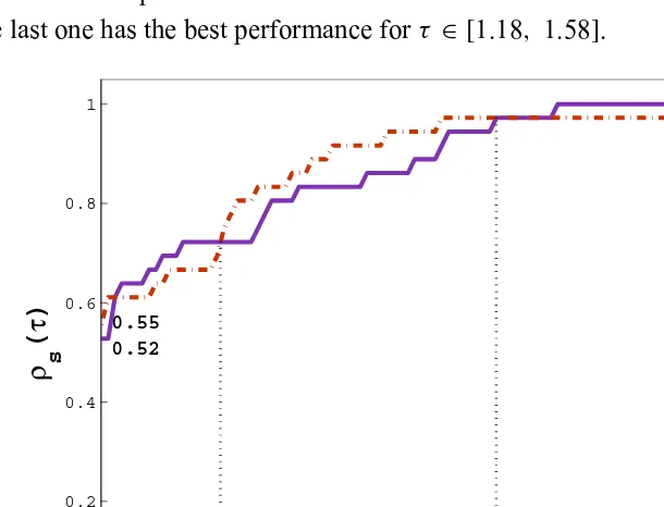
These results are summarized in Figure 1 using the performance profiles described by Dolan and Moré in [16]. Given a set of problems P and a set S of optimization solvers, they compare the performance on problem p∈ Pby a particular algorithm s ∈ S with the best performance by any solver on this problem. Denoting by tp,s the number of function evaluations required when
solving problem p ∈ P by the method s ∈ S, they define the performance
ratio:
rp,s =
tp,s
min{tp,s :s∈ S}
Problem Feval f(xend)
name n NEWUOA TRB-Powell NEWUOA TRB-Powell
Linear Full Rank 9 42 42 3.600000D+01 3.599990D+01 Linear Rank 1 7 159 308 8.380200D+00 8.380202D+00 Linear Rank 1∗ 7 151 225 9.880500D+00 9.880507D+00
Rosenbrock 2 195 134 1.382200D-17 1.089153D-16
Helical valley 3 124 146 2.066500D-13 4.180530D-14 Powell singular 4 476 477 1.099100D-10 1.350267D-10 Freudenstein & Roth 2 76 74 4.898420D+01 4.898420D+01
Bard 3 114 145 1.774900D+00 8.215013D-03
Kowalik & Osborne 4 278 274 3.075000D-04 3.075056D-04
Watson 6 937 1023 2.287600D-03 2.287600D-03
9 9000 9000 (**) 2.160293D-06 (**) 1.782082D-06 12 9000 9000 (**) 5.562963D-07 (**) 4.902148D-08 Box 3-dimensional 3 212 282 3.336000D-17 2.476166D-12 Jennrich & Sampson 2 55 65 1.243621D+02 1.243621D+02 Brown & Dennis 4 191 180 8.582220D+04 8.582220D+04
Chebyqad 6 177 212 4.763800D-13 1.298316D-14
7 229 267 3.148000D-13 2.429278D-14
8 390 247 3.516800D-03 3.516803D-03
9 529 533 2.201700D-13 3.092237D-13
10 666 535 4.772700D-03 4.772713D-03 11 538 657 2.799700D-03 2.799751D-03 Brown almost-linear 10 1255 1153 1.553300D-12 1.588711D-12 Osborne 1 5 1012 1000 6.745600D-05 6.869259D-05 Osborne 2 11 1709 1024 4.013700D-02 4.013741D-02
Bdqrtic 8 432 507 1.023890D+01 1.023897D+01
10 670 522 1.828100D+01 1.828118D+01 11 758 614 2.226000D+01 2.226062D+01 12 781 636 2.627200D+01 2.627277D+01
Cube 5 2842 2050 7.617000D-07 1.277429D-07
6 4625 3080 4.772300D-06 3.328595D-06 8 6825 4580 5.613800D-06 4.744310D-06
Mancino 5 39 55 3.712400D-11 9.547387D-14
8 52 68 1.013600D-08 1.067564D-10
10 68 67 2.292100D-09 1.024540D-08
12 83 89 1.216000D-08 9.571743D-10
Heart 8 8 1118 1001 1.516400D-11 5.108511D-13
[image:14.612.58.398.68.578.2]∗with zero columns and rows
Problem Feval f(xend)
name n NEWUOA TRB-Powell NEWUOA TRB-Powell
Arwhead 20 409 495 6.827872D-12 3.321787D-13
[image:15.612.64.390.66.467.2]40 1441 1079 6.320278D-12 1.322941D-12 80 3226 2791 8.715428D-11 3.022693D-11 100 3859 3705 4.438583D-11 4.041300D-11 Penalty 1 20 7348 6768 1.577771D-04 1.577771D-04 40 14620 18217 3.392511D-04 3.392511D-04 80 31180 20037 7.130502D-04 7.131754D-04 100 39364 22341 9.024910D-04 9.027157D-04 Penalty 2 20 19060 11180 6.389751D-03 6.389759D-03 40 15301 11889 5.569125D-01 5.569250D-01 80 19357 16863 1.776315D+03 1.776315D+03 100 15388 12523 9.709608D+04 9.709608D+04 Penalty 3 20 4660 1645 3.636060D+02 1.008361D-02 40 80000 5423 (**) 1.045973D-03 1.000000D-03 80 80000 33231 (**) 6.285525D+03 1.000000D-03 100 80000 78017 (**) 9.882811D+03 4.658901D-02 Chrosen 20 911 1005 2.031934D-11 2.128075D-13 40 2048 2329 4.950602D-12 5.195116D-12 80 4764 4529 1.803505D-10 5.955498D-11 100 4987 5814 4.664747D-10 1.350874D-10 Vardim 20 4791 6449 5.365843D-11 6.547327D-12 40 18725 28972 7.200291D-11 6.995020D-12 80 62562 46687 4.743123D-10 1.196846D-09 100 80000 77995 (**) 2.408154D-08 9.065575D-08 Rosenbrock Ext. 20 8585 9301 1.491622D-10 5.035342D-12 40 36435 30310 7.109087D-09 3.092178D-12 80 80000 78360 (**) 1.131952D-07 2.712245D-08 100 80000 52891 (**) 2.812546D-07 2.572285D-09 Chebyqad 20 1817 2177 4.572955D-03 4.572955D-03 40 26743 19970 5.960843D-03 5.961027D-03 80 73006 30800 4.931312D-03 4.931938D-03 100 46964 35200 8.715769D-03 4.517172D-03 Table 3 – Medium-size unconstrained problems: NEWUOAvs.TRB-Powell.
They assume thatrp,s ∈ [1,rM] and thatrp,s =rM only when problem p is
not solved by solvers. They also define the fraction
̺s(τ )=
1 np
size{p∈ P :rp,s ≤τ},
In a performance profile plot, the top curve represents the most efficient method within a factorτ of the best measure. The percentage of the test prob-lems for which a given method is best in regard to the performance criterion being studied is given on the left axis of the plot. It is necessary to point out that when both methods coincide with the best result, both receive the corresponding mark. This means that the sum of the successful percentages may exceed 100%. Figure 1 shows the performance profile for both solvers in the interval
[1,1.97]. It can be seen that NEWUOA performs less function evaluations
in 52% of the problems while TRB-Powell does it in 55% of problems and the last one has the best performance forτ ∈ [1.18, 1.58].
1.1 1.3 1.5 1.7 1.9
0 0.2 0.4 0.6 0.8
1 1
0.52 0.55
1.58 1.18
τ
ρ s
(
τ
)
[image:16.612.76.381.233.466.2]NEWUOA TRB-Powell
Figure 1 – Function evaluations in small-size unconstrained problems.
For medium-scale problems we tested eight problems from [38], with dimen-sionn =20,40,80,100. Table 3 reports the numerical results, from which we
can observe:
TRB-Powell required less function evaluations than NEWUOA in 23 of the 32 problems.
NEWUOA was 29611. For eight problems TRB-Powell performed better than NEWUOA (NEWUOA needs more than 10000 extra function evaluations).
In Arwhead, Penalty 3, Rosenbrock Extended, Chrosen (n = 20) and Chrosen (n=80) problems, it can be seen that TRB-Powell was more efficient respect to the final functional value obtained (f(xend)). In particular, the Penalty 3 was
solved significantly better by TRB-Powell than NEWUOA.
TRB-Powell obtained lower functional values than NEWUOA in 18 of 32 problems, while NEWUOA did it in 9. In the rest of the problems both methods achieve the same functional values.
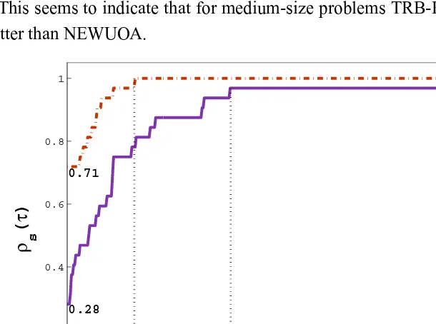
This seems to indicate that for medium-size problems TRB-Powell performs better than NEWUOA.
1 2 3
0 0.2 0.4 0.6 0.8 1
0.28 0.71
0.63 1.51
0.96
τ
ρ s
(
τ
)
NEWUOA TRB-Powell
[image:17.612.74.379.241.468.2]1
Figure 2 – Function evaluations in medium-size unconstrained problems.
These results are summarized in Figure 2 using the performance profiles described before. Since rp,s is large for several medium-size problems, we
used a logarithmic scale in base 2 in thex-axis, as recommended in [16]. Thus, we draw
̺s(τ )=
1 np
Problem Feval f(xend)
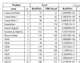
name n BOBYQA TRB-Powell BOBYQA TRB-Powell
Linear Full Rank 9 31 31 1.699999D+02 1.699999D+02 Linear Rank 1 7 84 82 8.380281D+00 8.380281D+00 Linear Rank 1∗ 7 90 82 9.880597D+00 9.880597D+00
Rosenbrock 2 171 170 4.720012D-12 4.213517D-09 Powell singular 4 131 83 4.840000D-04 4.840000D-04 Kowalik & Osborne 4 162 90 4.470176D-04 4.470176D-04 Brown Dennis 4 170 168 8.582220D+04 8.582220D+04
HS45 5 44 43 1.000000D+00 1.000000D+00
HS46 5 49 38 4.930380D-32 4.930380D-32
HS56 7 119 98 1.052166D-12 2.148472D-12
HS77 5 140 108 2.130995D-11 2.424337D-11
HS79 5 128 133 8.368490D-13 1.026634D-12
HS107 9 195 158 5.909464D-13 3.809796D-13
HS110 10 206 172 -4.577847D+01 -4.577847D+01
Rastrigin 10 69 68 2.487372D+02 2.487372D+02
Schwefel 10 90 73 -4.189829D+03 -4.189829D+03
[image:18.612.65.387.63.315.2]∗with zero columns and rows
Table 4 – Small-size bounded constrained problems: BOBYQAvs.TRB-Powell.
whererM >0 is such thatrp,s ≤rM, for all pands.
Figure 2 shows that TRB-Powell solved this set of problems successfully. TRB-Powell had a better performance in 71% of the problems.
5.4 Numerical results: bound constrained problems
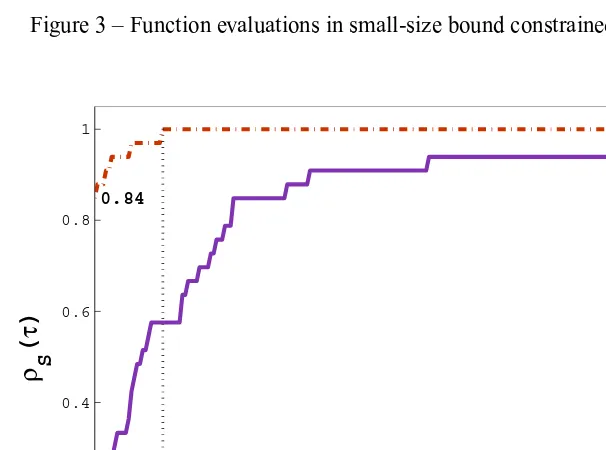
Tables 4 and 5 show the performance of BOBYQA and TRB-Powell for small and medium-size bound constrained problems, respectively. We observe in Ta-ble 4 that the number of function evaluations required by TRB-Powell is less than BOBYQA in 14 of the 16 test problems. Moreover, the obtained func-tional values were similar for both methods. This performance of TRB-Powell has been depicted in Figure 3, where it has required less function evaluations in 93% of the problems.
Problem Feval f(xend)
name n BOBYQA TRB-Powell BOBYQA TRB-Powell
Invdist2 20 182 236 3.220305D+01 3.220305D+01
40 943 826 1.677709D+02 1.677709D+02
60 6990 4832 4.081079D+02 4.087195D+02 80 5158 6125 7.699010D+02 7.689744D+02 100 20000 20000 (**) 1.251662D+03 (**) 1.248745D+03
Arwhead 20 636 558 1.826050D-11 4.961897D-11
40 1458 1468 1.208688D-09 1.054593D-08 80 3677 4332 8.622840D-10 1.097986D-09 100 6605 2927 3.969482D-08 2.774640D-09
Chrosen 20 242 235 1.900000D+01 1.900000D+01
40 464 612 3.900000D+01 3.900000D+01
80 864 825 7.900000D+01 7.900000D+01
100 1055 1037 9.900000D+01 9.900000D+01 Penalty 1 20 5677 5253 1.577706D-04 1.577901D-04 40 15006 11645 3.392511D-04 3.392517D-04 80 19410 15680 7.130502D-04 7.130518D-04 100 20000 17458 (**) 9.024911D-04 9.024942D-04 Chebyqad 20 2245 2020 4.572955D-03 4.572956D-03 40 20000 19617 (**) 5.960849D-03 5.960854D-03 80 20000 20000 (**) 4.932619D-03 (**) 4.933963D-03 100 20000 20000 (**) 4.523622D-03 (**) 4.566568D-03 Rastrigin 20 120 114 4.974745D+02 4.974745D+02 40 1301 297 9.949489D+02 9.949489D+02
80 600 613 1.989898D+03 1.989898D+03
100 820 795 2.487372D+03 2.487372D+03
Griewangk 20 882 523 6.312884D-11 3.234968D-12 40 2091 1309 7.525736D-11 1.494938D-11 80 12436 3031 2.297593D-10 1.809503D-10 100 5213 3927 2.405037D-10 6.107597D-10
Ackley 20 570 526 9.132573D-06 9.355251D-07
[image:19.612.69.389.67.480.2]40 1129 1231 9.987129D-07 1.001365D-06 80 2112 1923 9.156053D-06 9.086830D-06 100 2968 2406 8.297680D-07 9.516777D-06 Table 5 – Medium-size bounded constrained problems: BOBYQAvs.TRB-Powell.
1 1.1 1.2 1.3 1.4 1.5 1.6 1.7 1.8 1.9 0
0.1 0.2 0.3 0.4 0.5 0.6 0.7 0.8 0.9 1
0.12 0.93
τ
ρ S
(
τ
)
BOBYQA TRB-Powell
1.02
[image:20.612.80.377.73.301.2]1
Figure 3 – Function evaluations in small-size bound constrained problems.
0 0.2 0.4 0.6 0.8 1 1.2 1.4 1.6 1.8 2
0 0.2 0.4 0.6 0.8 1
0.24 0.84
τ
ρ S
(
τ
)
BOBYQA TRB-Powell
1
0.24
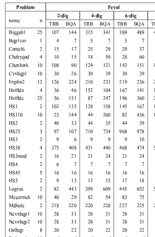
[image:20.612.75.378.346.571.2]Problem Feval
2-dig 4-dig 6-dig 8-dig
name n
TRB BQA TRB BQA TRB BQA TRB BQA
Biggsb1 25 107 144 315 341 389 489 464 548
Bqp1var 1 4 7 5 7 5 7 5 7
Camel6 2 15 17 25 29 29 37 31 41
Chebyqad 4 10 15 18 50 28 60 48 64
Chenhark 10 108 90 124 121 143 151 161 172
Cvxbqp1 10 30 26 30 39 30 39 30 39
Explin2 12 126 224 210 233 219 236 227 258
Hatflda 4 36 46 152 104 167 141 180 182
Hatfldc 25 56 131 87 247 196 360 276 441
HS1 2 102 135 128 158 145 167 158 172
HS110 10 23 144 44 260 82 436 188 521
HS2 2 40 33 44 35 44 39 44 39
HS25 3 97 107 710 734 968 978 f 995
HS3 2 9 6 9 9 9 10 9 10
HS38 4 375 408 431 440 468 474 501 503
HS3mod 2 16 21 21 24 21 24 21 24
HS4 2 6 7 7 7 7 7 7 7
HS45 5 16 16 16 16 16 16 16 16
HS5 2 9 13 12 15 17 18 22 21
Logros 2 82 443 399 609 445 652 547 661
Mccormck 10 40 29 82 54 83 75 99 87
Mdhole 2 218 220 220 220 227 225 228 225
Ncvxbqp1 10 28 31 28 31 28 31 28 31
Ncvxbqp2 10 28 31 28 31 28 31 28 31
Oslbqp 8 20 22 20 22 20 22 20 22
Probpenl 10 f f f f f f f f
Pspdoc 4 40 41 50 55 57 57 65 65
Qudlin 12 32 34 32 34 32 34 32 34
Simbqp 2 12 12 12 12 12 12 12 12
[image:21.612.70.386.80.563.2]Sineali 4 12 36 17 260 17 387 17 432
Table 6 shows the results obtained by BOBYQA (BQA) and TRB-Powell (TRB) on the experiments with the problems described in Table 1. It shows the name of the problem, the number of function evaluations needed by TRB-Powell and BOBYQA to attain two, four, six and eight significant figures of the objective function value f∗, reported by the authors of [21]. We indicate with “f” when a problem do not obtain the precision required.
The results reported in Table 6 show that both solvers fail to solve one test problem in all four cases. Moreover, TRB-Powell did not obtain the precision of 8 digits in the HS25 problem. For low accuracy BOBYQA solved 17% of the test cases faster than TRB-Powell and TRB-Powell solved 73% of the problems faster. For 8 correct significant figures, BOBYQA solved 17% of the test cases faster, and TRB-Powell 67% of the problems faster. For 4 and 6 significant digits BOBYQA solved 13% of the test cases faster than TRB-Powell and TRB-Powell solved 67% and 70% of the problems faster, respectively.
6 Conclusions
We have presented a modified version of the algorithms NEWUOA and BOBYQA for solve unconstrained and bound constrained derivative-free optimization problems. Our method use an active-set strategy for solving the trust-region subproblems. Since we consider the infinity norm, a box constrained quadratic optimization problem has to be solved at each iteration.
We have compared our new version TRB-Powell with the original NEWUOA and BOBYQA. The numerical results reported in this paper are encouraging and suggest that our algorithm takes advantage of the active-set strategy to explore the trust-region box. The number of function evaluations was reduced in most of the cases. These promising numerical results and the new articles by M.J.D. Powell [39, 40] encourage us for further development in constrained optimiza-tion without derivatives.
REFERENCES
[1] P. Alberto, F. Nogueira, H. Rocha and L. Vicente, Pattern search methods for user-provided points: Application to molecular geometry problems. SIAM Journal on Optimization,14(4) (2004), 1216–1236.
[2] R. Andreani, E. Birgin, J.M. Martínez and M.L. Schuverdt, On augmented la-grangian methods with general lower-level constraints. SIAM Journal on Opti-mization,18(2007), 1286–1309.
[3] R. Andreani, E. Birgin and J.M. Martínez and M.L. Schuverdt, Augmented la-grangian methods under the constant positive linear dependence constraint qual-ification. Mathematical Programming,111(2008), 5–32.
[4] C. Audet and J. Dennis Jr., A pattern search filter method for nonlinear program-ming without derivatives. SIAM Journal on Optimization,14(4) (2004), 980–1010. [5] F. Berghen and H. Bersini, CONDOR: a new parallel, constrained extension of Powell’s UOBYQA algorithm: Experimental results and comparison with the DFO algorithm. Journal of Computational and Applied Mathematics, 181(1) (2005), 157–175.
[6] E. Birgin, R. Castillo and J.M. Martínez, Numerical comparison of augmented lagrangian algorithms for nonconvex problems.Computational Optimization and Applications,31(2005), 31–56.
[7] E. Birgin and J.M. Martínez, Large-scale active-set box-constrained optimiza-tion method with spectral projected gradients.Computational Optimization and Applications,23(1) (2002), 101–125.
[8] E. Birgin and J.M. Martínez, Improving ultimate convergence of an augmented lagrangian method.Optimization Methods and Software,23(2008), 177–195. [9] E. Birgin, J.M. Martínez and M. Raydan, Nonmonotone spectral projected
gradi-ent methods on convex sets.SIAM Journal on Optimization,10(2000).
[10] A. Booker, J. Dennis Jr., P. Frank, D. Serafini and V. Torczon, Optimization using surrogate objectives on a helicopter test example. Computational Methods for Optimal Design and Control, J. Borggaard, J. Burns, E. Cliff and S. Schreck eds. Birkhäuser, (1998), 49–58.
[12] A. Conn, K. Scheinberg and P. Toint,Recent progress in unconstrained nonlinear optimization without derivatives. Mathematical Programming, 79(1997), 397– 414.
[13] A. Conn, K. Scheinberg and P. Toint, A derivative free optimization algorithm in practice.In Proceedings of the 7th AIAA/USAF/NASA/ISSMO Symposium on Multidisciplinary Analysis and Optimization, St. Louis, MO (1998).
[14] A. Conn, K. Scheinberg and L. Vicente,Introduction to derivative-free optimiza-tion.SIAM (2009).
[15] J.E. Dennis and V. Torczon, Direct search methods on parallel machines.SIAM Journal on Optimization,1(1991), 448–474.
[16] E. Dolan and J. Moré, Benchmarking optimization software with performance profiles.Mathematical Programming,91(2002), 201–213.
[17] R. Duvigneau and M. Visonneau, Hydrodynamic design using a derivative-free method.Structural and Multidisciplinary Optimization,28(2) (2004), 195–205. [18] G. Fasano, J. Morales and J. Nocedal, On the geometry phase in model-based
algorithms for derivative-free optimization. Optimization Methods and Software, 24(1) (2009), 145–154.
[19] K. Fowler, J. Reese, C. Kees, J. Dennis Jr., C. Kelley, C. Miller, C. Audet, A. Booker, G. Couture, R. Darwin, M. Farthing, D. Finkel, J. Gablonsky, G. Gray and T. Kolda, A comparison of derivative-free optimization methods for groundwater supply and hydraulic capture community problems.Advances in Water Resources, 31(5) (2008), 743–757.
[20] N.I. Gould, D. Orban and Ph.L. Toint, CUTEr and SifDec: A constrained and unconstrained testing environment, revisited.ACM Transactions on Mathematical Software,29(4) (2003), 373–394.
[21] S. Gratton, Ph.L. Toint and A. Tröltzsch, An active-set trust region method for derivative-free nonlinear bound-constrained optimization.Technical Report. CERFACS. Parallel Algorithms Team.,10(2010), 1–30.
[22] W. Hock and K. Schittkowski, Nonlinear programming codes, Lecture Notes in Economics and Mathematical Systems, Springer,187(1980).
[24] T. Levina, Y. Levin, J. McGill and M. Nediak, Dynamic pricing with online learning and strategic consumers: An application of the aggregation algorithm. Operations Research (2009), 385–482.
[25] M. Marazzi and J. Nocedal, Wedge trust region methods for derivative free opti-mization.Mathematical Programming,91(2) (2002), 289–305.
[26] A. Marsden, M. Wang, J. Dennis and P. Moin, Optimal aeroacustic shape de-sign using the surrogate management framework.Optimization and Engineering, 5(2) (2004), 235–262.
[27] J. Meza and M.L. Martínez,On the use of direct search methods for the molecular conformation problem.J. Comput. Chem.,15(6) (1994), 627–632.
[28] M. Molga and C. Smutnicki, Test functions for optimization needs.Available at http://www.zsd.ict.pwr.wroc.pl/files/docs/functions.pdf (2005).
[29] J. Moré and S. Wild, Benchmarking derivative-free optimization algorithms. SIAM Journal on Optimization,20(1) (2009), 172–191.
[30] P. Mugunthan, C. Shoemaker and R. Regis, Comparison of function approxima-tion, heuristic and derivative-based methods for automatic calibration fo com-putationally expensive groundwater bioremediation models.Water Resour. Res., 41(11) (2005), 1–17.
[31] J. Nelder and R. Mead, A simplex method for function minimization.Computer Journal,7(1965), 308–313.
[32] R. Oeuvray, Trust-region methods based on radial basis functions with applica-tion to biomedical imaging.Ph.D. thesis (2005).
[33] R. Oeuvray and M. Bierlaire, A new derivative-free algorithm for the medical image registration problem.International Journal of Modelling and Simulation, 27(2) (2007), 115–124.
[34] M.J.D. Powell, On the Lagrange functions of quadratic models that are defined by interpolation.Optimization Methods and Software,16(2001), 289–309. [35] M.J.D. Powell, UOBYQA: Unconstrained optimization by quadratic
approxima-tion.Mathematical Programming,92(3) (2002), 555–582.
[36] M.J.D. Powell, On trust region methods for unconstrained minimization without derivatives.Mathematical Programming,97(3) (2003), 605–623.
[38] M.J.D. Powell, The NEWUOA software for unconstrained optimization with-out derivatives. Nonconvex Optimization and Its Applications, Springer US, 83(2006).
[39] M.J.D. Powell,Developments of NEWUOA for minimization without derivatives. IMA Journal of Numerical Analysis,28(4) (2008), 649–664.
[40] M.J.D. Powell, The BOBYQA algorithm for bound constrained optimization without derivatives. Technical report, Department of Applied Mathematics and Theoretical Physics, Cambridge University, Cambridge, England (2009). [41] V. Torczon, On the convergence of pattern search algorithms.SIAM Journal on
Optimization,7(1) (1997), 1–25.
[42] D. Winfield, Functions and functional optimization by interpolation in data tables.Ph.D. thesis (1969).