A GRASP algorithm to solve the problem of dependent tasks scheduling in different machines

A GRASP algorithm to solve the problem of

dependent tasks scheduling in different

machines

Manuel Tupia Anticona Pontificia Universidad Católica del Perú

Facultad de Ciencias e Ingeniería, Departamento de Ingeniería, Sección Ingeniería Informática

Av. Universitaria cuadra 18 S/N Lima, Perú, Lima 32 tupia.mf@pucp.edu.pe

Abstract. Industrial planning has experienced notable advancements since its beginning by the middle of the 20th century. The importance of its application within the several industries where it is used has been demonstrated, regardless of the difficulty of the design of the exact algorithms that solve the variants. Heuristic methods have been applied for planning problems due to their high complexity; especially Artificial Intelligence when developing new strategies to solve one of the most important variants called task scheduling. It is possible to define task scheduling as: .a set of N production line tasks and M machines, which can execute those tasks, where the goal is to find an execution order that minimizes the accumulated execution time, known as makespan. This paper presents a GRASP meta heuristic strategy for the problem of scheduling dependent tasks in different machines

1 Introduction

The task-scheduling problem has its background in industrial planning [1] and in task-scheduling in the processors of the beginning of microelectronics [2]. That kind of problem can be defined, from the point of view of combinatory optimization [3], as follows:

fulfilling certain conditions that satisfy the optimality of the required solution for the problem.

The scheduling problem presents a series of variants depending on the nature and the behavior of both, tasks and machines. One of the most difficult to present variants, due to its high computational complexity is that in which the tasks are dependent and the machines are different.

In this variant each task has a list of predecessors and to be executed it must wait until such is completely processed. We must add to this situation the characteristic of heterogeneity of the machines: each task lasts different execution times in each machine. The objective will be to minimize the accumulated execution time of the machines, known as makespan [3]

Observing the state of the art of the problem we see that both its practical direct application on industry and its academic importance, being a NP-difficult problem, justifies the design of a heuristic algorithm that search for an optimal solution for the problem, since there are no exact methods to solve the problem. In many industries such as assembling, bottling, manufacture, etc., we see production lines where wait periods by task of the machines involved and saving the resource time are very important topics and require convenient planning.

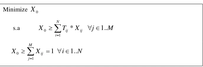
From the previous definition we can present a mathematical model for the problem as in the following illustration and where it is true that:

• X0 represents makespan

• Xij will be 0 if the j-esim machine does not execute the i-esim task and 1 on the

contrary.

Minimize

X

s.a

∑

=

≥

i

ij ij

X

T

X

1

0

*

∀

j

∈

1

..

M

1

1

0

≥

∑

=

= M

j ij

X

X

∀

i

∈

1

..

N

Fig. 1. A mathematical model for the task-scheduling problem.

1.1 Existing methods to solve the task-scheduling problem and its variants

The existing solutions that pretend to solve the problem, can be divided in two groups: exact methods and approximate methods.

exploration). Nevertheless, a search and scheduling strategy that analyzes every possible combination is computationally expensive and it only works for some kinds (sizes) of instances.

Approximate methods [3, 4 and 5] on the other hand, do try to solve the most complex variants in which task and machine behavior intervenes as we previously mentioned. These methods do not analyze exhaustively every possible pattern combinations of the problem, but rather choose those that fulfill certain criteria. In the end, we obtain sufficiently good solutions for the instances to be solved, what justifies its use.

1.2 Heuristic Methods to Solve the Task-scheduling variant

According to the nature of the machines and tasks, the following subdivision previously presented may be done:

• Identical machines and independent tasks

• Identical machines and dependent tasks

• Different machines and independent tasks

• Different machines and dependent tasks: the most complex model to be studied in this document.

Some of the algorithms proposed are:

A Greedy algorithm for identical machines propose by Campello and Maculan [3]: the proposal of the authors is to define the problem as a discreet programming one (what is possible since it is of the NP-difficult class), as we saw before.

Using also, Greedy algorithms for different machines and independent tasks, like in the case of Tupia [10] The author presents the case of the different machines and independent tasks. Campello and Maculan’s model was adapted, taking into consideration that there were different execution times for each machine: this is, the matrix concept that it is the time that the i-esim task takes to be executed by the j-esim machine appears.

A GRASP algorithm, as Tupia [11]. The author presents here, the case of the different machines and independent tasks. In this job the author extended the Greedy criteria of the previous algorithm applying the conventional phases of GRASP technique and improving in about 10% the results of the Greedy algorithm for instances of up to 12500 variables (250 tasks for 50 machines).

1.3 GRASP Algorithms

such a way that, instead of selecting a sole element, it forms a group of elements, that candidate to be part of the solution group and fulfill certain conditions, it is about this group that a random selection of some of its elements.

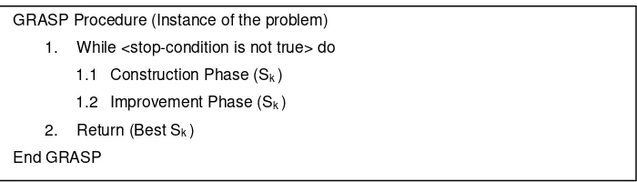
This is the general scheme for GRASP technique:

GRASP Procedure (Instance of the problem)

1. While <stop-condition is not true> do

1.1 Construction Phase (Sk )

1.2 Improvement Phase (Sk )

2. Return (Best Sk )

End GRASP

Fig. 2. General structure of GRASP algorithm

About this algorithm we can affirm:

Line 1: the GRASP procedure will continue while the stop condition is not fulfilled. The stop condition can be of several kinds: optimality (the result obtained presents a certain degree of approximation to the exact solution or it is optimal enough); number of executions carried out (number of interactions); processing time (the algorithm will be executed during a determined period of time).

Lines 1.1 and 1.2: the two main phases of a GRASP algorithm are executed, later: construction stage of the adapted random Greedy solution; and the stage of improvement of the previously constructed solution (combinatorial analyses of most cases).

2 Proposed GRASP Algorithm

We must start from the presumption that there is a complete job instance that includes what follows: a quantity of task and machines (N and M respectively); an execution time matrix T and the lists of predecessors for each task in case there were any.

2.1 Data structures used by the algorithm

Let us think that there is at least one task with predecessors that will become the initial one within the batch, as well as there are no circular references among predecessor tasks that impede their correct execution:

Processing Time Matrix T: (Tij) MxN, where each entry represents the time it takes

Accumulated Processing Times Vector A: (Ai), where each entry Ai is the

accumulated working time of Mi machine.

Pk: Set of predecessor tasks of Jk task.

Vector U: (Uk) with the finalization time of each Jk task.

Vector V: (Vk) with the finalization time of each predecessor task of Jk, where it is true

that Vk =

=

max{

U

},

J

∈

P

Si: Set of tasks assigned to Mi machine.

E: Set of scheduled tasks

C: Set of candidate tasks to be scheduled

Fig. 3. Data structures used by the algorithm

We are going to propose to selection criteria during the development of the GRASP algorithm, what is going to lead us to generate two relaxation constants instead of only one:

• Random GRASP selection criteria for the best task to be programmed, using relaxation constant α.

• Random selection criteria for the best machine that will execute the task selected before, using an additional θ parameter.

2.2 Selection criteria for the best task

These criteria bases on the same principles as the Greedy algorithm presented before:

Identifying the tasks able to be programmed: this is, those that have not been programmed yet and its predecessors that have already been executed (or do not present predecessors).

For each one of the tasks able, we have to generate the same list as in the Greedy algorithm: accumulated execution times shall be established starting from the end of the last predecessor task executed.

The smallest element from each list must be found and stored in another list of local minimums. We shall select the maximum and minimum values of the variables out of this new list of local minimums: worst and best respectively.

We will form a list of candidate tasks RCL analyzing each entry of the list of local minimums: if the corresponding entry is within the interval [best, best+

2. 3 Selection criteria for the best machine

Once a task has been selected out of RCL, we look for the best machine that can execute it. This is the main novelty of the algorithm proposed. The steps to be followed are the next ones:

The accumulated time vector is formed once again from the operation of the predecessors of the j-esim task, which is being object of analyses. Maximum and minimum values of the variables are established: worst and best respectively.

Then we form the list of candidate machines MCL: each machine that executes the j-esim task in a time that is in the interval (best, best+ θ*(worst-best)) is part of the MCL. Likewise, we will select one of them by chance, which will be the executioner of the j-esim task.

2. 4 Presentation of the algorithm

GRASP Algorithm_Construction (M, N, T, A, S, U, V, α, θ) 1. Read and initialize N, M, α, θ, J1, J2,…,JN, T, A, S, U, V

2. E = ø

3. While |E| ≠ N do 3.1 C = ø

3.2 best = +

∞

If (Pℓ ⊆ E) ^ (Jℓ∈E) => C = C ∪ {Jℓ}

3.5 Bmin = ø

3.6 For each Jℓ∈ C do

3.6.1 VL

max

{

U

}

=

3.6.2 Bmin = Bmin

∪

Min

{

T

+

max{

A

,

V

}}

3.7 best = Min {Bmin} {Selection of the best task. Formation of RCL} 3.8 worst = Max {Bmin}

3.9 RCL = ø

3.10 For each Jℓ∈ C do

If

Min

{

T

+

max{

A

,

V

}}

RCL = RCL ∪ {Jℓ}

3.11 k = ArgRandomJLeRCL{RCL}

3.12 MCL = ø {Selection of the best machine} 3.13 best =

Min

{

T

+

max{

A

,

V

}}

Max

{

T

+

max{

A

,

V

}}

If

T

+

max{

A

,

V

}

{Mi}

3.16 i =

ArgAleator

io

{

MCL

}

3.17

S

S

∪

{

J

}

∪

{

J

}

3.19Ai =

T

+

max{

A

,

V

}

3.20 Uk = Ai

End While 3

4. makespan =

max

A

S

∀

i

∈

[

1

,

M

]

End GRASP Algorithm_construction

Comments on the GRASP Algorithm proposed:

• Line 1: entry of the variables e initialization of the data structures needed for the working instance as N, M, T, A, U, V, E, Si for each machine, α, θ etc.

• Line 2: the process ends when all the programmed tasks of the batch are in group E.

• Line 3.1: the list of apt tasks C is initialized empty.

• Line 3.2: best and worst variables that will be used to work the intervals of the relaxation criteria are initialized.

• Line 3.4: the list of apt tasks C is formed

• Line 3.5: the list of local minimums Bmin is initialized.

• Line 3.6 – 3.6.2: entries corresponding to list V are actualized; list Bmin is formed adding each minor element of the accumulated time list of each task.

• Lines 3.7 – 3.8: maximum and minimum values of Bmin are assigned to worst and best variables respectively.

• Line 3.9: RCL list is initialized empty

• Lines 3.10 – 3.11: RCL list is formed when the condition }}

, max{ {

] , 1

[ M pl p l

p T A V

Min _∈ + ∈ [best, best + α* (worst-best)] is true, then an element from this list (k) is chosen by chance.

• Lines 3.12 – 3.16: minimum and maximum execution times for the task selected in 3.11 are chosen. MCL will form from the machines that execute such task fulfilling the condition: Tik +max{Ai,Vk}∈ [best, best + θ* (worst-best)]. In the end a machine is also chosen in an aleatoric way (variable i).

• Lines 3.17 – 3.20: structures E, A, U and Si are actualized where it

corresponds.

• Line 3: makespan is determined as the major entry of A.

3. Numeric Experiences

The instances with which the algorithm was tested are formed by an M quantity of machines, N of task and a T matrix of execution times. The values used for M and N, respectively, were:

• Number of tasks N: within the interval of 100 to 250, taking 100, 150, 200 and 250 values as points of reference.

• Number of machines M: a maximum of 50 machines taking 12, 25, 37 and 50 values as point of reference.

• Processing time matrix: it will be generated in a random way with values from 1 to 100 time units1_.

We have a total of 16 combinations for the machine-tasks combinations. Likewise, for each combination 10 different instances will be generated, which gives a total of 160 test problems solved.

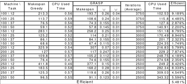
3.1 Quality of the GRASP solution compared to a simply Greedy solution

As there is no literature on pre-determined test instances for such problem, we decided to confront the results with those of a Greedy algorithm2_{. In the first}

summary table average results of Greedy and GRASP algorithms execution (in that order) over the respective instances are shown; CPU times consumed by both algorithms, the quantity of executed iterations in the GRASP Construction phase and the values assigned to constants α and θ; finally the efficiency of the GRASP result over the Greedy result calculated as follows is also shown: 1-(GRASP Result/Greedy Result)

Table 1. Summary table of GRASP vs. Greedy numeric experiments

1

: We shall notice that a very high execution time (+ oo) may be interpreted as if the machine does not execute a determined task. In this case an execution time equal to 0 may be confuse as the machine executes the task so fast that it does it instantaneously, without taking time

2

: In order to have a Greedy behavior it is enough to make constant a equal to 0 without regardless of selection of the best machine; that is why the algorithm is not added.

E ffici en t M a k e sp a n ∪ ∪

1 0 0 \ 1 2 2 1 3 .3 0 .5 6 1 9 3 .7 0 .26 0.0 4 3 75 0 1 0 2.5 3 9 .1 8 9 % 1 0 0 \ 2 5 1 1 3 .7 0 .5 9 1 0 8 .6 0 .24 0.0 1 3 75 0 1 15 .8 4 .4 8 5 % 1 0 0 \ 3 7 7 6 .5 0 .5 6 7 4 .3 0.1 55 0.0 1 3 75 0 1 27 .6 2 .8 7 6 % 1 0 0 \ 5 0 5 9 .1 0 .5 2 5 7 .8 0.1 45 0.0 1 3 75 0 1 4 0.9 1 2 .2 0 0 % 1 5 0 \ 1 2 2 8 3 .1 0 .5 8 2 5 8 .2 0 .25 0.0 1 3 00 0 1 5 1.1 8 8 .7 9 5 % 1 5 0 \ 2 5 1 2 5 .2 0 .5 2 1 14 0 .21 0.0 1 3 00 0 1 7 0.4 9 8 .9 4 6 % 1 5 0 \ 3 7 8 6 .1 0 .5 5 8 4 .1 0.1 55 0.0 1 3 00 0 2 01 .7 2 .3 2 3 % 1 5 0 \ 5 0 6 8 .6 0 .5 3 6 7 .4 0.1 15 0.0 1 3 00 0 2 2 4.3 5 1 .7 4 9 % 2 0 0 \ 1 2 3 2 5 .9 0 .5 4 3 07 0 .07 0.0 1 2 50 0 2 1 6.8 3 5 .7 9 9 % 2 0 0 \ 2 5 1 27 0 .5 7 1 17 0.2 47 0.0 1 2 50 0 2 29 .2 7 .8 7 4 % 2 0 0 \ 3 7 1 0 9 .8 0 .5 7 1 0 5 .2 0.1 12 0.0 1 2 50 0 2 4 8.7 5 4 .1 8 9 % 2 0 0 \ 5 0 7 6 .4 0 .4 7 7 4 .6 0.1 55 0.0 1 2 50 0 2 7 4.5 8 2 .3 5 6 % 2 5 0 \ 1 2 4 1 1 .8 0 .4 6 3 7 7 .1 0 .15 0.0 1 2 50 0 2 49 .2 8 .4 2 6 % 2 5 0 \ 2 5 1 8 3 .5 0 .5 8 1 6 8 .2 0 .28 0.0 1 2 50 0 2 8 2.3 4 8 .3 3 8 % 2 5 0 \ 3 7 1 2 5 .3 0 .5 7 1 1 9 .6 0 .26 0.0 1 2 50 0 3 0 9.0 3 4 .5 4 9 % 2 5 0 \ 5 0 9 6 .5 0 .5 5 9 1 .1 0.1 23 0.0 1 2 50 0 3 4 3.3 2 5 .5 9 6 % 5 .4 8 1 % C P U U s e d

T im e Ite r atio n s (A v e ra g e )

E fficien t M a ch in e \

T a s k

M a k e sp a n G re e d y

C P U U s e d T im e

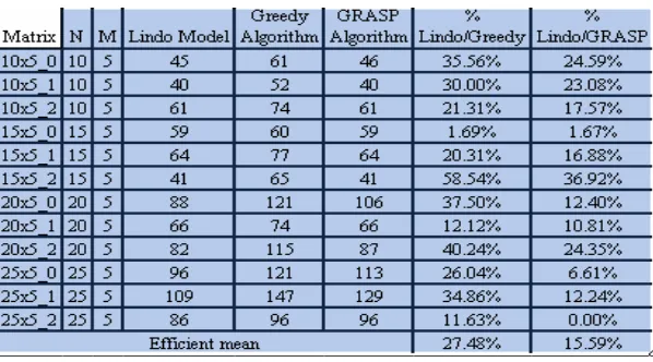
3.2 Real quality of the GRASP solution confronted with mathematical model‘s

solutions

In order to determine the real quality of the solutions we decided to apply the mathematical model of the problem to linear programming problem solver packages as LINDO tool in its student version, in order to obtain exact solutions and confront them with those of the proposed GRASP algorithm.

The two tables that follow summarize the exact results obtained confronted with the heuristic (voracious solution) and meta heuristic (GRASP solution) results. In addition to this we will present the values of the relaxation constants used for the GRASP construction phase where nearly 7000 iterations for all the cases were carried out.

Table 2. Experimental results for M = 3

4. Conclusions

Both criteria adapted to the kind of algorithm presented: the criteria were voracious in the case of the voracious algorithm (un-modifiable selection); or adaptable and random as in the case of the GRASP algorithm. In the literature there are not any GRASP algorithm that considers a double relaxation criteria at the moment of making the correspondent selections: conventional GRASP ones, were just part of a RCL list of candidates for the tasks to be executed. In 100% of the cases the result of the GRASP algorithm is better than that of voracious algorithm for high enough test instances (proportion 4 to 1, 5 to 1). In small instances it is at least equal to the voracious solution or it does not reach the same level by a very little percentage. The percentage of advantage of the GRASP algorithm confronted to the voracious algorithm is in average 5%.

GRASP algorithm get much closer to the exact solution for analyzed instances, within an average range of 5% to 9% of those solutions. In multiple cases it equals the solution, behavior that has been seen as we reduce the task-machine proportions, this is, when the number of available machine increases.

REFERENCES

[1] G. Miller, E. Galanter. Plans and the Structure of Behavior. Holt Editorial, 1960. [2] M. Drozdowski. Scheduling multiprocessor tasks: An overview. European Journal Operation Research, 1996, pp. 215 - 230.

[3] R. Campello, N. Maculan. Algorithms e Heurísticas: desenvolvimiento e avaliaçao de performance. Apolo Nacional Editores. Brasil, 1992.

[4] M. Pinedo. Scheduling: Theory, Algorithms and Systems, Prentice Hall, 2002. [5] T. Feo, M. Resende, Greedy Randomized Adaptive Search Procedure. In Journal of Global Optimization, No. 6, 1995, pp. 109-133.

[6] W. Rauch, Aplicaciones de la inteligencia Artificial en la actividad empresarial, la ciencia y la industria - tomo II. Editorial Díaz de Santos. España, 1989.

[7] P. Kumara Artificial Intelligence: Manufacturing theory and practice. NorthCross - Institute of Industrial Engineers, 1988.

[8] A. Blum, M. Furst. Fast Planning through Plan-graph Analysis. In 14th International Joint Conference on Artificial Intelligence. Morgan- Kaufmann Editions, 1995, pp. 1636 -1642.

[9] R. Conway. Theory of Scheduling, Addison–Wesley Publishing Company, 1967 [10] M. Tupia. Algoritmo voraz para resolver el problema de la programación de tareas dependientes en máquinas diferentes. In International Conference of Industrial Logistics (7, 2005, Uruguay) ICIIL. Editors. H. Cancela, Montevideo – Uruguay, 2005, p. 345.