Immune algorithm for solving the smooth economic dispatch problem

Immune Algorithm for Solving the Smooth

Economic Dispatch Problem

Victoria S. Arag´on and Susana C. Esquivel

Laboratorio de Investigaci´on y Desarrollo en Inteligencia Computacional (LIDIC) Universidad Nacional de San Luis

Ej´ercito de los Andes 950 - (5700) San Luis, ARGENTINA CONICET

Abstract. In this paper, an algorithm inspired on the T-Cell model

of the immune system is presented, it is used to solve Economic Dis-patch Problems with smooth objective function. The proposed approach is called IA EDP S, which stands forImmune Algorithm for Economic Dispatch Problem for smooth objective function, and it uses as differenti-ation process a redistribution power operator. The proposed approach is validated using five problems taken from the specialized literature. Our results are compared with respect to those obtained by several other approaches.

Keywords:Artificial immune systems , economic dispatch problem ,

meta-heuristics

1

Introduction

The objective of Economic Dispatch Problem (EDP) is to minimize the total generation cost of a power system while satisfying several constraints associated to the system, such as load demands, ramp rate limits, maximum and minimum limits, and prohibited operating zones. The objective function type (smooth or non smooth) and the constraints which are considered in the problem will determine how hard is to solve the problem.

Over the last years, several methods have been proposed to solve the EDP. They can be divided in three main groups: classical, based on artificial intelli-gence (AI) and hybrid methods. Classical methods have been proposed to solve EDP, but they suffer from some limitations (for instance, the objective functions and the constraints must be differentiable). On the other hand, modern heuristic algorithms have proved to be able to deal with nonlinear optimization problems, e.g., EDPs. Surveys about these techniques can be found in [14] and [2].

The remainder of this paper is organized as follows. Section 2 defines the economic dispatch problem. In Section 3, we describe our proposed algorithm. In Section 4, we present the test problems used to validate our proposed approach and parameters settings. In Section 5, we present our results and we discuss and compare them with respect to other approaches. Finally, in Section 6, we present our conclusions and some possible paths for future research.

2

Problem Formulation

The schedule has to minimize the total production cost and involves the satis-faction of both equality and inequality constraints.

2.1 Objective Function

Minimize

T C=PN

i=1Fi(Pi)

where T C is the fuel cost, N is the number of generating units in the system,

Pi is the power ofith unit (in MW) andFi is the total fuel cost for theith unit

(in $/h).

An EDP with a smooth cost function represents the simplest cost function. It can be expressed as a single quadratic function: F i(Pi) = aiPi2+biPi+ci,

whereai ,bi andci are the fuel consumption cost coefficients of theith unit.

2.2 Constraints

1. Power Balance Constraint: the power generated has to be equal to the power demand required. It is defined as:PN

i=1Pi=PD

2. Operating Limit Constraints: thermal units have physical limits about the minimum and maximum power that can generate:Pmini ≤ Pi ≤ Pmaxi, where Pmini and Pmaxi are the minimum and maximum power output of theith unit, respectively.

3. Power Balance with Transmission Loss: some power systems include the transmission network loss, thus Power Balance Constraint equation is re-placed by:PN

i=1Pi=PD+PL

ThePL value is calculated with a function of unit power outputs that uses

a loss coefficients matrix B, a vector B0 and a value B00:

P L=PN

i=1

PN

j=1PiBijPj+Pi=1B0iPi+B00

4. Ramp Rate Limits: they restrict the operating range of all on-line units. Such limits indicate how quickly the unit’s output can be changed:max(Pminj, P

0

j−

DRj)≤Pj ≤min(Pmaxj, P

0

j+U Rj), wherePj0is the previous output power

of thejthunit(in MW) and,U Rj andDRj are the up-ramp and down-ramp

5. Prohibited Operating Zones: they restrict the operation of the units due to steam valve operation conditions or to vibrations in the shaft bearing: 





Pmini≤Pi≤P

l i,1

Pu

i,j1≤Pi≤Pi,jl , j= 2,3, ..., nj

Pu

i,nj≤Pi≤Pmaxi

wherenjis the number of prohibited zones of theith _unit,Pl

i,j andPi,ju are

the lower and upper bounds of thejth _{prohibited zone.}

3

Our Proposed Algorithm

In this paper, an adaptive immune system model based on the immune responses mediated by the T cells is presented. These cells present special receptors on their surface called T cell receptors (TCR: are responsible for recognizing antigens bound to major histocompatibility complex (MHC) molecules.) [6].

The model considers some processes that T cells suffer. These are prolifera-tion (to clone a cell) and differentiaprolifera-tion (to change the clones so that they acquire specialized functional properties); this is the so-called activation process.

IA EDP S (Immune Algorithm for Economic Dispatch Problem with Smooth Objective Function) is an adaptation of an algorithm inspired on the activation process [2], which is proposed to solve the EDP with Smooth Objective Function. IA EDP S operates on one population which is composed of a set of T cells.

For each cell, the following information is kept:

1. T CR: it identifies the decision variables of the problem (T CR∈ ℜN_{). Each}

thermal unit is represented by one decision variable. 2. objective: objective function value for TCR, (T C(T CR)).

3. prolif: it is the number of clones that will be assigned to the cell, it isN for all problems.

4. dif f er: it is the number of decision variables that will be changed when the differentiation process takes place (if applicable).

5. T P: it is the power generated by TCR (PN

i=1T CRi).

6. PL: it is the transmission loss for TCR (if the problem does not consider

transmission loss, thenPL= 0).

7. ECV: it is the equality constraint violation for TCR (| T P −PD−PL |).

IfECV >0, then the power generated is bigger than the demanded power, and ifECV <0 then the power generated is lower than the required power. 8. ICS: it is the inequality constraints sum,Pnj

i=1poz(T CRi, i)

poz(p, i) =

min(p−P Zlli, P Zuli−p)if p∈[P Zlli, P Zuli]

0 otherwise

wherenj is the number of prohibited operating zones and [P Zlli, P Zuli] is the prohibited range for theith _{thermal unit.}

as infeasible (ECV < 0) and 2) ICS = 0 for problems which consider prohibited operating zones.

Differentiation for feasible cells - Redistribution Process

The idea is to take a value (calledd) from one unit (sayi) and assign it to an-other unit (variable).ithunit is modified according to:cell.T CRi=cell.T CRi−

d, whered=U(prob∗D, D),D= min(cell.T CRi−lli, U(min, max))),U(w1, w2)

refers to a random number with a uniform distribution in the range (w1,w2),max

is the maximum power that can be generated by the other units according to their current outputs (i.e. max = maxN

n=1_∧n6=i(uln −cell.T CRn), min is the

minimum power that can be generated by the other units according to their current outputs (i.e.min= minNn=1_∧n=6 i(uln−cell.T CRn)).

dwas designed to avoid: 1) that theith unit falls below its lower limit and 2) to take from theith _{unit more power of what other units can generate. Next,d}

has to increase the power of another unit (sayk). In a random waykis selected consideringcell.T CRk+d≤ulk.

The main difference between IA EDP S and the algorithm proposed in [2] arises in the number of variables that are modified. This version just changes i

and k while version [2] changesi and one o more variables. Note this operator only preserve the feasibility of solutions by taking into account the power balance constraints.

Differentiation for infeasible cells

For infeasible cells, the number of decision variables to be changed is deter-mined by their differentiation level. This level is calculated as U(1, N). Each variable to be changed is chosen in a random way and it is modified according to:cell.T CR′i=cell.T CRi±m, wherecell.T CRiandcell.T CR

′

iare the original

and the mutated decision variables, respectively. m = U(0,1)∗ | cell.ECV +

cell.ICS |. In a random way, it decides if m will be added or subtracted to

cell.T CRi. If the procedure cannot find a T CR′i in the allowable range, then

a random number with a uniform distribution is assigned to it (cell.T CR′i =

U(cell.T CRi, uli) if m should be added orcell.T CR

′

i =U(lli, cell.T CRi),

oth-erwise).

The algorithm works in the following way (see Algorithm 1). First, the TCRs are randomly initialized within the limits of the units (Step 1). Then, ECV

Algorithm 1IA EDP S Algorithm 1: Initialize Population();

2: Evaluate Constraints(); 3: Evaluate Objective Function();

4: whileA predetermined number of evaluations has not been reached or Not improve

do

5: Proliferation Population(); 6: Differentiation Population();

7: end while

8: Statistics();

4

Validation

IA EDP S performance was validated with five test problems, SYS 3U, SYS 6U, SYS 15U, SYS 18U and SYS 20U (see [2] for full description). Table 1 provides their most relevant characteristics and the maximum number of function evalua-tions. IA EDP S was implemented in Java (version 1.6.0 24) and the experiments were performed in an Intel Q9550 Quad Core processor running at 2.83GHz and with 4GB DDR3 1333Mz in RAM.

Table 1.Test Problems Characteristics

Problem Thermal PL ProhibitedPD (MW) Evaluations

Units Zones

SYS 3U 3 No No 850.0 1000

SYS 6U 6 Yes Yes 1263.0 3000

SYS 15U 15 Yes Yes 2630.0 20000

SYS 18U 18 No No 365.0 40000

SYS 20U 20 Yes No 2500.0 20000

The required parameters by IA EDP S are: size of population, number of objective function evaluations, and probability for redistribution operator. To analyze the effect of the first and third parameters on IA EDP S’s behavior, we tested it with different parameters settings. Some preliminary experiments were performed to discard some values for the population size parameter. Hence, the selected parameter levels were: a) Population size (C) has four levels: 1, 5, 10 and 20 cells and b) Probability has three levels: 0.01, 0.1 and 0.5.

Thus, we have 12 parameters settings for five problems. They are identified as C<size>-Pr<Prob>, where C and Pr indicate the population size and the prob-ability, respectively. For each problem, 100 independent runs were performed.

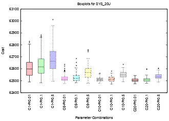
to 3 show in the x-axis the parameter combinations and the y-axis indicates the objective function values for each problem. We can see that better results are reached with the lowest probability value and the highest population size. So, C=5and Pr=0.01 were used to compare the results got by IA EDP S with those produced by other approaches.

Considering the lowest number of objective function evaluations used by the other approaches (see [2]) we take as maximum number of function evaluations, 1000, 40000, 3000, 20000 and 20000 for SYS 3U, SYS 18U, SYS 6U, SYS 15U and SYS 20U, respectively. Also, we setǫ=0.1 for those problems which consider loss transmission (e.d. SYS 6U, SYS 15U and SYS 20U).

8194 8195 8196 8197 8198 8199 8200 8201

C1-Pr0.01 C1-Pr0.1 C1-Pr0.5 C5-Pr0.01 C5-Pr0.1 C5-Pr0.5 C10-Pr0.01 C10-Pr0.1 C10-Pr0.5 C20-Pr0.01 C20-Pr0.1 C20-Pr0.5

Cost

Parameter Combinations Boxplots for SYS_3U

25420 25430 25440 25450 25460 25470 25480 25490 25500 25510

C1-Pr0.01 C1-Pr0.1 C1-Pr0.5 C5-Pr0.01 C5-Pr0.1 C5-Pr0.5 C10-Pr0.01 C10-Pr0.1 C10-Pr0.5 C20-Pr0.01 C20-Pr0.1 C20-Pr0.5

Cost

Parameter Combinations Boxplots for SYS_18U

Fig. 1.Box plots for the test problems with the best parameters combination

15440 15450 15460 15470 15480 15490 15500 15510 15520 15530 15540

C1-Pr0.01 C1-Pr0.1 C1-Pr0.5 C5-Pr0.01 C5-Pr0.1 C5-Pr0.5 _C10-Pr0.01 C10-Pr0.1 C10-Pr0.5 _C20-Pr0.01 C20-Pr0.1 C20-Pr0.5

Cost

Parameter Combinations Boxplots for SYS_6U

32650 32700 32750 32800 32850 32900 32950 33000 33050 33100

C1-Pr0.01 C1-Pr0.1 C1-Pr0.5 C5-Pr0.01 C5-Pr0.1 C5-Pr0.5 _C10-Pr0.01 C10-Pr0.1 C10-Pr0.5 _C20-Pr0.01 C20-Pr0.1 C20-Pr0.5

Cost

Parameter Combinations Boxplots for SYS_15U

Fig. 2.Box plots for the test problems with the best parameters combination

5

Comparison of Results and Discussion

62400 62500 62600 62700 62800 62900 63000 63100

C1-Pr0.01 C1-Pr0.1 C1-Pr0.5 C5-Pr0.01 C5-Pr0.1 C5-Pr0.5

C10-Pr0.01 C10-Pr0.1 C10-Pr0.5 C20-Pr0.01 C20-Pr0.1 C20-Pr0.5

Cost

Parameter Combinations Boxplots for SYS_20U

Fig. 3.Box plots for the test problem with the best parameters combination

due to space restrictions. For all the test problems, our proposed IA EDP S found feasible solutions in all the runs performed.

Problems which do not consider transmission loss, rate ramp limits or pro-hibited zones, i.e., SYS 3U and SYS 18U, do not seem to be a challenge for IA EDP S. The standard deviations obtained by IA EDP S are lower than 1. Additionally, the problem dimensionality does not seem to affect the perfor-mance of our proposed approach either.

For problems which consider transmission loss, rate ramp limits and prohib-ited zones, SYS 6U a and SYS 15U, the standard deviations increase with the problem dimensionality.

For the only problem which considers transmission loss but not rate ramp lim-its or prohibited zones, SYS 20U, the standard deviation is lower than SYS 15U’s standard deviation.

Table 2.Results obtained by IA EDP S

Problem Best Worst Mean Median SD. Ev.

SYS 3U 8194.3561 8194.3784 8194.3597 8194.3584 0.004 987.16 SYS 18U 25429.8005 25433.0655 25430.9312 25430.8415 0.614 35103.15 SYS 6U 15442.8962 15455.2466 15444.3082 15443.6071 1.877 1490.62 SYS 15U 32700.2971 32865.2657 32763.5364 32758.1897 35.765 18321.5 SYS 20U 62476.1186 62636.5875 62522.3703 62513.2753 30.371 8151.36

(some-thing that was not possible in our case, since we do not have the source code of several of them). Clearly, in our case, the emphasis is to identify which approach requires the lowest number of objective function evaluations to find solutions of a certain acceptable quality.

However, the running times are also compared in an indirect manner, to give at least a rough idea of the complexities of the different algorithms considered in our comparative study. For all test problems IA EDP S found the best cost in the lowest time. Except for SYS 3U, where fast-PSO just required 0.01 second and IA EDP S spent 0.18 seconds to find the best solution.

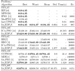
Table 3 summarizes the performance IA EDP S with respect to that of the other methods. As shown in Table 3, considering the best cost found, IA EDP S outperforms all other approaches. Considering running times, IA EDP S requires less than one second to find solutions with an acceptable quality for SYS 3U and SYS 6U. It requires less than 1.4 second for SYS 15U and SYS 18U. And it requires less than 2.1 second for SYS 20U.

We could not found an approach that report feasible solutions for SYS 20U, so IA EDP S obtained the best results.

Table 3.Comparison of results. The best values are shown inboldface.

Problem/

Algorithm Best Worst Mean Std. Time(s) Ev.

SYS 3U

IEP[10] 8194.35 - - - -

-MPSO[9] 8194.35 - - - -

-IPSO [11] 8194.35 - - - 0.42 3000

ModPSO [12] 8194.40 - - - -

-fast-CPSO[4] 8194.35 - - - 0.01 3000

IA EDP S 8194.35 8194.37 8194.35 0.004 0.18 987 SYS 18U

ICA-PSO [13] 25430.16 25462.34 25440.89 - 18.585 40000 IA EDP S 25429.80 25433.06 25430.93 0.614 1.168 35103 SYS 6U

IHS[7] 15444.30 - 15449.86 4.531 - 100000

BBO [3] 15443.0915443.09 15443.09 - - 50000 ICA-PSO[13] 15443.24 15444.33 15443.97 - - 20000 IA EDP S 15442.89 15455.24 15444.30 1.877 0.828 1490 SYS 15U

CCPSO[8] 32704.4532704.45 32704.45 0.0 16.2 30000

MDE[1] 32704.9 32711.5 32708.1 - - 160000

SA-PSO [5] 32708.00 32789.00 32732.00 18.025 12.79 20000 IA EDP S 32700.29 32865.26 32763.53 35.76 1.328 18321 SYS 20U

6

Conclusions and Future Work

This paper presented an adaptation of an algorithm inspired on the T-Cell model of the immune system, called IA EDP S, which was used to solve economic dispatch problems. IA EDP S is able to handle the five types of constraints that are involved in an economic dispatch problem: power balance constraint with and without transmission loss, operating limit constraints, ramp rate limit constraint and prohibited operating zones.

At the beginning, the search performed by IA EDP S is based on a simple differentiation operator which takes an infeasible solution and modifies some of its decision variables by taking into account their constraint violation. Once the algorithm finds a feasible solution, a redistribution power operator is applied. This operator modifies two decision variables at a time, it decreases the power in one unit, and it selects other unit to generate the power that has been taken. The approach was validated with five test problems having different charac-teristics and comparisons were provided with respect to some approaches that have been reported in the specialized literature. Our results indicated that di-mensionality increases standard deviations when the same types of constraints are considered but prohibited zones have more impact on the performance than dimensionality. Our proposed approach produced competitive results in all cases, being able to outperform the other approaches while performing a lower number of objective function evaluations than the other approaches.

As part of our future work, we are interested in redesigning the redistribution operator in order to maintain the solutions’ feasibility when a problem involves prohibited operating zones.

References

1. N. Amjady and H. Sharifzadeh. Solution of non-convex economic dispatch prob-lem considering valve loading effect by a new modified differential evolution algo-rithm. International Journal of Electrical Power and Energy Systems, 32(8):893– 903, 2010.

2. V.S. Aragon, S.C. Esquivel, and C.A. Coello Coello. An immune algorithm with power redistribution for solving economic dispatch problems.Information Sciences, 295(0):609 – 632, 2015.

3. A. Bhattacharya and P.K. Chattopadhyay. Biogeography-based optimization for different economic load dispatch problems.IEEE Transactions on Power Systems, 25(2):1064–1077, 2010.

4. Leticia Cecilia Cagnina, Susana Cecilia Esquivel, and Carlos A. Coello Coello. A fast particle swarm algorithm for solving smooth and non-smooth economic dispatch problems. Engineering Optimization, 43(5):485–505, 2011.

5. Cheng-Chien Kuo. A novel coding scheme for practical economic dispatch by mod-ified particle swarm approach. IEEE Transactions on Power Systems, 23(4):1825– 1835, 2008.

7. V.R. Pandi, K.B. Panigrahi, M.K. Mallick, A. Abraham, and S. Das. Improved harmony search for economic power dispatch. InHybrid Intelligent Systems, 2009. HIS ’09. Ninth International Conference on, volume 3, pages 403–408, 2009. 8. J.-B. Park, Y.-W. Jeong, J.-R. Shin, and K.Y. Lee. An improved particle swarm

optimization for nonconvex economic dispatch problems. IEEE Transactions on Power Systems, 25(1):156–166, 2010.

9. Jong-Bae Park, Ki-Song Lee, Joong-Rin Shin, and K.Y. Lee. A particle swarm optimization for economic dispatch with nonsmooth cost functions.Power Systems, IEEE Transactions on, 20(1):34–42, 2005.

10. Y. M. Park, J. R. Won, and J. B. Park. A new approach to economic load dis-patch based on improved evolutionary programming.Eng. Intell. Syst. Elect. Eng. Commun., 6(2):103–110, June 1998.

11. P. Sriyanyong, Y.H. Song, and P.J. Turner. Particle swarm optimisation for op-erational planning: Unit commitment and economic dispatch. In KeshavP. Dahal, KayChen Tan, and PeterI. Cowling, editors,Evolutionary Scheduling, volume 49 of Studies in Computational Intelligence, pages 313–347. Springer Berlin Heidelberg, 2007.

12. S. Siva Subramani and P. Raja Rajeswari. A modified particle swarm optimization for economic dispatch problems with non-smooth cost functions. International Journal of Soft Computing, 3(4):326–332, 2008.

13. J.G. Vlachogiannis and K.Y. Lee. Economic load dispatch a comparative study on heuristic optimization techniques with an improved coordinated aggregation-based pso. IEEE Transactions on Power Systems, 24(2):991–1001, 2009.