MPRA
Munich Personal RePEc Archive
A composed error model decomposition
and spatial analysis of local
unemployment
Jaime Cu´ellar Mart´ın and ´
Angel L. Mart´ın-Rom´
an and
Alfonso Moral
University of Valladolid, University of Valladolid, University of
Valladolid
19 June 2017
Online at
https://mpra.ub.uni-muenchen.de/79783/
A composed error model decomposition and
spatial analysis of local unemployment
Jaime Cuéllar-Martín
Ángel L. Martín-Román
1Alfonso Moral de Blas
Department of Economic Analysis
University of Valladolid
ABSTRACT
The differences in the regional unemployment rates, as well as their formation mechanism and persistence, have given rise to a great number of papers in the last decades. This work contributes to that strand of literature from two different perspectives. In the first part of our work, we follow the methodological proposal established by Hofler and Murphy (1989) and Aysun et al. (2014). We make use of an estimation of a stochastic cost frontier to breakdown the Spanish provincial effective unemployment (NUTS-3) in two different components: first one associated with aggregate supply side factors, and the other one more related to the aggregate demand side factors. The second part of our research analyzes the existence of spatial dependence patterns among the Spanish provinces in the effective unemployment and in both above mentioned components. The decomposition performed in the first part of our research will let us know the margin that the policymakers have when they deal with unemployment reductions by means of aggregate supply and aggregate demand policies. Finally, the spatial analysis of the unemployment rates amongst the Spanish provinces can potentially have also significant implications from an economic policy viewpoint since we find that there are common formation patterns or clusters of unemployment.
Key Words: Unemployment, Local labor markets, spatial dependence.
JEL Codes: E24, J64, R11.
1 Corresponding author (e-mail address: [email protected])
1.
Introduction
In recent years the number of scientific works analysing local and regional disparities in unemployment rates has grown substantially, underpinning the importance of the topic. In this kind of analysis, the case of Spain proves particularly appealing given the regional disparities in the unemployment rate and the extent to which these have persisted over the years (Jimeno and Bentolila, 1998; Bande et al. 2008; Romero-Ávila and Usabiaga, 2008; Sala y Trivín, 2014).
The present work seeks to go a step further in this field of literature from a double perspective: firstly, unemployment rates are broken down into two components, one associated with factors related to aggregate supply and the other explained using economic factors related to aggregate demand. The econometric technique used is the so-called the stochastic frontier methodology, which means an innovation in this kind of analysis for the
Spanish case. This methodology is applied to a database which provides information on the
50 Spanish provinces for the period between 1984 and 20122. Pinpointing the components
that make up the effective unemployment rate proves important for a number of reasons, in that it sheds light on which factors impact on the effective unemployment rate most and which exert the greatest influence on its evolution over time. Furthermore, said decomposition may prove extremely useful vis-à-vis gaining an insight into how much manoeuvring space the policymakers have when devising and implementing economic policy measures at a territorial level.
The second part of the work tests whether there is any spatial dependence between provincial unemployment figures. In order to undertake this analysis, we first examine the existence of spatial dependence at an overall level based on the values of Moran’s I statistic (Moran, 1950). These statistics allow us to compare the existence or lack of correlation at a global scale but do not allow us to evaluate the local structure of spatial correlation. For this reason, we go one step further and build local statistics LISA (“Local Indicators of Spatial Association”)3. It is thus possible to decompose the global statistic and to locate any
possible clusters associated to the effective provincial unemployment rate. This part of the research is complemented by spatial analysis of the components of unemployment obtained: those linked to aggregate supply and to aggregate demand. As a measure of robustness, various alternative definitions of neighborhood are also applied. Finally, this research includes a list of various theoretical effects to explain the possible existence of spatial dependence between the effective provincial unemployment rates, and between its two components.
The remainder of the work is organised as follows. Section 2 offers a review of the literature related to the topic in hand. Section 3 examines the conceptual framework on which the decomposition of effective provincial unemployment rates is based. Section 4 sets out the method used in the econometric analysis. Section 5 provides a brief description of the databases employed and defines the variables used. Section 6 presents and explains the results, both with regard to the decomposition of effective provincial unemployment rates as well as in the evolution and spatial analysis of their components. Finally, section 7 sums up the most relevant conclusions to emerge from the research and posits some economic policy measures.
2.
State of the question
Since the present work presents two clearly differentiated blocks, the bibliographical review also is conducted in two distinct sub-sections. A first sub-section thus addresses studies which, from the perspective of unemployment decomposition, adopt the stochastic frontier approach, whilst the second sub-section includes some of the research which has explored the issue of regional unemployment from a range of perspectives.
2 The 50 Spanish provinces correspond to the third level (NUTS-3) of the Nomenclature of Territorial Units for statistics. For
further information concerning the concept of NUTS, see: http://ec.europa.eu/eurostat/web/nuts/overview.
2.1
Decomposition of unemployment
Decomposing unemployment into its different components is a common theme in economic
literature, and a variety of techniques has been employed for this purpose4. One of the most
widely used options involves applying univariate statistical filters5. Few works, however,
adopt the econometric approach of stochastic frontiers.
One of the pioneering works in this technique was Warren (1991). Said work uses the stochastic frontiers technique to decompose the unemployment rate, also drawing on
information concerning vacancies6. Using the number of vacancies and the number of
persons unemployed, an efficient matching function is estimated through an upper stochastic frontier. Based on this, the author determines the frictional component of unemployment for the USA for the period stretching from April 1969 to December 1979. Another work which follows the same line is that of Bodman (1999) who takes the model set out by Warren (1991) as a starting point, and models the inefficiency term of the error following the proposal of Battese and Coelli (1995).
One work which follows a closer line to the approach adopted in the present research is that of Hofler and Murphy (1989). The authors posit a model for ascertaining the frictional component of unemployment in which the unemployment rate is split into one frictional component and another which captures an excess of aggregate supply in the labour market. Hofler and Murphy (1989) estimate a stochastic cost frontier using the unemployment rate of the fifty US states for the period 1960-1979. They find great variability in the frictional component of unemployment and an increase for most states during the period analysed.
Finally, Aysun et al. (2014) propose a method for estimating the structural component of the unemployment rate for the USA from 1960 to 2010. This article merges elements from the three previous studies. A very similar approach to the one employed in Warren (1991) is initially used to extract frictional unemployment. Secondly, and by applying a stochastic cost frontier, they estimate the structural component of the unemployment rate by using a specification of the expectation augmented Phillips curve. By adopting this procedure, Aysun et al. (2014) calculate a measure of structural unemployment which is always below the effective component.
2.2
Analysis of unemployment from a regional perspective
In recent years, economists have displayed increasing interest in how labour markets function at a regional level, which has given rise to a large number of studies. Overman and Puga (2002) report results for some European regions for the period 1986-1996. Their study points to an ever-growing polarisation between “high” unemployment and “low” unemployment regions, depending on the spatial influence exerted by their neighbours. Patacchini and Zenou (2007) explore the existence of imbalances in unemployment for the UK and find a strong positive spatial dependence between relative local unemployment rates. Their study points to an increase in spatial dependence over time, which is explained to a large degree by flows of individuals between local areas.
Cracolici et al. (2007) adopt a very similar approach to Overman and Puga (2002). The main innovation provided in their work is its contribution to the empirical evidence concerning spatial and temporal persistence for the 103 Italian provinces between 1998 and 2003. The explanation given by the authors for this process of “clustering” is due to factors which fit in with the hypothesis of imbalance (Marston, 1985) for 1998. However, for 2003 the factors leading to this “clustering” are far more closely linked to elements related to the equilibrium hypothesis (Marston, 1985). Finally, they stress the influence of labour demand
4 The work of Fabiani and Mestre (2000) sets out some of these techniques applied to the case of the European Union.
5 The Hodrick-Prescott filter (Hodrick and Prescott, 1997) and the Baxter-King filter (Baxter and King, 1999) are some of the most
widely used in the literature.
6 It is precisely this use of information concerning vacancies which makes it impossible for the present paper to adopt the technique
factors as the key dynamic underlying the polarisation of unemployment between provinces in the north (“low” unemployment) and the south (“high” unemployment).
Filiztekin (2009) reports a strong spatial dependence of regional unemployment rates. The author finds that the factors which most contribute to shaping the distribution of unemployment are the growth in employment in 1980 and human capital in the year 2000. Basile et al. (2009) also underpin the role played by the imbalance between labour supply and demand as well as the “brain drain” which occurs through migration. These two elements prove to be the most determinant when accounting for the provincial differences in unemployment in Italy in the period 1995-2007.
Kondo (2015) conducts a slightly different analysis to those employed in the above-mentioned works. His research provides empirical evidence related to the persistent unemployment rates in certain Japanese municipalities over the period 1980-2005. Using spatial econometrics, the author finds clusters in municipal unemployment rates with positive spatial dependence. On the other hand, the study shows the existence of very important differences in terms of sex and age with regard to the spatial dependence of unemployment rates. It also reflects how municipalities with “high” unemployment tend to remain in this situation throughout the time period studied. Halleck Vega and Elhorst (2016), employs a “Simultaneous model” and try to account for serial dynamics, spatial dependence and common factors using data on overall unemployment for 12 regions of Netherlands over the period 1973-2013. They find empirical evidence about the existence of strong and weak spatial dependence in their data.
As regards the analysis of differences in the issue of unemployment between the various Spanish regions, the works of López-Bazo et al. (2002, 2005) use exploratory techniques at the spatial level merged with classical spatial regression analysis. Both studies highlight the strong polarisation of Spanish provinces into two groups (“high” and “low” relative unemployment). Adopting a different perspective, Huertas et al. (2006) apply the model introduced in the work of Blanchard and Katz (1992) to determine the degree of persistence of unemployment in Andalusia and Extremadura over the period spanning from the third quarter of 1976 to the fourth of 2004. The authors conclude that a positive shock in labour demand at the provincial level triggers a permanent impact on labour force participation in Andalusia and the unemployment rate in Extremadura, and highlighting the scant worker mobility in the two regions.
The study by Bande et al. (2008) focuses on the 17 autonomous communities (NUTS-2) in Spain over the period 1980-2000. The findings point to a greater disparity of relative unemployment rates in Spanish autonomous communities during upturns, and to a reduction thereof during periods of economic recession. The explanation given is based on a strong “mimicking effect” in the wage bargaining mechanism in Spanish regions. Said effect is heightened due to the change in this mechanism’s level of centralisation and coordination, giving rise to a worsening, in terms of unemployment of regions with lower productivity.
More recent works such as those of Azorín (2013) provide conclusions evidencing a strong polarisation which is reflected in the group of Spanish provinces displaying “high” unemployment rates in the southern half of the country and a group of provinces with noticeably “low” unemployment rates in the northern half of the country. López-Bazo and Motellón (2013) adopt an approach based on the use of microdata for Spanish autonomous communities in 1999, 2004 and 2009. Their study finds that regional disparities between unemployment rates persist over time. The authors also highlight the determinant role played by variables related to the educational features of the population in regions with “high” and “low” unemployment.
3.
Conceptual framework
presents some of the social and economic phenomena found in the literature, and which contribute to the formation of clusters in unemployment.
3.1.
Components of the effective unemployment rate
In the economic literature has been common to break down aggregate unemployment into
different components, as shown in equation (1)7:
= + +
(1)
where is the effective unemployment rate in province i at time t; is the frictional
unemployment rate; is the structural unemployment rate and, finally, represents
the cyclical unemployment rate.
In line with the “job search theory”, the existence of asymmetric or imperfect information amongst job-seekers and employers means that labour market matching takes some time and that there will always be some people unemployed. This is what leads to
frictional unemployment8. Structural unemployment is commonly assumed to be linked to
aggregate supply factors (as opposed to , which is considered to be linked to aggregate
demand factors)9. Imbalances between labour supply and demand cause situations in which
there are both people unemployed and unoccupied vacancies in firms, thus leading to
unemployment10.
Based on the above, macroeconomic literature has established that the sum of frictional unemployment and structural unemployment gives rise to the so-called “natural
rate of unemployment” or “NRU”11. This “natural rate of unemployment” acts as
equilibrium unemployment in the long or medium term for the unemployment observed and is expressed formally through equation (2):
= + (2)
where is the natural rate of unemployment in province i at time t.
The natural rate of unemployment is related to aggregate supply determinants at a macroeconomic level, and explains that there will always be “some” level of
unemployment12. Nevertheless, during times of “low” economic growth, or during recessions
sparked by adverse demand shocks, aggregate demand would also be “insufficient”13. As a
result, a further element, which we already identified as cyclical unemployment, must be added to the previous factors. This idea may be expressed by means of equation (3):
= + (3)
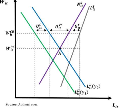
Figure 1 depicts a very simple labour market graphically illustrating what was pointed out previously. The curve is the labour force and displays a positive slope. This is because, as the market wage increases ( ), more individuals join the labour market given that their “static” reservation wage (or that of the choice model between consumption and leisure) is lower than the market wage.
7 Even in textbooks like Krugman et al. (2011), this classification can be found.
8 This theory was developed by Mortensen (1970) and McCall (1970). See Lippman and McCall (1976a; 1976b), Mortensen (1986)
and Mortensen and Pissarides (1999), for a review of the issue in question. One recent example of this type of literature is the works of Tatsiramos and van Ours (2012, 2014).
9 The same happens with the frictional component ( ).
10 These imbalances arise as a result of a certain amount of institutional rigidity, linked to the downward rigidity of wages
(minimum wage, collective bargaining, etc.) or employment protection, amongst others. Other factors which also impact strongly on the imbalances between supply and demand are: inflow and outflow in the labour market, labour force skills, low labour productivity, the industry composition of employment or the demographic structure of the population, to name but a few (Jackman y Roper, 1987; Blanchard y Jimeno, 1995; Blanchard, 2017).
11 Rogerson (1997) provides a number of explanations, definitions and nomenclature of the concept.
12 Even when macroeconomic conditions reach optimal levels and there are no problems of insufficient aggregate demand. 13 Due, for example, to a fall in consumer or business confidence. A contractive monetary policy or a cut in public spending might
The curve shows the effective labour supply. The difference between and establishes that not all active workers are immediately available for work. As the market wage increases and rises above the “dynamic” reservation wage (or that of the job search theory), more workers will accept the jobs they find. For this reason, the distance between and is lower for higher wages. This difference between the two previously mentioned curves is frictional unemployment ( ).
Figure 1 also shows two situations of the demand for employment, depending on
how aggregate production stands. Situation ( ) represents economic expansion, whereas
situation ( ) reflects an economic recession. Point “A” shows how, in a situation in which
production is booming and the market wage is at its equilibrium level, with a ,( )
demand of work, there are unemployed workers due to the presence of frictional unemployment.
Figure 1. Frictional, structural and cyclical unemployment
In addition, the existence of a collective bargaining system impacts on the
mechanism for establishing wages by fixing a “collective bargaining” ( ) wage which is
above the competitive equilibrium wage ( ). This is one example of institutional
inflexibility which leads to an excess of labor supply, and triggers structural unemployment ( )14. As in the previous case, some structural unemployment would also exist even if
demand for work were , ( ), which is associated to an economic boom. Several studies
(Bentolila and Jimeno, 2003; Simón et al., 2006; Bande et al., 2008) point out that the “inflexibility” of wages prevents these from acting as an equilibrium mechanism in the
Spanish labour market15. In line with this, “via price” adjustment does not function
“correctly”, thus leading to adjustments in the labour market occurring “via quantity16.
14 Elhorst (2003) cites some works which have explored the effect of collective bargaining on unemployment. Most report a positive
effect, which would seem to confirm the previously posited hypothesis.
15 For a more comprehensive explanation of the issue, see Jimeno and Bentolila, (1998), Garcia-Mainar and Montuenga-Gomez
(2003), Maza and Moral-Arce (2006), Maza and Villaverde (2009) or Bande et al. (2012).
16 Cazes et al. (2013) show how in Spain, during the Great Recession, labour market adjustment mainly occurred through the
external margin of adjustment (layoffs and downsizing) in the labour market.
A
( )
( )
Cyclical unemployment ( ) is the final component in equation (1). Insufficient aggregate demand leads to a drop in sales in business. This in turn, sparks a reduction in labour demand due to the fact that it is derived demand. In figure 1, cyclical unemployment
is reflected in the horizontal distance between curves ( ) and ( ). This kind of
unemployment may be corrected in the short term by applying expansive aggregate demand policies. At this point, an important clarification should be made concerning the aims of the present work between the notion of the natural rate of unemployment (NRU) and the non-accelerating inflation rate of unemployment (NAIRU). The two concepts are often used indistinctly, and yet various studies question whether the NRU and NAIRU are interchangeable concepts.
Tobin (1997) establishes that the NAIRU and NRU are not one and the same. On the one hand, the NAIRU reflects a relation at a macroeconomic level, whereas the NRU is a rate of unemployment equilibrium influenced by institutional demographic features of the economy, and refers to aspects that are much more microeconomic in nature (Grant, 2002). The NAIRU is associated with negative cyclical unemployment at certain periods (when the inflation rate rises). This leads to the sum of frictional unemployment and structural unemployment being greater than effective unemployment. In our view, this situation is somewhat “striking” for labour economics models which tend to have more of a microeconomic basis. These models consider that effective unemployment comprises three components of equation (1), although none of them should be negative (in other words,
≥ 0; ≥ 0; ≥ 0). In the current work, we are more interested in the concept of NRU than NAIRU, since inflation plays no relevant role here. Based on the above, we seek to measure how much unemployment remains when there is no problem of insufficient aggregate demand. It is thus possible to quantify how much unemployment is attributable to aggregate supply factors and how much to aggregate demand factors for each province and year. Said minimum level of unemployment can be obtained as a stochastic cost frontier based on estimating a composite error econometric model. As a result, we partially follow the proposal put forward by Hofler and Murphy (1989) and more recently by Aysun et al. (2014), set out earlier.
From an applied standpoint, NRU is seen as medium term equilibrium unemployment that depends on factors which the literature has considered as determinants
of frictional and structural unemployment, (vector of variables ). Therefore, the
minimum natural or “efficient” unemployment would be a function of that vector of
variables ( = ( )). Any deviations with regard to said minimum would be seen as
inefficiencies and would be the result of insufficiencies in aggregate demand. In other
words, cyclical unemployment is modelled as a non-negative disturbance = ≥ 0.
Finally, and assuming linearity ( ( ) = ), the estimable version of (1) would be:
= + +
(4)
where is a conventional random disturbance. In equation (4), it is implicitly assumed that cyclical unemployment has a minimum value equal to 0. Should the opposite prove to be the case, situations might arise in which the natural rate of unemployment was higher
than actual effective unemployment, as already pointed out17. Put differently, the
component acts as a lower limit or frontier for effective unemployment ( ≥ ).
3.2.
Factors generating spatial dependence in unemployment
In our work, we also try to test for the presence of spatial dependence in the effective unemployment rates and in its two components. For this reason, this section explores some of the phenomena whose characteristics display certain social and economic features that help us to explain why similar rates of unemployment can be found in certain neighbouring areas.
17 In the papers by Revoredo-Giha et al. (2009), Sav ( 2012) or Duncan et al. (2012), it is assumed that the “frontier cost” is the
1. “Peer Effect”: The first of these phenomena is the so-called “peer effect”, which, according to Dietz (2002), emerges when “the behaviour of an individual has a direct
influence on the behaviour of every other individual in the neighborhood”18
.
Theinfluence of the previous effect may be seen through two different channels:
1.1 “Social Network Peer Effect”: The first relates to the effect caused by individuals’
“social networks” or “employment networks”. From this standpoint, in areas of “low” unemployment, most people join networks whose members are working. Nevertheless, in areas of “high” unemployment, networks tend to comprise people who are out of work. The employment situation of the members of the “social network” which a person forms part of affects the latter’s likelihood of finding a job, positively in the case of areas of “low” unemployment and negatively in areas of “high” unemployment (Topa, 2001; Conley and Topa, 2002; Calvo-Armengol and Jackson, 2004; Cingano and Rosolia, 2012).
1.2 “Social Cost Peer Effect”: The second channel addresses the social and psychological
cost of being unemployed. In areas of “low” unemployment, the psychological and social cost for those who are unemployed is high since most of their neighbours are working. This situation drives unemployed persons to engage in a more intense job search (Hedström et al. 2003), thereby enhancing their chances of finding work. In contrast, in areas of “high” unemployment, the psychological and social cost for those who are unemployed is lower. This is because the reference group (neighbours) are in a similar situation (Hedström et al. 2003; Clark, 2003), which discourages a more intense job search.
These two channels generate a positive spatial dependence in unemployment rates and the persistence of “high” (“low”) unemployment (Calvo-Armengol and Jackson, 2004; Bramoullé and Saint-Paul, 2010)19.
2. “Commuting Effect”: Another phenomenon which yields the creation of spatial
clusters and spatial dependence in general terms, concerns the geographical mobility of workers around the areas adjacent to where they live. The “commuting effect" leads to the unemployment rates in nearby or adjacent areas displaying a certain spatial
dependence20. This assumption is justified since individuals seek employment and work
in the closest areas where they live. This helps create an interrelation amongst areas and as a consequence we find that unemployment rates could be spatially correlated (Patacchini and Zenou, 2007).
3. “Migration Effect”: The next aspect concerns people’s decision to move to nearby
provinces or regions rather than to those which are further away. This decision to move away is closely linked to uncertain job prospects (based on imperfect information) and to the growing cost as distance increases (Tassinopoulos and Werner, 1999)21. Such
factors cause a greater spatial dependence between nearby areas than between areas which are further apart, given that the benefit derived from migrating diminishes as distance increases.
4. “Spillover Effect”: The fourth effect is the so-called “Spillover Effect”. This
phenomenon arise when the effects (in an economic sense) generated in one singular area, have been caused by the actions occurred in other nearest areas (neighbouring areas). As we said before, there is an economic influence amongst the neighbouring
18 This type of effect has also been used in microeconomics under the name “Bandwagon effect”. See Topa and Zenou (2015) and
Ioannides and Datcher Loury (2004) for a more detailed explanation.
19 Topa (2001) and Conley and Topa (2002) show how the spatial patterns evident in unemployment are due to the exchange of
information amongst individuals through different channels (geographical, ethnical etc.).
20 Elhorst (2003) refers to commuting as one of the factors to be taken into account when explaining regional unemployment rates. 21 The growing cost as distance increases not only concerns purely monetary costs (transport costs, accommodation costs) but also
areas, which can contribute to developing common patterns. A large variety of spillover effects has been developed by the literature, but in our case, we will focus on two specific channels22:
4.1 “Standard Spillover Effect”: This effect is caused by each area’s productive
structure. There are areas which “spill over” activity towards neighbouring locations, thereby generating similarities between their industrial composition despite them being spatially different areas. This gives rise to major trade links that bring about an analogous productive specialisation between neighbouring areas. The previous situation generates resemblances between their labour market
structures that might also lead to them displaying similar unemployment rates23.
4.2 “Fiscal Policy Spillover Effect”: The latter phenomenon concerns the existence of a
certain spillover effect caused by the action of a fiscal policy that might give rise to aggregate demand shocks, in the short run, in areas adjacent to those in which the policy has been applied, also impacting on its unemployment rate24. Applying an
expansive fiscal policy (contractionary) in a given area “i” causes a positive aggregate demand shock (negative) in neighbouring province “j”, thus contributing
to reducing (increasing) unemployment in both areas due to their spatial relation25.
The previous effect depends heavily on the area in which it is applied, the type of the fiscal policy and, amongst others, the sign of the policy (expansive or contractionary). Based on this, the effects generated by this type of spillover effect could be less redundant in time and space. In other words, it could be expected that the effects exerted of the “Fiscal Policy Spillover Effect” will occur in the short run and with a great variability in the neighbouring areas. Finally, we can say that a certain positive spatial dependence might be expected and therefore a similarity between unemployment levels in adjacent areas.
4.
Methodology
As commented on in section 3.1, the decomposition of the unemployment rate posited in the present work is based on the concept of the “NRU” and on the non-negativity of its components. Given this assumption, the method best suited to our goals is that known as stochastic frontiers. This technique first appeared in the works of Aigner et al. (1977) and Meeusen and van Den Broeck (1977) and has become widespread in efficiency analysis when seeking to obtain maximum production or minimum costs. Its practical application in the cost version allows a value to be obtained which acts as a lower limit for the target variable26. This minimum value is identified in the present work as medium (long) term
equilibrium unemployment, and the deviation from this minimum is considered to be an inefficiency associated to insufficient aggregate demand. In more analytical terms, the lower frontier coincides with the sum of frictional unemployment ( ) and structural
unemployment ( ), in other words, the natural rate of unemployment ( ). The
difference between this and the effective unemployment rate ( ) is referred to as cyclical unemployment ( ).
As pointed out before, the natural rate of unemployment depends on variables which affect structural and frictional unemployment, such that it may be expressed as
22 See among others del Barrio-Castro et al., 2002; Moreno et al., 2005; López-Bazo et al., 2005.
23 There might be adjacent areas which display determinant economic features that function poorly. Here, the “spill over” which
occurs in adjacent areas proves relatively inefficient from the economic standpoint, generating a negative Spillover Effect. For example, large-scale redundancies in a given area might trigger depressive economic effects in adjacent areas. See Martin (1997).
24See Solé-Ollé (2003); Brueckner (2003); Costa et al., (2015); Ríos et al., (2017) and López et al., (2017) among others to provide a
detailed explanation about similar effects in the public sector.
25 For example, increasing public spending on infrastructures in area “i” gives rise to a reduction in unemployment both in area “i”
and the adjacent area “j”, leading to the unemployment rates being similar in the two areas. In the case of a negative aggregate demand shock (for example, a cut in public spending), the opposite would occur. In other words, there would be an increase in unemployment in the two neighbouring areas.
= ( ). Equation 5 shows the econometric specification of this natural rate of
unemployment, assuming linearity in the model27:
= + (5)
where is a vector of the coefficients, is a vector of explanatory variables and is a
random error of mean 0 and variance . acts as a theoretical no observed lower bound.
Our information comes from the effective unemployment rate, which is greater than or
equal to this component ( ≥ ). In this way, the effective unemployment rate may be
represented as the sum of the natural rate of unemployment and a non-negative random disturbance ( ) which is identified with cyclical unemployment ( ) through the following expression:
= + (6)
where is an error term expected to be positive and independently distributed taking the
form ( , ). The strategy adopted in the present research is based partially on the
approach presented by Aysun et al. (2014), where cyclical unemployment is also felt to have a minimum value equal to 0. By merging equations (5) and (6), expression (7) is obtained which coincides with equation (4) in section 3.1:
= + (7)
where: = +
As a result, in accordance with expressions (4) and (7), we are dealing with an econometric specification that has a composed error. In such instances, and provided that the disturbances and regressors are independent, the Ordinary Least Squares estimation (OLS), provides non-biased, consistent and efficient estimators. Nevertheless, there is inconsistency in the constant term and it is not possible to separate the variances of the two
disturbances
.
This causes problems because, in order to conduct tests which validate theexistence of inefficiency, it is necessary to have information concerning the variance associated to each disturbance. In order to overcome all of these deficiencies, it is necessary to resort to other more appropriate estimation methods such as maximum likelihood estimation. It should, however, be borne in mind that in order to carry out this kind of estimation, a distribution for each of the two error components (Jondrow et al., 1982) must be assumed. In the case of the component , there would be no problem, since there seems to be a strong consensus in the empirical literature in the sense that said component
is distributed in the form (0, ). The main problem arises when we need to consider the
distribution of the term 28. In this case, and as in Hofler and Murphy (1989) and Aysun et
al. (2014), we opt to use semi-normal distribution.
Having decomposed the effective provincial unemployment rate, the next step in the econometric analysis is to study whether or not there is spatial dependence in the effective provincial unemployment rate and in each of its components. In order to be able to identify these spatial patterns, a matrix of weights indicating what neighborhood criterion we are using must first be defined. The literature has used various alternatives such as the existence of a common frontier, the matrix of K nearest neighbours (knn) or matrices of distances. After choosing a criterion, the existence of spatial dependence may be determined by using a given overall spatial dependence statistic. In the current work, we use the statistic known as Moran’s I (Moran, 1948) which is defined in line with expression (8)29:
27 The lack of information which is sufficiently ample and comparable over time concerning existing vacancies in the labour market
makes it extremely difficult to extract the frictional component ( ) in line with the approach adopted in Warren (1991), Bodman (1999) and Aysun et al. (2014), such that said component is estimated together with structural unemployment.
28 In this case, several distributions have been proposed in the econometric literature: Normal truncated (Stevenson, 1980),
Semi-Normal (Aigner et al., 1977), Exponential (Meeusen and van Den Broeck, 1977) and Gamma (Greene, 1990).
= ∗ ∑ ∑ (( ̅)̅) ̅ (8)
where is the sample size, refers to the components of the spatial weights matrix,
represents the value of variable in province , is equal to ∑ ∑ and finally, ̅
corresponds to the sample mean of variable . This statistic takes values ranging between 1 and -1, such that there is positive spatial dependence when its values are close to 1, and negative when they approach -1 (values close to zero indicate the absence of spatial dependence). The existence of positive spatial dependence means that areas with “high” (“low”) values of the target variable are surrounded by others which also display “high” (“low”) values for said variable. Negative spatial dependence indicates that the areas with “high” (“low”) levels in the variables studied are located close to others where said variable
displays “low” (“high”) values30. Having analysed the presence of overall spatial
dependence, it might prove interesting to pinpoint specific clusters or areas where the target variable behaves in a given manner. In order to achieve this objective, a local spatial
dependence analysis is also performed using the Moran’s Ii local statistic (Anselin, 1995)
defined in line with equation (9)31:
=
∑ ∑ (9)
where corresponds to the value of the target variable normalised for province , while represents the groups of areas considered to be neighbours in province . Finally, it should be pointed out that in order to check the robustness of our results we opted to conduct the analysis employing various alternative spatial weight matrices ( ). It is thus possible to control for the different definitions of according to geographical and socioeconomic criteria.
5.
Database
The data used in the present work are taken from the Labour Force Survey (Encuesta de Población Activa, EPA) drawn up by the National Statistics Institute (Instituto Nacional de Estadística, INE) and the Valencian Institute of Economic Research (Instituto Valenciano de Investigaciones Económicas, IVIE). These data are annual and are disaggregated for the
50 Spanish provinces (NUTS-3) for the period 1984-201232. In order to provide a graphical
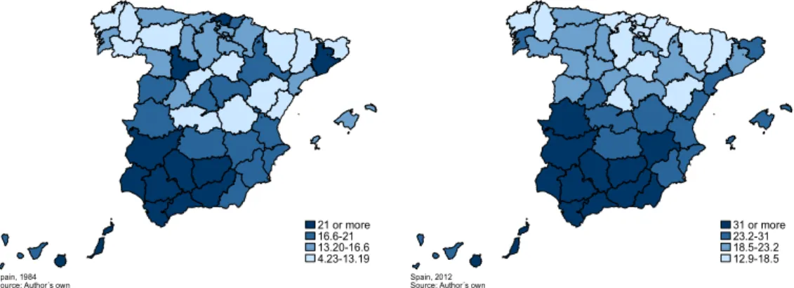
representation of the dynamics referred to in the introductory section, Figure 2 shows the provincial distribution of effective provincial unemployment in 1984 and 2012 through two maps of quartiles.
The data reveal the presence of substantial differences between effective provincial unemployment rates, which is reflected in the scale of the quartiles. A certain geographical pattern also emerges in the colour distribution. The highest rates are found in the southern most provinces and in the Canary Islands, whilst the provinces with the lowest rates are located in the north and northeast of the Iberian Peninsula. Finally, the similarity between the two maps in Figure 2 is clear evidence of the persistence in the provinces which
experience most (and fewest) problems of unemployment during the period analysed33.
30 Moran’s scatterplot diagrams (Anselin, 1995) provide a more comprehensive view of the existence of overall spatial dependence. 31 For a more detailed explanation of this kind of statistics, see Moreno and Vayá (2002).
32 Ceuta and Melilla have been excluded from the analysis due to their scant representativeness together with scarce availability of
some of the data used.
33The inverse situation can be found in the work of Galiani et al. (2005). In this research, the authors shows that the persistence of
21 or more 16.6-21 13.20-16.6 4.23-13.19 Spain, 1984
Source: Author´s own
31 or more 23.2-31 18.5-23.2 12.9-18.5 Spain, 2012
Source: Author´s own
Figure 2. Distribution of effective provincial unemployment rates
Table A1 of the Appendix provides a summary of the variables used in the work and of their calculation procedure. The central variable in this study is the effective provincial unemployment rate, and is the one which acts as the dependent variable and the one we seek to decompose. To achieve this decomposition, a series of independent variables will also be used which reflect the structural aspects and which explain their evolution over time. The first three explanatory variables, in Table A1 of the Appendix, refer to the industry composition of employment in each province. According to Elhorst (2003), industry composition proves a key factor when explaining differing unemployment rates at a territorial scale. The greater or lesser weight of certain industries is reflected in wage differences, skilled labour or competitiveness, and therefore emerges as a determinant
feature vis-à-vis accounting for the rate of unemployment from a territorial perspective34.
Other important variables for explaining the effective provincial unemployment rate are the female participation rate and the percentage represented by the 15 to 24 year old age group out of the total population. As regards the former, Elhorst (2003) consider that this variable might lead to dissimilar results when explaining the effective
unemployment rate35. The latter variable is purely demographic and tends to impact
positively on unemployment rates (Johnson and Kneebone, 1991; Murphy and Payne, 2003). One initial explanation for such a phenomenon might be that youngsters “seek worse employment” than those who are older. They possess fewer job-seeking skills and are less efficient than their older counterparts. As a result, the young tend to remain unemployed
for longer periods than those who are older36. Another explanation for this effect might be
that, in general, younger people possess less specific capital due to having little work
experience, which has a negative impact on their labour market matching37.
Finally, two variables have been included to reflect employed persons level of human capital. The first is the percentage of employed persons, out of the total number of employed persons, who have completed upper secondary education, and the second reflects the percentage of employed persons who have completed tertiary education out of the total
number of employed persons in each province38. Taking into account the work of Elhorst
(2003), variables measuring the level of human capital tend to have a negative impact on unemployment. It would seem logical to assume that those with higher educational attainment might develop skills that would enable them to adapt far more quickly and effectively to technological changes. This would make them more productive than those
34 In Summers et al. (1986) a more detailed explanation of the phenomenon may be found.
35 Lázaro et al. (2000), Azmat et al. (2006) and Bertola et al. (2007) provide explanations and hypotheses regarding high female
unemployment rates.
36 Maguire et al. (2013) provides a thorough explanation of this phenomenon.
37 See Eichhorst and Neder (2014) for a broader explanation of the problems related to the “school-work” transition in certain
European Mediterranean countries.
38 For a more detailed definition of educational variables, see
with lower educational attainment, as well as more desirable from the point of view of
being hired in addition to affording them greater work stability39.
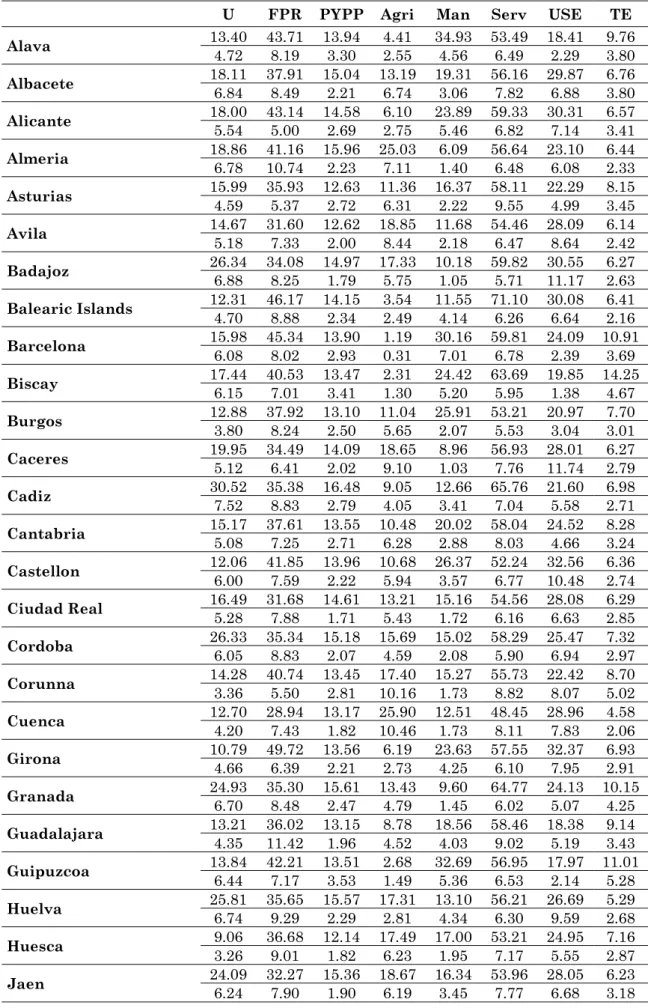
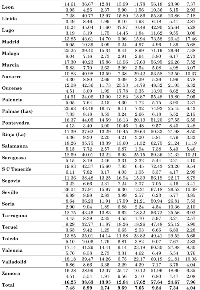
In order to provide more detailed information concerning the variables used, Appendix (Table A2) offers some descriptive statistics. The mean effective provincial unemployment rate for the period, as a central variable in our research, displays enormous variability, with the highest values being in Cadiz (30.52%) and Badajoz (26.34%), and the lowest in Lleida (7.28%) and Soria (8.64%). These interprovincial differences are also true of other variables. Female participation rates are extremely high in provinces such as Girona (49.72%) or the Balearic Islands (46.17%), whereas in Cuenca or Zamora they fail to reach 30%. As regards the weight of the youth population (15-24 years of age), variability amongst Spanish provinces is less notable. The provinces with the highest percentage of youngsters are Cadiz (16.48%) and Las Palmas (16.47%) whereas the lowest values are found in Lugo (11.6%) and Ourense (11.73%). As regards the variables reflecting industry composition, agriculture seems to be the industry with the greatest disparity at a provincial scale. Lugo is the province which stands out most, with 37.87% of persons employed in agriculture, followed by Cuenca with 25.9%. At the other end of the scale, agriculture accounts for less than 2% of all employment in the provinces of Madrid and Barcelona. In the manufacturing industry, the extremes are marked by Alava (34.93%) and Almeria (6.09%). Finally, the service industry presents the highest rates in Las Palmas (74.93%) and in Madrid (73.58%). In contrast, in provinces such as Lugo (42.9%) and Teruel (47.48%) it is far less important. The final variables are those reflecting the human capital of employed persons. In the case of those who have completed upper secondary education, the highest values are found in Castellon and Girona, with over 30%, whereas Guipuzcoa and Guadalajara are at the other end of the scale with values below 20%. Finally, the provinces displaying the highest percentage of employed persons with tertiary education qualifications are Madrid (17.46%) and Biscay (14.25%), in contrast to the lowest, which are Cuenca (4.58%) and Lugo (5.28%).
6.
Results
This section is divided into three blocks. The first shows the results of decomposing the unemployment rate. The second examines the existence of the spatial dependence of the effective unemployment rate and its components. Finally, the third block discusses the implications of the results to emerge.
6.1
Decomposing the effective unemployment rate
As already mentioned, decomposition of the effective unemployment rate was performed by applying the stochastic frontier technique. This frontier has been modelled following various specifications which increase the number of explanatory variables, and which are set out in equations (10), (11) and (12):
= + + + + 2001 + + + (10)
= + + + + + + 2001 + + + (11)
= + + + + + + + +
+ + 2001 + + + (12)
The most basic specification (equation 10) models the frontier with the variables reflecting the industry composition of labour and a dichotomous variable ( 2001) taking
the value 1 after the year 2001 and 0 otherwise40. The second specification (equation 11)
adds two new explanatory variables, female participation rate ( ) and the percentage of
the youth population in the province ( ). Finally, the most comprehensive specification
39 See López-Bazo and Motellón (2012) for a more comprehensive explanation of regional differences in the matter of human
capital, its impact on the labour market and on wages.
40 This dichotomous variable is introduced due to the fact that in 2001 a methodological change was implemented which affected
is represented by the equation 12. That equation includes four additional covariates, the
two for human capital ( and ) and the two components of a quadratic trend, the
lineal component of the trend ( ) and its quadratic component ( ). In addition, the models include fixed provincial effects to reflect unobservable heterogeneity ( ) at the provincial level.
Table A3 of the Appendix presents the results obtained for each of the specifications. Firstly, it should be pointed out that all the specifications display a stochastic cost frontier at a 1% level of significance41. If we commence by analysing the
industry variables, it can be seen how all the independent variables show positive and significant values, indicating that all the industries give rise to higher natural rates of unemployment in comparison with the industry of reference, which is the construction industry. It can also be seen that agriculture and manufacturing display very similar values and that the greatest effect on structural unemployment corresponds to the service industry. This result might be due to the weight which certain low-skilled jobs have in the service industry. Low-skilled workers are subject to higher turnover rates and are given
little training by firms42. This leads to a low-skilled labour force with low employability and
also triggers structural unemployment in the industry43.The two regressors added in
specification 2 also display a positive and significant sign which is also true of specification
3 (although the effect of the variable diminishes substantially when adding more
information to the model). The coefficient of the implies that the integration of women
into the labour market has helped to raise effective unemployment rates at an aggregate level, partly due to the fact their unemployment rates are almost higher than men’s. For its part, the coefficient related to the weight of the youth population bears out the hypothesis posited earlier that the young are less skilled at job-seeking than their more mature counterparts. It also reflects the difficulty said group has in finding work as a result of their possessing “less” specific capital. Finally, it highlights the importance of youth
unemployment when explaining the natural rate of unemployment44.
The results of the variables of human capital are consistent with the hypothesis put forward earlier and evidence a reducing effect on natural unemployment (specification 3). When the human capital of employed persons increases, the less is the likelihood of them becoming unemployed (Nickell and Bell, 1996). It can also be seen that the percentage of individuals with tertiary education qualifications are less likely to be unemployed than the other individuals who has upper secondary qualifications. The methodological changes implemented by the INE in 2001 had a negative and highly significant effect on all specifications (particularly in specifications 1 and 3). This indicates that the new method adopted by the INE contributed to the reduction of provincial unemployment. Finally, the trend included in specification 3 is also significant, with a sign which is negative in its lineal component and positive in the quadratic. Based on these estimations, the components of the effective unemployment rate detailed earlier are obtained and presented: the natural
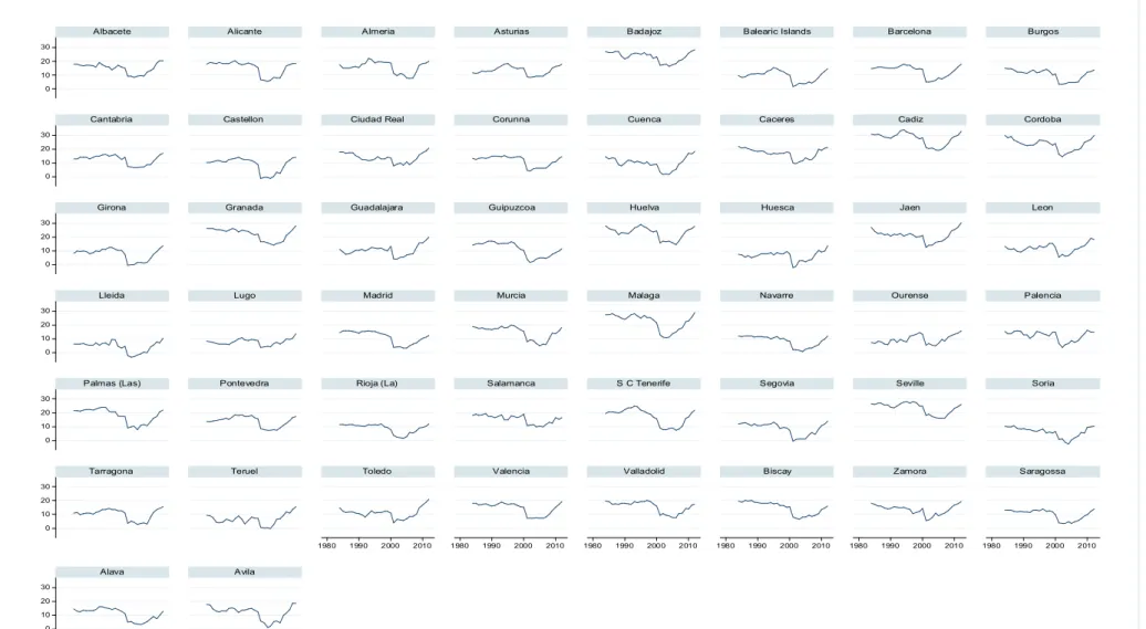
rate of unemployment and cyclical unemployment45. Figure 3 depicts the evolution of the
natural rate of unemployment for all Spanish provinces during the period 1984-201246. The
mean of that component for the whole period reaches a value of 13.47 although there is considerable interterritorial variability. The provinces displaying the highest mean value are Cadiz (27.58), Cordoba (23.43) and Badajoz (23.30) and those which behave best are Lleida (4.40), Soria (6.10) and Huesca (6.46)47.
41 The test of maximum likelihood rejects the notion that variance of the disturbance measuring inefficiency is zero. 42 A good example for the case of Spain might be certain jobs in the tourism industry.
43 Using a panel including 21 OECD countries, Oesch (2010) provides empirical evidence concerning which variables most impact
on unemployment among low-skilled workers.
44 The works of Dolado et al. (1999 and 2000) and Dolado et al. (2002) offer some explanations of the “deficient” functioning of the
labour market for the case of young people in Spain.
45 Some negative values have been obtained when estimating the natural rate of unemployment for certain provinces. Despite this,
said values account for only a very small part compared to the total number of estimations, and in all cases are below 2% of the total number of estimations obtained, bearing in mind the three specifications used.
46 Estimations were performed based on specification 3. Tests were carried out using specification 1 and specification 2 and the
results are very similar, with a correlation coefficient between the two specifications equal to 0.9635 and 0.9683, respectively. These results are available from the authors upon request.
0 10 20 30
0 10 20 30
0 10 20 30
0 10 20 30
0 10 20 30
0 10 20 30
0 10 20 30
1980 1990 2000 2010 1980 1990 2000 2010 1980 1990 2000 2010 1980 1990 2000 2010 1980 1990 2000 2010 1980 1990 2000 2010
1980 1990 2000 2010 1980 1990 2000 2010
Albacete Alicante Almeria Asturias Badajoz Balearic Islands Barcelona Burgos
Cantabria Castellon Ciudad Real Corunna Cuenca Caceres Cadiz Cordoba
Girona Granada Guadalajara Guipuzcoa Huelva Huesca Jaen Leon
Lleida Lugo Madrid Murcia Malaga Navarre Ourense Palencia
Palmas (Las) Pontevedra Rioja (La) Salamanca S C Tenerife Segovia Seville Soria
Tarragona Teruel Toledo Valencia Valladolid Biscay Zamora Saragossa
Alava Avila
Figure 3. Natural unemployment (
) by province (1984-2012)
0 5 10
0 5 10
0 5 10
0 5 10
0 5 10
0 5 10
0 5 10
1980 1990 2000 2010 1980 1990 2000 2010 1980 1990 2000 2010 1980 1990 2000 2010 1980 1990 2000 2010 1980 1990 2000 2010
1980 1990 2000 2010 1980 1990 2000 2010
Albacete Alicante Almeria Asturias Badajoz Balearic Islands Barcelona Burgos
Cantabria Castellon Ciudad Real Corunna Cuenca Caceres Cadiz Cordoba
Girona Granada Guadalajara Guipuzcoa Huelva Huesca Jaen Leon
Lleida Lugo Madrid Murcia Malaga Navarre Ourense Palencia
Palmas (Las) Pontevedra Rioja (La) Salamanca S C Tenerife Segovia Seville Soria
Tarragona Teruel Toledo Valencia Valladolid Biscay Zamora Saragossa
Alava Avila
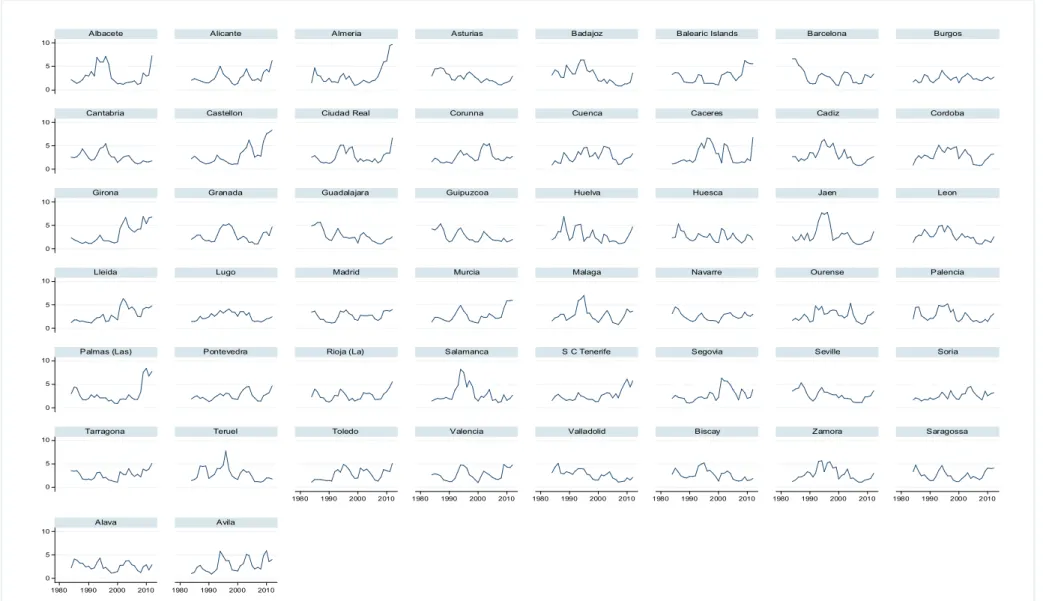
Figure 4. Cyclical unemployment ( ) by province (1984-2012)
Despite what was pointed out above, in order to gain a clearer understanding of how this element contributes to the effective unemployment rate, we should focus on relative values. The provinces whose natural component makes the greatest mean contribution to the effective unemployment rate are Cadiz (90.37%), Seville (89.58%) and Cordoba (88.95%). At the other end are Lleida (60.44%), Teruel (69.64%) and Soria (70.66%) which contribute less. Figure 3 also shows that the profile of the natural component is quite similar for all provinces. At the start of the period, it seems to remain fairly stable and at the end evidences a “U” shaped figure spanning the late 1990s and early part of the 21st century. As a result, there is a reduction in the natural rate of unemployment at the turn of the 21st century which, more or less, comes to an end with the onset of the economic crisis for the vast majority of provinces. Figure 4 shows the estimations of cyclical unemployment
( ) at a provincial scale48. In aggregate terms, this component shows a mean value equal
to 2.78, which represents approximately one fifth of the natural component.As occurred earlier, cyclical unemployment also displays enormous interprovincial diversity. Castellon (3.14), Girona (3.13) and Caceres (3.049) are the provinces with the highest mean values and Burgos (2.47), Soria (2.53) and Navarre (2.54) those with the lowest. Below the mean,
we also find Madrid, Guipuzcoa and Biscay49. Finally, certain similarities can also be found
in the evolution of all of them, with a final upturn coinciding with period linked to the Great Recession.
6.2
Spatial analysis of the effective unemployment rate and its
components
Having performed the decomposition, the next step involves analysing the spatial dependence of each component. In order to achieve this goal, it is necessary to start by defining the matrices. This work uses four different spatial matrices. The first considers the five closest neighbours to each province (knn=5)50. The second is a matrix of distances
which penalises spatial units that are furthest away from one another. The third is also a matrix of distances, but is based on the square of the inverse distance. Finally, the fourth is an administrative matrix which considers only provinces belonging to the same autonomous community to be neighbours.
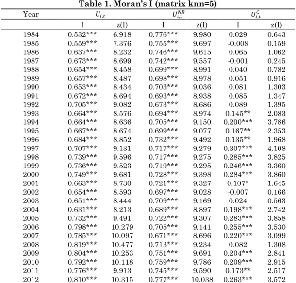
Table 1 shows the values corresponding to Moran’s I obtained from the spatial matrix which follows the criterion of the five closest neighbours51. The data evidence a
strong positive spatial dependence both in the effective provincial unemployment rates as well as in their natural component. The effective unemployment rate shows positive and significant values at a 1% level over the whole period. Even though the values are highly stable (keeping within a range between 0.5 and 0.81) they appear to increase over time, albeit only slightly. What was stated earlier indicates that effective unemployment rates resemble those of their neighbours as time passes. These results are borne out by the diagrams corresponding to section A) of Figure A1 of the Appendix. The results evidence a strong positive dependence which is reflected in the greater concentration of points in the first and third quadrant, particularly in the final year of the sample.
The results corresponding to the spatial analysis of the natural rate of unemployment are very similar to those presented for the effective unemployment rate. All the values of Moran’s I are positive and significant at a 1% level. In this case, the mean values are higher but display less variability (ranging between 0.67-0.77), evidencing greater stability of Moran’s I over the whole period. The Moran’s I scatterplot diagrams shown in section B) of figure A1 of the Appendix once again bear out all the results mentioned.
48 Estimations of cyclical unemployment have also been conducted using specification 1 and specification 2, with the results being
very similar. Estimations obtained using specifications 1 and 2 show a correlation coefficient equal to 0.8707 and 0.8887, respectively.
49 Detailed results are available to those interested upon request from the authors. 50 This type of spatial matrix is also used in Basile et al. (2009).
51 The results obtained for the remaining spatial matrices concur in pointing to the existence of spatial dependence for the effective
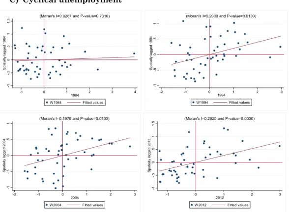
In all the years presented, a strong positive spatial dependence can be seen, with significant concentrations of points in the first and third quadrants. In the case of cyclical unemployment, the situation is not as clear. Moran’s I points to a positive spatial dependence, although this only occurs as of 1992 (and with the exception of 2002, 2003 and 2008). It can also be seen how the value of Moran’s I is lower than for the two previous cases and with values ranging between 0.1 and 0.3. This lower spatial dependence is also evident when observing the diagrams shown in section C) of Figure A1 of the Appendix. The points no longer display such a clear pattern and are distributed over the four quadrants.
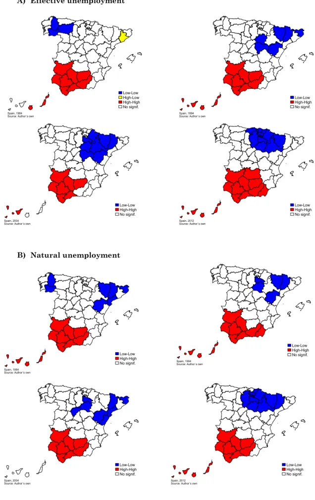
Having verified the existence of the positive spatial dependence of the unemployment rate and its components, the next step is to determine where the areas of “high” and “low” unemployment are situated and whether these persist over time. The three panels of Figure 5 show the results obtained using the local statistics of Moran’s I for
the unemployment rate and its components, and for the four years in the sample52. In panel
A), corresponding to the effective unemployment rate, two clearly defined geographical areas emerge. On the one hand, a cluster of “high” unemployment is located in the south of Spain, and which remains very stable over the four years studied, and which includes most of the provinces in Andalusia as well as Badajoz (in addition to Ciudad Real in 2012).
52 The results shown have been obtained using the 5knn matrix. Nevertheless, tests have been carried out using the remaining
spatial matrices and the conclusions are similar. The results of these tests are available to those interested upon request from the authors. Tests were also conducted after removing the islands. The values of the statistics did not alter substantially.
Table 1. Moran’s I (matrix knn=5)
Year , , ,
I z(I) I z(I) I z(I)
1984 0.532*** 6.918 0.776*** 9.980 0.029 0.643
1985 0.559*** 7.376 0.755*** 9.697 -0.008 0.159
1986 0.637*** 8.232 0.746*** 9.615 0.065 1.062
1987 0.673*** 8.699 0.742*** 9.557 -0.001 0.245
1988 0.654*** 8.458 0.699*** 8.991 0.040 0.782
1989 0.657*** 8.487 0.698*** 8.978 0.051 0.916
1990 0.653*** 8.434 0.703*** 9.036 0.081 1.303
1991 0.672*** 8.694 0.693*** 8.938 0.085 1.347
1992 0.705*** 9.082 0.673*** 8.686 0.089 1.395
1993 0.664*** 8.576 0.694*** 8.974 0.145** 2.083
1994 0.664*** 8.636 0.705*** 9.150 0.200*** 3.786
1995 0.667*** 8.674 0.699*** 9.077 0.167** 2.353
1996 0.684*** 8.852 0.732*** 9.492 0.135** 1.968
1997 0.707*** 9.131 0.717*** 9.279 0.307*** 4.108
1998 0.739*** 9.596 0.717*** 9.275 0.285*** 3.825
1999 0.736*** 9.523 0.719*** 9.295 0.246*** 3.360
2000 0.749*** 9.681 0.728*** 9.398 0.284*** 3.860
2001 0.663*** 8.730 0.721*** 9.327 0.107* 1.645
2002 0.654*** 8.593 0.697*** 9.028 -0.007 0.166
2003 0.651*** 8.444 0.709*** 9.169 0.024 0.563
2004 0.631*** 8.213 0.689*** 8.897 0.198*** 2.742
2005 0.732*** 9.491 0.722*** 9.307 0.283*** 3.858
2006 0.798*** 10.279 0.705*** 9.141 0.255*** 3.530
2007 0.785*** 10.097 0.671*** 8.696 0.220*** 3.099
2008 0.819*** 10.477 0.713*** 9.234 0.082 1.308
2009 0.804*** 10.253 0.751*** 9.691 0.204*** 2.841
2010 0.792*** 10.118 0.759*** 9.786 0.209*** 2.915
2011 0.776*** 9.913 0.745*** 9.590 0.173** 2.517
2012 0.810*** 10.315 0.777*** 10.038 0.263*** 3.572
Low-Low High-High No signif. Spain, 2004
Source: Author´s own
Figure 5. Local spatial dependence statistics (matrix knn=5)
A) Effective unemployment
B) Natural unemployment
Low-Low High-High No signif. Spain, 1994
Source: Author´s own
Low-Low High-High No signif. Spain, 2004
Source: Author´s own
Low-Low High-High No signif. Spain, 2012
Source: Author´s own
Low-Low High-High No signif. Spain, 1994
Source: Author´s own
Low-Low High-High No signif. Spain, 2012
Source: Author´s own Low-Low
High-Low High-High No signif. Spain, 1984
Source: Author´s own
Low-Low High-High No signif. Spain, 1984
C) Cyclical unemployment
On the other hand, there is an area of “low” unemployment in the north of Spain and which shifts over time towards the Basque Country, Navarre and Aragón, particularly after the second half of the 1990s. These results are also confirmed based on the local scatterplot diagrams presented in section A) of Figure A2 of the Appendix.
The same results obtained in panel A) for the effective unemployment rate also hold true in panel B) for the natural rate of unemployment. The cluster of very stable “high” unemployment found in the provinces of the southern half of the country is seen to remain. On the other hand, another cluster of “low” unemployment emerges in the south of the peninsula. That cluster changes over time and finally, in 2012, also ends up in the north-east of the peninsula. Once again, this result is consistent with what is shown in section B) in Figure A2 which appears in the Appendix. In the case of cyclical unemployment, the situation is far more erratic. There are clusters of “high” and “low” unemployment, but without any kind of territorial consistency in the years shown. This lack of any pattern is also apparent in section C) of Figure A2 with greater randomness in the distribution of the points.
6.3
Implications of the results
The previous results highlight the existence of two well-defined clusters of unemployment: one of “high” effective unemployment in the southern half of the peninsula, and another of “low” effective unemployment in the north-east of the peninsula. There is also evidence that these patterns are basically explained through the natural component of unemployment,
where “spatial persistence” is much more palpable than in cyclical component53.
Section 3.2 already set out some of the social and economic phenomena which might provide a tentative explanation for the existence of unemployment clusters. Bearing in mind that the spatial dependence of the unemployment rate is the result of the natural rate
53 Cracolici et al. (2007) define the notion of spatial persistence based on the situation which leads “adjacent provinces to display
unemployment rates that are similar over a spatial area and at different periods”.
Low-Low Low-High High-High No signif. Spain, 1994
Source: Author´s own
Low-Low High-High No signif. Spain, 2004
Source: Author´s own
Low-Low High-Low High-High No signif. Spain, 2012
Source: Author´s own Low-High
High-Low High-High No signif. Spain, 1984