HAAR SHIFTS, COMMUTATORS, AND HANKEL OPERATORS
MICHAEL LACEY
Abstract. Hankel operators lie at the junction of analytic and real-variables.
We will explore this junction, from the point of view of Haar shifts and com-mutators.
1. Haar Functions
We consider operators which satisfy invariance properties with respect to two well-known groups. The first group we take to thetranslationoperators
Tryf(x) :=f(x−y), y∈R. (1.1)
Note that formally, the adjoint operator is (Try)∗= Tr−y. The collection of
oper-ators{Try : y∈R} is a representation of the additive group (R,+).
It is an important, and very general principle that a linear operator L acting on some vector space of functions, which is assumed to commute with all translation operators, is in fact given as convolution, in general with respect to a measure or distribution, thus,
Lf(x) = Z
f(x−y)µ(dy).
For instance, with the identity operator,µ would be the Dirac pointmass at the origin.
The second group is the set ofdilations onLp, given by
Dil(λp)f(x) :=λ−1/pf(x/λ), 0< λ, p <∞. (1.2)
Here, we make the definition so thatkfkp=kDilλ(p)fkp. Thescale of the dilation
Dil(λp)is said to beλ, and these operators are a representation of the multiplicative group (R+,∗). The Haar measure of of this group isdy/y.
Underlying this subject are the delicate interplay between local averages and differences. Some of this interplay can be encoded into the combinatorics ofgrids, especially thedyadic grid,defined to beD:={2k(j, j+ 1) : j, k∈Z}.
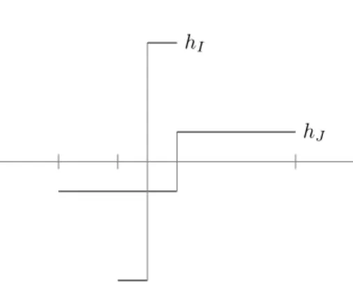
The Haar functions are a remarkable class of functions indexed by the dyadic gridD. Set
h(x) =−1(−1/2,0)+1(0,1/2),
2000 Mathematics Subject Classification. Primary: 47B35, 42B20 Secondary: 47B47,
hJ
hI
Figure 1. Two Haar functions.
a mean zero function supported on the interval (−1/2,1/2), taking two values, with L2 norm equal to one. Define theHaar function (associated to intervalI) to be
hI := Dil2IhI (1.3)
Dil(Ip):= Trc(I)Dil (p)
|I|, c(I) = center ofI. (1.4)
Here, we introduce the notion for theDilation associated with intervalI.
The Haar functions have profound properties, due to their connection to both analytical and probabilistic properties. An elemental property is that they form a basis forL2(R).
1.5. Theorem. The set of functions {1[0,1]} ∪ {hI : I ∈ D, I ⊂ [0,1]} form an orthonormal basis for L2([0,1]). The set of functions {h
I : I ∈ D} form an orthonormal basis forL2(R).
2. Paraproducts
Products, and certain kind of renormalized products are common objects. Let us explain the renormalized products in a very simple situation. We begin with the definition of aparaproduct, as a bilinear operator. Define
h0I =hI, h1I =|h0I|= Dil2I1[−1/2,1/2]. (2.1) The superscript0 indicates a mean-zero function, while the superscript1indicates a non-zero integral. Now define
Pǫ1,ǫ2,ǫ3(f1, f2) :=X I∈D
hf1, hǫ1 I i
p
|I| hf2, h
ǫ2
2 ih
ǫ3
I , ǫj∈ {0,1}. (2.2)
For the most part, we consider cases where there is one choice ofǫj which is equal
to one, but in considering fractional integrals, one considers examples where allǫj
important attribute is its signature. Indeed, in Proposition5.3, we will see that a paraproduct arises from a computation that, while not of the form above, is clearly an operator of signature (0,0,0). All the important prior work on commutators, see [1,2,6,7,9] can be interpreted in this notation. (The Lectures of M. Christ [5] are recommended as a guide to this literature.) For instance, in the notation of Coifman and Meyer [6,7], aPtdenotes a1, while aQtdenotes a0.
Why the name paraproduct? This is probably best explained by the identity
f1·f2= P1,0,0(f1, f2) + P0,0,1(f1, f2) + P0,1,0(f1, f2). (2.3) Thus, a product of two functions is a sum of three paraproducts. The three in-dividual paraproducts in many respects behave like products, for instance we will see that there is a H¨older Inequality. And, very importantly, in certain instances they arebetter than a product.
To verify (2.3), let us first make the self-evident observation that
1 |J|
Z
J
g(y)dy=hg, h 1
Ii
p |I| =
X
J:J)I
hg, hJihJ(I), (2.4)
wherehJ(I) is the (unique) valuehJ takes on I. In (2.3), expand bothf1 andf2
in the Haar basis,
f1·f2= (
X
I∈D
hf1, hIihI
) ·
( X
J∈D
hf2, hJihJ
) .
Split the resulting product into three sums, (1)I=J, (2)I(J (3)J (I. In the first case,
X
I,J:I=J
hf1, hIihf2, hJi(hI)2= P0,0,1(f1, f2).
In the second case, use (2.4).
X
I,J:I(J
hf1, hIihf2, hJihI·|I|1
Z
I
hJ(y)dy=
X
I
hf1, hIih
f2, h1
Ii
p |I| hI = P0,1,0(f1, f2).
And the third case is as in the second case, with the role off1 andf2 switched. A rudimentary property is that Paraproducts should respect H¨older’s inequality, a matter that we turn to next. This Theorem is due to Coifman and Meyer [6,7]. Also see [14,17,18].
2.5. Theorem. Suppose at most one of ǫ1, ǫ2, ǫ3 are equal to one. We have the inequalities
kPǫ1,ǫ2,ǫ3(f1, f2)k
3. Paraproducts and Carleson Embedding
We have indicated that Paraproducts are better than products in one way. These fundamental inequalities are the subject of this section. Let us define the notion of(dyadic) Bounded Mean Oscillation, BMO for short, by
kfkBMO= sup
J∈D
"
|J|−1X
I⊂J
hf, hRi2
#1/2
. (3.1)
3.2.Theorem. Suppose that at exactly one ofǫ2 andǫ3 are equal to1.
P0,ǫ2,ǫ3(f1,·)
p→p≃ kf1kBMO, 1< p <∞. (3.3) Indeed, we have
P0,1,0(f1,
·)p→p≃sup
J
P0,1,0(f1,
|J|−1/p1J)
p ≃ kf1kBMO. (3.4)
Here, we are treating the paraproduct as a linear operator on f2, and showing that the operator norm is characterized bykf1kBMO. Obviously,kfkBMO≤2kfk∞,
and again this a crucial point, there are unbounded functions with bounded mean oscillation, with the canonical example being lnx. Thus, these paraproducts are, in a specific sense, better than pointwise products of functions.
Proof. The case p = 2 is essential, and the only case considered in these notes. This particular case is frequently referred to asCarleson Embedding, a term that arises from the original application of the principal in the Corona Theorem.
Let us discuss the case of P0,1,0in detail. Note that the dual of the operator f2−→P0,1,0(f1, f2),
that is we keep f1 fixed, is the operator P0,0,1(f1,·), so it is enough to consider P0,1,0 in theL2 case.
One direction of the inequalities is as follows.
kP0,ǫ2,ǫ3(f1,·)k
2→2≥sup
J k
P0,ǫ2,ǫ3(f1, h1 J)kp
≥ kf1kBMO
as is easy to see from inspection. Thus, the BMO lower bound on the operator norm arises solely from testing against normalized indicator sets.
For the reverse inequality, we compare to the Maximal Function. Fixf1, f2, and let
Dk={I∈ D : |h
f2, hIi|
p
|I| ≃2
k}
LetD∗
k be the maximal intervals in Dk. TheL2-bound for the Maximal Function
gives us
X
k
22k X
I∗∈D∗
k
Then, forI∗∈ D∗
k we have
X
I∈Dk
I⊂I∗
hf1, hIi2khI
2 2= 2
2k X I∈Dk
I⊂I∗
hf1, hIi2
≤22kkf1k2BMO|I∗| And so we are done by (3.5).
4. Hilbert Transform
It is a useful Theorem, one that we shall return to later, that the set of operators L that are bounded fromL2(R) to itself, and commute with both translations and dilations have a special form. They are linear combinations of the Identity operator, and theHilbert transform. The latter operator, fundamental to this study, is given by
Hf(x) := p.v. Z
f(x−y) dy
y . (4.1)
Here, we take the integral in the principal value sense, as the kernel 1/y is not integrable. Taking advantage of the fact that the kernel is odd, one can see that the limit below
lim
ǫ→0 Z
ǫ<|y|<1/ǫ
f(x−y) dy
y (4.2)
exists for allx, providedf is a Schwartz function, say. Thus, H has an unambiguous definition on a dense class of functions, in allLp. We shall take (4.2) as our general
definition of principal value. The Hilbert transform is the canonical example of a
singular integral, that is one that has to be defined in some principal value sense. Observe that H, being convolution commutes with all translations. That is also commutes with all dilation operators follows from the observation that 1/y is a multiple of the multiplicative Haar measure. It can also be recovered in a remarkably transparent way from a simple to define operator based upon the Haar functions. Let us define
g=−1(−1/4,−1/4)+1(−1/4,1/4)−1(1/4,1/2) (4.3) = 2−1/2{h(
−1/2,0)+h(0,1/2)} (4.4) Hf =X
I∈D
hf, hIigI, (4.5)
where as before,gI = Dil(2)I g. It is clear thatHis a bounded operator onL2. What
is surprising is that that it can be used to recover the Hilbert transform exactly. The succinct motivation for this definition is that H(sin) = cos, so that ifhI is a
local sine, thengI is a local cosine.
4.6.Theorem (S. Petermichl [20]). There is a non-zero constant c so that
H =c lim
Y→∞
Z Y
0 Z 2
1
TryDil(2)λ HDil
(2) 1/λTr−y
dλ λ
dy
hI gI
Figure 2. A Haar functionhI and its dualgI.
As a Corollary, we have the estimatekHk2.1, asHis clearly bounded onL2. The operatorhis referred to as aHaar shift or as adyadic shift ([22]). Certain canonical singular integrals, like the Hilbert, Riesz and Beurling transform admit remarkably simple Haar shift variants, which fact can be used to prove a range of deep results. See for instance [8,21,23,24]. For applications of this notion to more general singular integrals, see [13, Section 4].
Proof. Consider the limit on the right in (4.7). This is seen to exist for eachx∈R for Schwartz functions f. While this is elementary, it might be useful for us to define the auxiliary operators
Tjf :=
X
I∈D |I|≤2j
hf, hjigj.
The individual terms of this series are rapidly convergent. As |I|becomes small, one uses the smoothness of the functionf. As|I|becomes large, one uses the fact thatf is integrable, and decays rapidly. Call the limitHfe .
Let us also note that the operator Tjis invariant under translations by an integer
multiple of 2j. Thus, the auxiliary operator
2−j Z 2j
0
Tr−tfTrt dt
will be translation invariant. ThusH is convolution with respect to a linear func-e tional on Schwartz functions, namely a distribution.
Concerning dilations, T is invariant under dilations by a power of 2. Now, dila-tions form a group under multiplication onR+, and this group has Haar measure dδ/δ so that the operator below will commute with all dilations.
Z 1 0
Dil21/δT Dil2δ
dδ δ
Thus,H commutes with all dilations.e
Therefore,H must be a linear combination of a Dirac delta function and convo-e lution with 1/y. (The function 1/|y|is also invariant under dilations, but the inner product with this function is not a linear functional on distributions.) Applying
e
1 3 4 1 2 (−3
4, 1 4)
(−12, 1 2)
γ0 γ−1
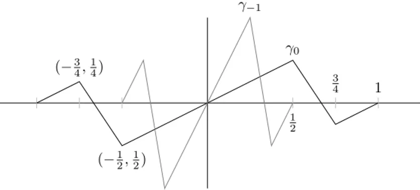
Figure 3. The graph ofγ0andγ−1.
must be a multiple of convolution with 1/y, and we only need to see that it is non zero multiple.
Let us set Gj to be the operator
Gjf :=
Z 2j 0
Trant
X
I∈D |I|=2j
hTran−tf, hIihI
dt 2j.
This operator translates with translation and hence is convolution. We can write Gjf = γj ∗f. By the dilation invariance of the Haar functions, we will have
γj = Dil12jγ0. A short calculation shows that γ0(y) =
Z 1 0
hI(y+t)hI(y)dt
This function is depicted in Figure3. Certainly the operatorPjGj is convolution
withPjγj(x). This kernel is odd and is strictly positive on [0,∞). This finishes
our proof.
5. Commutator Bound
We would like to explain a classical result on commutators.
5.1.Theorem. For a function b, and1< p <∞we have the equivalence
k[b,H]kp→p≃ kbkBMO, where this is the non-dyadicBMOgiven by
sup
I interval "
|I|−1 Z
I
f− |I|−1 Z
I
f(y)dy dx
We refer to this as a classical result, as it can be derived from the Nehari theorem, as we will explain below. The lower bound on the operator norm is found by applying the commutator to normalized indicators of integrals, and we suppress the proof.
Both bounds are very easy, if one appeals to the Nehari Theorem. See our com-ments on Nehari’s Theorem below. But, in many circumstances, different proofs admit different modifications, and so we present a ‘real-variable’ proof, deriving the upper bound from the Haar shift, and the Paraproduct bound in a transparent way.
Replacing the Hilbert transform by the Haar Shift, we prove
k[b,H]kp→p.kbkBMO (5.2)
The last norm is dyadic-BMO, which is strictly smaller than non-dyadic BMO. But Theorem 4.6 requires that we use all translates and dilates to recover the Hilbert transform, and so the non-dyadic BMO norm will be invariant under these translations and dilations.
The Proposition is that [b,H] can be explicitly computed as a sum of Paraprod-ucts which are bounded.
5.3.Proposition. We have
[b,H]f = P0,1,0(b,Hf)−H◦P0,1,0(b, f) (5.4) + P0,0,1(b,Hf)−H◦P0,0,1(b, f) (5.5)
+Pe0,0,0(b, f). (5.6)
In the last line,Pe0,0,0(b, f)is defined to be
e
P0,0,0(b, f) = X
I∈D
hb, h0
Ii
√ I hf, h
0
Ii(h0Ileft+h
0
Iright).
Each of the five terms on the right are Lp-bounded operators on f, provided
b ∈ BMO, so that the upper bound on the commutator norm in Theorem 5.1
follows as an easy corollary. The paraproduct in (5.6) does not hew to our narrow definition of a Paraproduct, but it is degenerate in that it is of signature (0,0,0), and thus even easier to control than the other terms.
Proof. Now, [b,H]f =bHf −H(b·f). Apply (2.3) to both of these products. We see that
[b,H]f = X
~ǫ=(1,0,0),(0,1,0),(0,0,1)
P~ǫ(b,Hf)−HP~ǫ(b, f).
The choices of~ǫ= (0,1,0),(0,0,1) lead to the first four terms on the right in (5.4). The terms that require more care are the difference of the two terms in which a 1 falls on ab. In fact, we will have
To analyze this difference quickly, let us write
hHf, hIi= sgn(I)hf, hPar(I)i
where Par(I) is the ‘parent’ ofI, and sgn(I) = 1 ifIis the left-half of Par(I), and is otherwise−1. This definition follows immediately from the definition of gI in
(4.3). Now observe that
hP~ǫ(b,Hf), h0Ii=hHf,P ~ǫ
(b, h0I)i
= hb, h 1
Ii
p
|I| · hHf, h 0
Ii
=hf, h0Par(I),isgn(I)h
b, h1
Ii
p |I| And on the other hand, we have
hHP1,0,0(b, f), hIi=
hb, h1 Par(I)i p
|Par(I)| sgn(I)hf, h 0 Par(I)i
Comparing these two terms, we see that we should examine the term that falls on b. But a calculation shows that
√
2h1I −h1Par(I)=−sgn(I)h 0 Par(I). Thus, we see that this difference is of the claimed form.
6. The Nehari Theorem
We define Hankel operators on the real line. On L2(R), we have the Fourier transform
b f(ξ) =
Z
f(x) e−iξx dx .
Define the orthogonal projections onto positive and negative frequencies
P±f(x)
def =
Z
R±
b
f(ξ) eiξx dx .
Define Hardy spacesH2(R) def= P+L2(R). Functionsf ∈H2(R) admit an analytic extension to the upper half planeC+. As in the case of the disk, it is convenient to refer to functions inH2(R) asanalytic.
A Hankel operator with symbol b is then a linear operator from H2(C+) to H2
+(C+) given by Hbϕ def= P+Mbϕ. This only depends on the analytic part ofb.
It is typical to include the notationC+ to emphasize the connection with analytic function theory, and the relevant domain upon which one is working. Below, we will suppress this notation.
6.1. Nehari’s Theorem ([19]). The Hankel operator Hb is bounded from H2 to
H2 iff there is a bounded functionβ with P+b=P+β. Moreover, kHbk= inf
β: P+β=P+b
kβk∞ (6.2)
Less exactly, we have kHbk ≃ kP+bkBMO, where we can take the last norm to be
non-dyadic BMO.
This Theorem was proved in 1954, appealing to the following classical fact.
6.3.Proposition. Each functionf ∈H1 is a product of functionsf1, f2∈H2. In particular, f1 andf2 can be chosen so that
kfkH1=kf1kH2kf2kH2
Given a bounded Hankel operator Hb, we want to show that we can construct a
bounded functionβ so that the analytic part ofbandβ agree.
This proof is the one found by Nehari [19]. We begin with a basic computation of the norm of the Hankel operator Hb:
kHbk= sup kϕkH2=1
sup
kψkH2=1
Z
Hbψ·ϕ dx
= sup
kϕkH2=1
sup
kψkH2=1
Z
P+Mbψ·ϕ dx
= sup
kϕkH2=1
sup
kψkH2=1
Z
(P+b)ψ·ϕ dx
= sup
kϕkH2=1
sup
kψkH2=1
h(P+b), ψ·ϕi
(6.4)
But, the H1 = H2 ·H2, as we recalled in Proposition 6.3. We read from the equality above that the analytic part ofb defines a bounded linear functional on H1a subspace ofL1.
The Hahn Banach Theorem applies, giving us an extension of this linear func-tional to all ofL1, with the same norm. But a linear function onL1is a bounded function, hence we have constructed a bounded functionβ with the same analytic part asb.
The calculation (6.4) is more general than what we have indicated here, a point that we return to below.
Let us remark that theHpvariant of Nehari’s Theorem holds. On the one hand,
one hasHp·Hp′ ⊂H1, so that the upper bound on the normkH
bkHp→Hp follows. On the other, Proposition 6.3 extends to the Hp-Hp′
factorization, whence the same argument for the lower bound can be used.
There is a close connection between commutators [b,H] and Hankel operators. Indeed, we have
The two terms on the right can be recognized as two Hankel operators with orthog-onal domains and ranges. Indeed, keep in mind the elementary identities P2+= P+, P+P− = 0, H = I−2 P−, and [b,I] = 0. Then, observe
P+[b,H] P−=−2 P+[b,P−] P−
=−P+bP2−+ P+P−bP−=−P+bP−
P−[b,H] P−= P−[b,P+] P−= 0
There are two additional calculations, which are dual to these and we omit them.
7. Further Applications
The author came to the Haar shift approach to the commutator from studies of Multi-Parameter Nehari Theorem [10,16]. The paper [15] surveys these two papers. This subject requires an understanding of the structure of product BMO that goes beyond the foundational papers of S.-Y. Chang and R. Fefferman [3,4] on the subject.
In particular, as in Nehari’s Theorem, the upper bound on the Hankel operator is trivial, as one direction of the factorization result is trivial: H2·H2⊂H1. The lower bound is however very far from trivial, as factorization is known to fail in product Hardy spaces. Indeed, Nehari’s theorem is equivalent to so-called weak
factorization, one of the points of interest in the Theorem. See [10,15,16] for a discussion of this important obstruction to the proof, and relevant references.
There are different critical ingredients needed for the proof of the lower bound. One of them is a very precise quantitative understanding of the proof of the upper bound. It is at this point that the techniques indicated in this paper are essential. The fundamentals of the multi-parameter Paraproduct theory were developed by Journ´e [11,12]. The subject has been revisited recently to develop novel Leibnitz rules by Muscalu, Pipher, Tao and Thiele [17,18]. Also see [14].
An influential extension of the classical Nehari Theorem to a real-variable setting was found by Coifman, Rochberg and Weiss [9]: Real-valued BMO onRn can be characterized in terms of commutators with Riesz Transforms. The real-variable setting implies a complete loss of analyticity, making neither bound easy. Recently, the author, with Pipher, Petermichl and Wick, have proved the multi-parameter extension of the this result [13]. This paper includes in it a quantification of the Proposition5.3to the higher dimensional setting, for (smooth) Calder´on Zygmund operators T: [b, T] is a sum of bounded paraproducts, a crucial Lemma in that paper. See [13, Proposition 5.11]. Such an observation is not new, as it can be found in e. g. [1] for instance. Still the presentation of Proposition5.3in this paper is as simple as any the author is aware of in the literature.
References
[1] Pascal Auscher and Michael E. Taylor, Paradifferential operators and commutator esti-mates, Comm. Partial Differential Equations20(1995), no. 9-10, 1743–1775. MR1349230
[2] Jean-Michel Bony,Calcul symbolique et propagation des singularit´es pour les ´equations aux d´eriv´ees partielles non lin´eaires, Ann. Sci. ´Ecole Norm. Sup. (4) 14(1981), no. 2, 209–246
(French). MR631751 (84h:35177)↑3
[3] Sun-Yung A. Chang and Robert Fefferman,Some recent developments in Fourier analysis and Hp-theory on product domains, Bull. Amer. Math. Soc. (N.S.)12(1985), no. 1, 1–43.
MR86g:42038↑11
[4] ,A continuous version of duality ofH1 with BMO on the bidisc, Ann. of Math. (2)
112(1980), no. 1, 179–201. MR82a:32009↑11
[5] Michael Christ,Lectures on singular integral operators, CBMS Regional Conference Series in Mathematics, vol. 77, Published for the Conference Board of the Mathematical Sciences, Washington, DC, 1990. MR1104656 (92f:42021)↑3
[6] R. Coifman and Y. Meyer, Commutateurs d’int´egrales singuli`eres et op´erateurs multi-lin´eaires, Ann. Inst. Fourier (Grenoble)28(1978), no. 3, xi, 177–202 (French, with English
summary). MR511821 (80a:47076) ↑3
[7] Ronald R. Coifman and Yves Meyer,Au del`a des op´erateurs pseudo-diff´erentiels, Ast´erisque, vol. 57, Soci´et´e Math´ematique de France, Paris, 1978 (French). MR518170 (81b:47061)↑3
[8] Oliver Dragiˇcevi´c and Alexander Volberg,Bellman function, Littlewood-Paley estimates and asymptotics for the Ahlfors-Beurling operator inLp(C), Indiana Univ. Math. J.54(2005),
no. 4, 971–995. MR2164413 (2006i:30025)↑6
[9] R. R. Coifman, R. Rochberg, and Guido Weiss,Factorization theorems for Hardy spaces in several variables, Ann. of Math. (2)103(1976), no. 3, 611–635. MR54#843↑3,11
[10] Sarah H. Ferguson and Michael T. Lacey,A characterization of product BMO by commuta-tors, Acta Math.189(2002), no. 2, 143–160.1 961 195↑11
[11] Jean-Lin Journ´e,Calder´on-Zygmund operators on product spaces, Rev. Mat. Iberoamericana
1(1985), no. 3, 55–91. MR88d:42028↑11
[12] ,Two problems of Calder´on-Zygmund theory on product-spaces, Ann. Inst. Fourier (Grenoble)38(1988), no. 1, 111–132. MR949001 (90b:42031)↑11
[13] Michael T. Lacey, Jill C. Pipher, Stefanie Petermichl, and Brett D. Wick, Multipa-rameter Riesz Commutators, Amer. J. Math. 131 (2009), no. 3, 731–769, available at
arxiv:0704.3720v1. MR2530853↑6,11
[14] Michael T Lacey and Jason Metcalfe,Paraproducts in One and Several Parameters, Forum Math.19(2007), no. 2, 325–351. MR2313844↑3,11
[15] Michael T. Lacey,Lectures on Nehari’s Theorem on the Polydisk, Topics in Harmonic Anal-ysis and Ergodic Theory, 2007, pp. 185-214, available atarXiv:math.CA/060127d.↑11
[16] Michael T Lacey and Erin Terwilleger, Hankel Operators in Several Complex Vari-ables and Product BMO, Houston J. Math. 35 (2009), no. 1, 159–183, available at arXiv:math.CA/0310348. MR2491875↑11
[17] Camil Mucalu, Jill Pipher, Terrance Tao, and Christoph Thiele,Bi-parameter paraproducts, Acta Math.193(2004), no. 2, 269–296. MR2134868 (2005m:42028)↑3,11
[18] , Multi-parameter paraproducts, Rev. Mat. Iberoam. 22 (2006), no. 3, 963–976.
MR2320408 (2008b:42037)↑3,11
[19] Zeev Nehari,On bounded bilinear forms, Ann. of Math. (2)65(1957), 153–162. MR18,633f
↑10
[20] Stefanie Petermichl, Dyadic shifts and a logarithmic estimate for Hankel operators with matrix symbol, C. R. Acad. Sci. Paris S´er. I Math.330(2000), no. 6, 455–460 (English, with
English and French summaries). MR1756958 (2000m:42016)↑5
[21] Stefanie Petermichl and Alexander Volberg,Heating of the Ahlfors-Beurling operator: weakly quasiregular maps on the plane are quasiregular, Duke Math. J.112(2002), no. 2, 281–305. MR1894362 (2003d:42025)↑6
[23] S. Petermichl,The sharp bound for the Hilbert transform on weighted Lebesgue spaces in terms of the classical Ap characteristic, Amer. J. Math. 129 (2007), no. 5, 1355–1375. MR2354322↑6
[24] Stefanie Petermichl,The sharp weighted bound for the Riesz transforms, Proc. Amer. Math. Soc.136(2008), no. 4, 1237–1249. MR2367098↑6
Michael Lacey
School of Mathematics Georgia Institute of Technology Atlanta GA 30332, USA lacey@math.gatech.edu