Finite dimensional Hopf algebras over the Kac–Paljutkin algebra $H 8$

https://doi.org/10.33044/revuma.v60n1a17

FINITE-DIMENSIONAL HOPF ALGEBRAS OVER THE KAC–PALJUTKIN ALGEBRA H8

YUXING SHI

Abstract. LetH8be the Kac–Paljutkin algebra [Trudy Moskov. Mat. Obˇsˇc. 15 (1966), 224–261], which is the neither commutative nor cocommutative semisimple eight dimensional Hopf algebra. All simple Yetter–Drinfel’d mod-ules over H8 are given, and finite-dimensional Nichols algebras overH8 are determined completely. It turns out that they are all of diagonal type. In fact, they are of Cartan typesA1,A2,A2×A2,A1×· · ·×A1, andA1×· · ·×A1×A2, respectively. By the way, we calculate Gelfand–Kirillov dimensions for some Nichols algebras. As an application, we complete the classification of the finite-dimensional Hopf algebras overH8according to the lifting method.

1. _Introduction

Let K be an algebraically closed field of characteristic zero. The question of

classification of all Hopf algebras over Kof a given dimension up to isomorphism

was posed by Kaplansky in 1975 [40]. Some progress has been made but, in general, it is a difficult question for lack of standard methods. One breakthrough is the so-called lifting method introduced by Andruskiewitsch and Schneider in 1998 [3], under the assumption that the coradical is a Hopf subalgebra.

We describe the procedure for the lifting method briefly. LetHbe a Hopf algebra whose coradicalH0 is a Hopf subalgebra. The associated graded Hopf algebra of

H is isomorphic to R#H0, where R = ⊕n∈N0R(n) is a braided Hopf algebra in the categoryH0

H0YDof Yetter–Drinfel’d modules overH0, # stands for the Radford

biproduct or bosonization of R with H0. As explained in [14], to classify finite-dimensional Hopf algebrasH whose coradical is isomorphic toH0we have to deal with the following questions:

(a) Determine all Yetter–Drinfel’d modules V over H0 such that the Nichols

algebraB(V) has finite dimension; find an efficient set of relations forB(V).

2010Mathematics Subject Classification. Primary 17B37, 81R50; Secondary 17B35.

Key words and phrases. Nichols algebra; Hopf algebra; Gelfand–Kirillov dimension; Kac– Paljutkin algebra.

(b) IfR=⊕n∈N0R(n) is a finite-dimensional Hopf algebra in

H0

H0YDwithV =

R(1), decide ifR'B(V). HereV =R(1) is a braided vector space called theinfinitesimal braiding.

(c) GivenV as in (a), classify allH such that grH 'B(V)#H0 (lifting). AliftingofV ∈H

HYDis a Hopf algebraLsuch that grL=B(V)#H, where grL

is the graded Hopf algebra associated to the coradical filtration. In other words [16, Proposition 2.4],Lis a lifting ofV iff there is an epimorphism of Hopf algebras

φ:T(V)BT(V)#H →Lsuch thatφ|H = idH and

φ|H⊕V#H:H⊕V#H →L1is an isomorphism of Hopf bimodules. (1.1)

Suchφis called alifting map. If emphasis onH is needed, then we say thatLis a lifting ofV overH.

The lifting method was extensively used in the classification of finite-dimensional pointed Hopf algebras such as [15], [12], [25], [23], [2], [1], [9], [8] and so on. It is also effective to study finite-dimensional copointed Hopf algebras ([16], [27], [22]). We note that there are very few classification results on finite-dimensional Hopf algebras whose coradical is neither a group algebra nor the dual of a group algebra, some exceptions being [19], [26], [11]. It should be mentioned that [11] constructed Hopf algebras with the Chevalley property over a semisimple Hopf algebraH that is Morita-equivalent to a group algebra _KG (in the sense of H_HYD ' KG

KGYD as

braided tensor categories). It doesn’t cover our case sinceH8can be obtained from a group algebra by a 2-pseudo-cocycle twist but not by a 2-cocycle twist [45].

Here we would like to initiate a project for the study of Hopf algebras whose coradicals are low-dimensional neither commutative nor cocommutative semisim-ple Hopf algebras by running procedures of the lifting method. One important step is to study the Nichols algebras over those low-dimensional semisimple Hopf algebras. Nichols algebras were studied first by Nichols [44]. These are connected graded braided Hopf algebras [4] generated by primitive elements, and all primi-tive elements are of degree one. In the past decades, the study of Nichols algebras was mainly focused on categories of Yetter–Drinfel’d modules over group algebras. Under the assumption that the base field has characteristic 0, the classification of finite-dimensional Nichols algebras over abelian groups was completely solved in [30, 31] by using Lie theoretic structures, and the result of the classification played an important role later in the significant work [15]. The problem of classifying finite-dimensional Nichols algebras over non-abelian groups is difficult in general for lack of systematic method; for related works please refer to [12], [24], [29], [32], [33], [36], [35], etc.

In this paper, we mainly focus on the Kac–Paljutkin algebraH8. The structure of our paper is as follows. In Section 2, we recall the fundamental notions related to Yetter–Drinfel’d modules, Nichols algebras and Gelfand–Kirillov dimension. In section 3, we construct all the simple left Yetter–Drinfel’d modules overH8

accord-ing to Radford’s method. In section 4, we get all the possible finite-dimensional Nichols algebras from Yetter–Drinfel’d modules over H8. It turns out that they

are of Cartan typesA1,A2,A2×A2,A1× · · · ×A1, andA1× · · · ×A1×A2. Here

Theorem A.LetM ∈H8

H8YD. Then the Nichols algebraB(M)is finite-dimensional

iffM is isomorphic to one of the following Yetter–Drinfel’d modules:

(1) Ω1(n1, n2, n3, n4)BL4j=1Mhbj, gji

⊕nj _withP4

j=1nj ≥1,(b1, g1) = (i, x),

(b2, g2) = (−i, x), (b3, g3) = (i, y) and (b4, g4) = (−i, y), the infinitesimal braiding is of typeA1× · · · ×A1

| {z }

n1+n2+n3+n4

.

(2) Ω2(n1, n2) B Mhi, xi⊕n1 _{⊕Mh−i, xi}⊕n2 _{⊕Mh(xy, x)i, n}

1+n2 ≥ 0, the infinitesimal braiding is of typeA1× · · · ×A1

| {z }

n1+n2

×A2.

(3) Ω3(n1, n2) B Mhi, yi⊕n1 _{⊕Mh−i, yi}⊕n2 _{⊕Mh(y, xy)i, n1+n2 ≥ 0, the}

infinitesimal braiding is of typeA1× · · · ×A1

| {z }

n1+n2

×A2.

(4) Ω4(n1, n2)BMhi, xi⊕n1⊕_Mh_i, yi⊕n2⊕_W1,−1_,n

1+n2≥0, the infinites-imal braiding is of typeA1× · · · ×A1

| {z }

n1+n2

×A2.

(5) Ω5(n1, n2) B Mh−i, xi⊕n1 _{⊕Mh−i, yi}⊕n2 _⊕W−1,−1_{, n1 +n2 ≥ 0, the}

infinitesimal braiding is of typeA1× · · · ×A1

| {z }

n1+n2

×A2.

(6) Ω6BMh(xy, x)i⊕Mh(y, xy)i, the infinitesimal braiding is of typeA2×A2.

(7) Ω7BW1,−1⊕W−1,−1, the infinitesimal braiding is of typeA2×A2. Remark 1.1. We point out which of the Yetter–Drinfel’d modules have a prin-cipal realization and which not, since the liftings are known when there is a principal realization and not otherwise [5, Subsection 2.2]. Let (h) and (δh) be

dual bases of H8 and H8∗, and b ∈ {±1,±i}. Define χb B δ1+δxy +b2(δx+ δy) + b(δz +δzxy) + b3_{(δzx +δzy) ∈ Alg(H8,}

K), then (g, χb) is a YD-pair [7]

iff _Kχb

g ' Mhb, gi is a one-dimensional Yetter–Drinfel’d module. Mh(g1, g2)i for

(g1, g2)∈ {(xy, x),(y, xy)} andWb1,−1 _{forb1=±1 don’t have a principal} realiza-tion. So only Ω1(n1, n2, n3, n4) has a principal realization.

In section 5, according to the lifting method, we give a classification for finite-dimensional Hopf algebras overH8. Here is the second main result.

Theorem B. Let H be a finite-dimensional Hopf algebra over H8 such that its infinitesimal braiding is inH8

H8YD. ThenH is isomorphic to either of: (1) A1(n1, n2, n3, n4;I1), see Definition 5.4;

(2) B[Ω2(n1, n2)]#H8, see Proposition 5.10;

(3) A4(n1, n2;I4), see Definition 5.18;

(4) A6(λ), see Definition 5.11;

(5) A7(I7), see Definition 5.15.

A1(n1, n2, n3, n4;I1) comprises two 16-dimensional nonisomorphic nonpointed

self-dual Hopf algebras with coradicalH8described in [19] as special cases. Except

2. _{Preliminaries}

2.1. Conventions. LetH be a Hopf algebra over_K, with antipodeS. We will use Sweedler’s notation ∆(h) = h(1)⊗h(2) for the comultiplication ([43]). LetHHYD

be the category of left Yetter–Drinfel’d modules over H. A left Yetter–Drinfel’d moduleMoverH is a leftH-module (M,·) and a leftH-comodule (M, ρ) satisfying

ρ(h·m) =h(1)m(−1)S(h(3))⊗h(2)·m(0), ∀m∈M, h∈H, (2.1)

where ρ(m) =m(−1)⊗m(0). The categoryHHYDis a braided monoidal category.

The braidingc∈End_K(M⊗M) ofM is defined byc(v⊗w) =v(−1)·w⊗v(0), and

the inverse braiding is defined byc−1_{(v⊗w) =w}

(0)⊗ S−1(w(−1))·v

.

Definition 2.1 ([14, Definition 2.1]). Let H be a Hopf algebra and V ∈ H HYD.

A braided N-graded Hopf algebra R =Ln≥0R(n) ∈ H

HYD is called the Nichols algebra ofV if

(i) _K'R(0),V 'R(1)∈H HYD.

(ii) R(1) =P(R) ={r∈R|∆R(r) =r⊗1 + 1⊗r}.

(iii) Ris generated as an algebra by R(1). In this case,Ris denoted byB(V) =L

n≥0B n_(V).

Remark 2.2. The Nichols algebraB(V) is completely determined by the braiding. More precisely, as proved in [49] and noted in [14],

B(V) = K⊕V ⊕

∞

M

n=2

V⊗n/kerSn =T(V)/kerS,

whereSn,1∈EndK V

⊗(n+1)

,Sn ∈EndK(V

⊗n_),

Sn,1Bid +cn+cncn−1+· · ·+cncn−1· · ·c1= id +cnSn−1,1,

S1Bid, S2Bid +c, SnB(Sn−1⊗id)Sn−1,1.

Lemma 2.3 ([28, Theorem 2.2], [6, Remark 1.4]). Let M1, M2 ∈ H

HYD be both finite-dimensional and assume cM1,M2cM2,M1 = idM2⊗M1. Then B(M1⊕M2) ' B(M1)⊗B(M2)as graded vector spaces andGKdimB(M1⊕M2) = GKdimB(M1)+

GKdimB(M2).

Proposition 2.4([46, Radford biproduct]).LetHbe a Hopf algebra andA∈H HYD be a braided Hopf algebra. Then A#H is a Hopf algebra with

∆(a#h) =X a(1)#(a(2))(−1)h(1)

⊗

(a(2))(0)#h(2)

, (2.2)

S(a#h) =X 1#SH(h)SH(a(−1))

SA(a(0))#1

, (2.3)

(a#h)(a0#h0) =Xa(h(1)·a0)#h(2)h0, a, a0∈A, h, h0∈H. (2.4)

The mapι:H →A#H given byι(h) = 1#hfor allh∈H is an injective Hopf algebra map, and the mapπ:A#H →H given byπ(a#h) =εA(a)hfor alla∈A, h∈H is a surjective Hopf algebra map such thatπ◦ι= idH. Moreover, it holds

Conversely, let B be a Hopf algebra with bijective antipode and π:B → H a Hopf algebra epimorphism admitting a Hopf algebra sectionι:H →B such that

π◦ι= idH. ThenA=Bcoπ is a braided Hopf algebra inHHYD andB'A#H as

Hopf algebras.

2.2. GK-dimension. Let A be a finitely generated algebra over a field K, and

assume a1, . . . , am generate A. Set V to be the span of a1, . . . , am, and denote Vn _{the span of all monomials in the a}

i’s of lengthn. Asai’s generate A one has A=S∞

k=0Ak, whereAk =K+V +V2+· · ·+Vk. The function dV(n) = dimAn

is the growth function of A. The Gelfand–Kirillov dimension of a _K-algebra A

is GKdimA = lim log_ndV(n). GKdimA does not depend on the choice of V.

Suppose that GKdimA <∞. We say that a finite-dimensional subspaceV ⊆Ais

GK-deterministicif

GKdimA= lim

n→∞logndim

X

0≤j≤n Vj.

Clearly, if V is a GK-deterministic subspace of A, then any finite-dimensional subspace ofA containing V is GK-deterministic. Let A and B be two algebras. Then

GKdim(A⊗B)≤GKdimA+ GKdimB,

but the equality does not hold in general. However, it does hold when A or B

has a GK-deterministic subspace, see [41, Proposition 3.11]. The Gelfand–Kirillov dimension is a useful tool in ring theory and Hopf algebraic theories. We shall not discuss in detail its importance but we refer the reader to [41] as a basic reference and [51, 50, 18, 6] for additional information related with Hopf algebras.

3. Simple Yetter–Drinfel’d modules ofH8

Recall that the neither commutative nor cocommutative semisimple 8-dimen-sional Hopf algebra H8 in [42] is constructed as an extension of K[C2×C2] by K[C2]. A basis forH8is given by{1, x, y, xy=yx, z, xz, yz, xyz}with the relations

x2=y2= 1, z2=1

2(1 +x+y−xy), xy=yx, zx=yz, zy=xz. The coalgebra structure and the antipode are defined by

∆(x) =x⊗x, ∆(y) =y⊗y, ε(x) =ε(y) = 1, S(x) =x, S(y) =y,

∆(z) = 1

2(1⊗1 + 1⊗x+y⊗1−y⊗x)(z⊗z), ε(z) = 1, S(z) =z. The automorphism group ofH8is the Klein four-group [48]. These automorphisms are given in Table 1; they are going to be used in Corollary 5.3.

Denote a set of central orthogonal idempotents of H8 as

e1=1

8(1 +x)(1 +y)(1 +z), e2= 1

8(1 +x)(1 +y)(1−z),

e3= 1

8(1−x)(1−y)(1 + iz), e4= 1

1 x y z

τ1= id 1 x y z

τ2 1 x y xyz

τ3 1 y x 1₂(z+xz+yz−xyz)

τ4 1 y x 1₂(−z+xz+yz+xyz)

Table 1. Hopf algebra automorphisms ofH8.

e5=

1−xy

2 , ejek =δjk, j, k= 1, . . . ,5; i =

√ −1;

and denote idempotentse0₅=1₄(1−xy)(1 +z),e00₅ =1₄(1−xy)(1−z). Then

H8=H8e1⊕H8e2⊕H8e3⊕H8e4⊕H8e5

=H8e1⊕H8e2⊕H8e3⊕H8e4⊕(H8e50 +H8e005),

whereH8e05'H8e005 as leftH8-modules, via e057→xe005,xe057→e005.

Definition 3.1. Denote V1(b) B K{v | x·v = b2v, y·v = b2v, z·v = bv, b ∈ {±1,±i}}, wherev is a vector. LetV2 'H8e05 as left H8-modules; the actions of

the generators are given by

x7→

0 1

1 0

, y7→

0 −1

−1 0

, z7→

1 0

0 −1

.

Proposition 3.2. All simple left modules of H8 are classified by V1(b), V2, b ∈ {±1,±i}.

Remark 3.3. The result was also obtained in [20] under a different basis (thanks to referee for reminding us about this fact).

In the remaining part of the article,V1(b) and V2 always mean simple leftH8 -modules.

Lemma 3.4([47, Proposition 2]). Let H be a bialgebra over a fieldKand suppose S is the antipode of H.

(1) If L ∈HM, thenL⊗H ∈ HYDH; the module and comodule actions are given by

h·(`⊗a) =h(2)·`⊗h(3)aS−1(h(1)), ρ(`⊗h) = (`⊗h(1))⊗h(2), ∀h, a∈H, `∈L. Let M ∈HYDH.

(2) Suppose thatL∈HMandp:M −→L is a map of leftH-modules. Then the linear map f : M −→ L⊗H defined by f(m) =p(m(0))⊗m(1) for all m∈M is a map of Yetter–Drinfel’d H-modules, where L⊗H has the structure described in part (1). Furthermore kerf is the largest Yetter– Drinfel’dH-submodule, indeed the largest subcomodule, contained inkerp.

Similarly, according to Radford’s method, any simple left Yetter–Drinfel’d mod-ule overH8could be constructed by the submodule of the tensor product of a left

moduleV ofH8andH8itself, where the module and comodule structures are given

by

h·(`g) = (h(2)·`)h(1)gS(h(3)), ρ(`h) =h(1)⊗(`h(2)), ∀h, g∈H8, `∈V.

(3.1)

Here we useinstead of ⊗to avoid confusion by using too many symbols of the tensor product. We are going to construct all simple left Yetter–Drinfel’d modules overH8 in this way. Keeping in mind that H8 is semisimple, it is possible to do so. In fact, it is much easier than making use of the fact thatH8

H8YD 'D(H₈cop)M. The following is a list of useful formulae for looking for simple objects ofH8

H8YD.

Lemma 3.5.

(id⊗2⊗S)∆(2)(z) = 1

4[(1 +y)z⊗z⊗z(1 +x) + (1−y)z⊗xz⊗z(1 +x) + (1 +y)z⊗yz⊗z(1−x) + (y−1)z⊗xyz⊗z(1−x)],

z(2)⊗z(1)S(z(3)) =

1

4[z⊗(1 +x)(1 +y) +xz⊗(1 +x)(1−y) +yz⊗(1−x)(1 +y) +xyz⊗(1−x)(1−y)],

(3.2)

z(2)⊗z(1)xS(z(3)) =

1

4[z⊗(1 +x)(1 +y) +xz⊗(1 +x)(y−1) +yz⊗(1−x)(1 +y) +xyz⊗(x−1)(1−y)],

(3.3)

z(2)⊗z(1)yS(z(3)) =

1

4[z⊗(1 +x)(1 +y) +xz⊗(1 +x)(1−y) +yz⊗(x−1)(1 +y) +xyz⊗(x−1)(1−y)],

(3.4)

z(2)⊗z(1)xyS(z(3)) =

1

4[z⊗(1 +x)(1 +y) +xz⊗(1 +x)(y−1) +yz⊗(x−1)(1 +y) +xyz⊗(1−x)(1−y)],

(3.5)

z(2)⊗z(1)zS(z(3)) =

1

2[z⊗(1 +y)z+xyz⊗x(y−1)z], (3.6)

z(2)⊗z(1)xzS(z(3)) =

1

2[z⊗(1 +y)z+xyz⊗x(1−y)z], (3.7)

z(2)⊗z(1)yzS(z(3)) = 1

2[z⊗x(1 +y)z+xyz⊗(y−1)z], (3.8)

z(2)⊗z(1)xyzS(z(3)) =

1

2[z⊗x(1 +y)z+xyz⊗(1−y)z]. (3.9)

Definition 3.6. Define Mhb, giBK{vg |v ∈V1(b)}, where b ∈ {±1,±i} and g∈ {1, x, y, xy}.

Lemma 3.7. There are eight pairwise non-isomorphic one dimensional Yetter– Drinfel’d modules overH8asMhb, giwith(b, g)∈ {(±1,1),(±1, xy),(±i, x),(±i, y)}. The actions and coactions are given by

ρ(vg) =g⊗(vg), vg∈Mhb, gi, v∈V1(b). Proof. Letv∈V1(b). Then

z·(v1)====(3.2)=bv

4 [1 +x+b

2_{(1−x)][1 +y+b}2_{(1−y)], (3.10)} z·(vxy)====(3.5)=bv

4 [1 +x+b

2_(x

−1)][1 +y+b2(y−1)], (3.11)

z·(vx)====(3.3)=bv

4 [1 +x+b

2_{(1−x)][1 +y+b}2_{(y−1)], (3.12)} z·(vy)====(3.4)=bv

4 [1 +x+b

2_{(x−1)][1 +y+b}2_{(1−y)]. (3.13)}

so

z·(v1) =bv1, z·(vxy) =bvxy, whenb=±1;

z·(vx) =bvx, z·(vy) =bvy, whenb=±i.

Now it is easy to see that Mhb, gi defined above is a one-dimensional Yetter– Drinfel’d module by Radford’s method and the eight one-dimensional Yetter– Drinfel’d modules are pairwise non-isomorphic by observations on their actions

and coactions.

Definition 3.8. Let (g1, g2)∈ {(1, y),(x,1),(xy, x),(y, xy)}and denote three

vec-tor spaces as

Mh(1, xy)iBK{v1, vxy|v∈V1(i)}, Mh(x, y)i_BK{vx, vy|v∈V1(1)},

Mh(g1, g2)iBK{(v1+v2)g1,(v1−v2)g2|v1, v2∈V2}.

Lemma 3.9. There are six pairwise non-isomorphic two-dimensional simple Yetter– Drinfel’d modules over H8 as below, where the action and coaction are given by formulae (3.1).

(1) Mh(1, xy)i, the actions of generators on (v1, vxy)are given by

x7→

−1 0

0 −1

, y7→

−1 0

0 −1

, z7→

0 i

i 0

.

(2) Mh(x, y)i, the actions of generators on (vx, vy)are given by

x7→

1 0

0 1

, y7→

1 0 0 1

, z7→

0 1 1 0

.

(3) Mh(g1, g2)i, where(g1, g2)∈ {(1, y),(x,1),(xy, x),(y, xy)}; the actions of generators on the row vector((v1+v2)g1,(v1−v2)g2)are given by

x7→

1 0

0 −1

, y7→

−1 0

0 1

, z7→

0 1

1 0

Proof. Since the coactions are easy to see, we can focus on their structures as left

H8-modules. Parts (1) and (2) of the lemma can be checked by formulae (3.10) to

(3.13). Letv1, v2∈V2. Then z·(v11)====(3.2)= 1

2[v1(x+y) +v2(x−y)],

z·(v21)====(3.2)= 1

2[v1(−x+y) +v2(−x−y)],

z·(v1xy) (3.5)

===== 1

2[v1(x+y) +v2(y−x)],

z·(v2xy) (3.5)

===== 1

2[v1(x−y) +v2(−x−y)],

z·(v1y)====(3.4)= 1

2[v1(1 +xy) +v2(1−xy)],

z·(v2y)====(3.4)= 1

2[v1(−1 +xy) +v2(−1−xy)],

z·(v1x) (3.3)

===== 1

2[v1(1 +xy) +v2(−1 +xy)],

z·(v2x) (3.3)

===== 1

2[v1(1−xy) +v2(−1−xy)]. So we have

z·[(v1+v2)1] = (v1−v2)y, z·[(v1+v2)x] = (v1−v2)1, z·[(v1+v2)xy] = (v1−v2)x, z·[(v1+v2)y] = (v1−v2)xy,

z·[(v1−v2)y] = (v1+v2)1, z·[(v1−v2)1] = (v1+v2)x, z·[(v1−v2)x] = (v1+v2)xy, z·[(v1−v2)xy] = (v1+v2)y.

Part (3) is immediate to check. The six two-dimensional Yetter–Drinfel’d modules are pairwise non-isomorphic since they are pairwise non-isomorphic as comodules.

Lemma 3.10. Letb1, b2∈ {±1} andv∈V1(b2), and denote wb1,b2

1 Bv(1 + ib1y)z, w b1,b2

2 Bvx(1−ib1y)z. ThenWb1,b2 ₌

Kw1b1,b2⊕Kw

b1,b2

2 is a family of four pairwise non-isomorphic two-dimensional simple Yetter–Drinfel’d modules overH8with the actions of generators on the row vector(wb1,b2

1 , w b1,b2

2 )and coactions given by x7→

0 −ib1

ib1 0

, y7→

0 −ib1

ib1 0

, z7→

(1−ib1)b2

2

(1−ib1)b2

2

−(1−ib1)b2

2

(1−ib1)b2

2

!

,

ρwb1,b2

1

= (1 +y)z

2 ⊗w

b1,b2

1 +

(1−y)z

2 ⊗w

b1,b2

2 , ρwb1,b2

2

= x(1 +y)z

2 ⊗w

b1,b2

2 +

x(1−y)z

2 ⊗w

b1,b2

Proof. It is straightforward by the definition of Yetter–Drinfel’d module. When

b2 , b02, Wb1,b2 ; Wb1,b

0

2 since we will see that their braidings are different in

Proposition 4.1. As explained in the following remark, Wb1,b2 _{has another basis}

{p1, p2}withp1∈V1(b2) andp2∈V1(−b1b2i). SoWb1,b2 ;Wb

0 1,b2 _ifb

1,b01. Remark 3.11. (1) LetM =_K{vz, vxz, vyz, vxyz |v∈V1(b)},b∈ {±1}.

z acts on elements ofM as

z·(vz)====(3.6)=bv

2 (1−x+y+xy)z,

z·(vxz)====(3.7)=bv

2 (1 +x+y−xy)z,

z·(vyz)====(3.8)=bv

2 (−1 +x+y+xy)z,

z·(vxyz)====(3.9)=bv

2 (1 +x−y+xy)z.

ThenM 'W1,b_⊕W−1,b_{as Yetter–Drinfel’d modules overH8.}

(2) Let fjkB 14[1 + (−1)

j_{x][1 + (−1)}k_{y],j, k= 0,1. Denote}

p1=wb1,b2

1 + ib1w b1,b2

2 , p2=w b1,b2

1 −ib1w b1,b2

2 .

ThenWb1,b2₌

Kp1⊕Kp2with the actions of generators on the row vector

(p1, p2) and coactions given by

x7→

1 0

0 −1

, y7→

1 0

0 −1

, z7→

b2 0

0 −ib1b2

,

ρ(p1) = [f00−ib1f11]z⊗p1+ [f10+ ib1f01]z⊗p2, ρ(p2) = [f00+ ib1f11]z⊗p2+ [f10−ib1f01]z⊗p1.

According to [42, Remark 2.14],H8is presented by generatorsx, y, w, where the

expressions containingzare replaced by

w=

f00+√if10+ √1

if01+ if11

z, w2= 1,

wx=yw, S(w) = _{1 + i}

2 x+ 1−i

2 y

w,

∆(w) =

1

2(1 +xy)⊗1 + 1 + i

4 (1−xy)⊗x+ 1−i

4 (1−xy)⊗y

(w⊗w).

Leta+ 1 =±√2. We define

w₁(1)B(v1+ iav2) i 2

h

(x+y) +√i(x−y)iw

+ (av1−iv2)

1 2 h

(x+y)− √i(x−y)iw,

w₂(1)B(v1+ iav2) i 2

h

(1 +xy) + √i(1−xy)iw

−(av1−iv2)1 2 h

w(2)₁ B(v1−iav2) i 2

h

(x+y) + √i(x−y)iw

+ (av1+ iv2)1 2 h

(x+y)−√i(x−y)iw,

w(2)_{2 B}(v1−iav2)

i 2

h

(1 +xy) +√i(1−xy)iw

−(av1+ iv2)

1 2 h

(1 +xy)− √i(1−xy)iw.

Lemma 3.12. Let a+ 1 =±√2. There are four pairwise non-isomorphic simple Yetter–Drinfel’d modulesWa

1 andW2a overH8 as follows:

(1) Let W₁a =Kw1(1)⊕Kw (1)

2 . Then W a

1 is a two-dimensional simple Yetter– Drinfel’d module overH8 with actions given by

        

x·w₁(1)=−w₁(1), y·w(1)₁ =w(1)₁ ,

z·w(1)₁ = 1₂(1−i)(a+ 1)w(1)₂ , w·w(1)₁ = 1

2√i(1−i)(a+ 1)w (1) 2 ,         

x·w(1)₂ =w(1)₂ , y·w₂(1)=−w(1)₂ , z·w(1)₂ =1

2(1 + i)(a+ 1)w (1) 1 , w·w(1)₂ =

√

i

2 (1 + i)(a+ 1)w (1) 1 , and coactions given by

ρw₁(1)=1

2(x+y)w⊗w

(1) 1 +

√

i

2 (x−y)w⊗w

(1) 2 , ρw₂(1)=1

2(1 +xy)w⊗w

(1) 2 +

√

i

2 (1−xy)w⊗w

(1) 1 .

(2) Let W₂a =_Kw₁(2)⊕_Kw₂(2). Then W₂a is a two-dimensional simple Yetter– Drinfel’d module overH8 with actions given by

        

x·w₁(2)=w(2)₁ , y·w(2)₁ =−w₁(2), z·w(2)₁ = 1

2(1−i)(a+ 1)w (2) 2 , w·w(2)₁ =

√

i

2 (1−i)(a+ 1)w (2) 2 ,         

x·w(2)₂ =−w(2)₂ , y·w₂(2)=w₂(2),

z·w₂(2)=1₂(1 + i)(a+ 1)w(2)₁ , w·w(2)₂ = 1

2√i(1 + i)(a+ 1)w (2) 1 , and coactions given by

ρw₁(2)=1

2(x+y)w⊗w

(2) 1 +

√

i

2 (x−y)w⊗w

(2) 2 , ρw₂(2)=1

2(1 +xy)w⊗w

(2) 2 +

√

i

2 (1−xy)w⊗w

(2) 1 .

Proof. It is straightforward to check by the definition of Yetter–Drinfel’d module. Actually,M 'L

a+1=±√2(W a

1 ⊕W2a) as Yetter–Drinfel’d modules overH8, where M =K{vjz, vjxz, vjyz, vjxyz|vj∈V2, j= 1,2}.

Since √i = cosπ₄ + i sinπ₄, 1₂√2√i(1−i) = 1. Denote a+ 1 = b√2,b =±1,

p(1)₁ = √iw(1)₁ +w(1)₂ ,p(1)₂ =−√iw(1)₁ +w(1)₂ ; thenWa 1 =Kp

(1) 1 ⊕Kp

(1)

on the row vectorp(1)₁ , p(1)₂ given by

x7→

0 1 1 0

, y7→

0 −1

−1 0

, z7→

b 0

0 −b

. (3.14)

Let p(2)₁ =w(2)₁ + √1

iw (2) 2 , p

(2) 2 = w

(2) 1 −

1

√

iw (2)

2 ; then W a 2 = Kp

(2) 1 ⊕Kp

(2) 2 with

actions on the row vectorp(2)₁ , p(2)₂ also given by (3.14). Now we can observe that

W−1+

√

2

1 is isomorphic to W

−1−√2

1 as modules (or comodules) under a suitably

chosen base, but they are not isomorphic as modules and comodules simultaneously. SoW−1+

√

2

1 ;W

−1−√2

1 as Yetter–Drinfel’d modules. For the same reason, we have W−1+

√

2

2 ;W

−1−√2

2 andW1a;W2a.

Obviously, any module in Lemma 3.9 is not isomorphic to any one of modules in Lemmas 3.10 and 3.12 as comodules. AsH8-modules,Wb1,b2 'V1(b2)⊕V1(−b1b2i),

and Wa

1 'W2a 'V2. So Yetter–Drinfel’d modules in Lemmas 3.9, 3.10 and 3.12

are pairwise non-isomorphic. Keeping in mind thatH8 is semisimple, now we are arriving at

Theorem 3.13. All the simple Yetter–Drinfel’d modules overH8are classified by • Eight pairwise non-isomorphic simple Yetter–Drinfel’d modules of

one-dimension:

Mhb, gi, (b, g)∈ {(±1,1),(±1, xy),(±i, x),(±i, y)}.

• Fourteen pairwise non-isomorphic simple Yetter–Drinfel’d modules of two-dimension:

Mh(1, xy)i, Mh(x, y)i, Mh(g1, g2)i, Wb1,b2_{, W}a

1, W2a,

where(g1, g2)∈ {(1, y),(x,1),(xy, x),(y, xy)},b1, b2∈ {±1},a+1 =± √

2.

Remark 3.14. Jun Hu and Yinhuo Zhang investigatedD(H)-modules in [37] and [38] by using Radford’s construction [47]. In particular, they constructed all simple modules ofD(H8) under a different basis ofH8.

4. _{Nichols algebras in} H8

H8YD

In this section, we try to determine all the finite-dimensional Nichols algebras generated by Yetter–Drinfel’d modules over H8. As a byproduct, we calculate

Gelfand–Kirillov dimensions for some Nichols algebras.

We begin by studying the Nichols algebras of simple Yetter–Drinfel’d modules.

Proposition 4.1. Given a simple Yetter–Drinfel’d moduleM overH8,dimB(M)

(GKdimB(M)for some cases) is presented in Table 2. Moreover,

(1) B(Mhb, gi) = (

K[p], if(b, g)∈ {(±1,1),(±1, xy)},

(2) Both braidings of Mh(g1, g2)i for (g1, g2) ∈ {(xy, x),(y, xy)} and Wb1,−1 forb1=±1are of Cartan typeA2, so their corresponding Nichols algebras are isomorphic to an algebra which is generated byp1,p2satisfying relations p1p2p1p2+p2p1p2p1= 0,p21=p22= 0.

M ∈H8

H8YD condition dimB(M) GKdimB(M)

Mhb, gi (b, g)∈ {(±1,1),(±1, xy)} ∞ 1

(b, g)∈ {(±i, x),(±i, y)} 2 0

Mh(1, xy)i ∞ 2

Mh(x, y)i ∞ 2

Mh(g1, g2)i (g1, g2)∈ {(1, y),(x,1)} ∞ ∞

(g1, g2)∈ {(xy, x),(y, xy)} 8 0

Wb1,b2 b1=±1,b2=−1 8 0

b1=±1,b2= 1 ∞ ∞

Wa

1, W2a a+ 1 =±

√

2 ∞

Table 2. Nichols algebras of simple Yetter–Drinfel’d modules overH8.

Proof. Becausec(p⊗p) =g·p⊗p= (

p⊗p, if (b, g)∈ {(±1,1),(±1, xy)} −p⊗p, if (b, g)∈ {(±i, x),(±i, y)}

under the assumption thatMhb, gi=_Kp, part (1) is obvious.

As for part (2), we only give a proof for the caseWb1,−1 _{forb1=±1. Let}

p1 = w b1,b2

1 + ib1w b1,b2

2 and p2 = w b1,b2

1 −ib1w b1,b2

2 ; then the braiding of Wb1,b2 _{is given by}

c(p1⊗p1) =b2p1⊗p1, c(p2⊗p2) =b2p2⊗p2, c(p1⊗p2) =−b2p2⊗p1, c(p2⊗p1) =b2p1⊗p2.

Whenb2= 1, GKdimB Wb1,1

=∞according to [6, Lemma 2.8]. When

b2=−1, the braiding is of typeA2. As discussed in [10], the Nichols algebra

B Wb1,−1_{is generated byp1,p2with relationsp1p2p1p2+p2p1p2p1= 0,}

p2

1=p22= 0. So dim B Wb1,−1

= 8.

Letp1=v1,p2=vxy∈Mh(1, xy)i; thenc(pj⊗pk) =pk⊗pj, where j, k= 1,2. If we view Mh(1, xy)i =_Kp1⊕Kp2 as braided vector spaces,

then GKdimB(Mh(1, xy)i) = GKdimB(_Kp1) + GKdimB(Kp2) = 2 by

Lemma 2.3. Similarly, GKdimB(Mh(x, y)i) = 2.

Letp1= (v1+v2)1,p2= (v1−v2)y∈Mh(1, y)i. The braiding is given

by

By [6, Lemma 2.8], GKdimB(Mh(1, y)i) =∞. For the same reason, we obtain GKdimB(Mh(x,1)i) =∞.

Letθ= 1

2(i−1)(a+ 1). Then

cw(1)₁ ⊗w₁(1)=−θw₂(1)⊗w(1)₂ , cw₁(1)⊗w(1)₂ =θw(1)₁ ⊗w₂(1), cw(1)₂ ⊗w₁(1)=−θw₂(1)⊗w(1)₁ , cw₂(1)⊗w(1)₂ =θw(1)₁ ⊗w₁(1), ciw(1)₁ ⊗w₁(1)+w(1)₂ ⊗w(1)₂ =−iθiw(1)₁ ⊗w₁(1)+w(1)₂ ⊗w(1)₂ , c−iw₁(1)⊗w₁(1)+w₂(1)⊗w(1)₂ = iθ−iw₁(1)⊗w(1)₁ +w₂(1)⊗w(1)₂ .

By induction,

S2n−1,1

w₁(1)⊗w(1)₂

⊗n

=(1 +θ)[1−(−θ

2₎n_]

1 +θ2

w(1)₁ ⊗w(1)₂

⊗n

,

S2n,1

w(1)₁ ⊗w₂(1)

⊗n

⊗w₁(1)

= 1−θ+ (−1)

n_θ2n+1_{(1 +θ)}

1 +θ2

w(1)₁ ⊗w(1)₂

⊗n

⊗w(1)₁

.

It means thatw(1)₁ ⊗w₂(1)⊗ n

is an eigenvector of S2n−1and

w(1)₁ ⊗w(1)₂

⊗n

⊗w(1)₁ is an eigenvector ofS2n both with nonzero

eigen-value. So dimB(Wa

1) =∞. And dimB(W2a) =∞is similar to prove. Proposition 4.2. (1) B[Mhb, gi ⊕Mhb0_{, g}0_{i] ' B(Mhb, gi)⊗B(Mhb}0_{, g}0_i)

for(b, g),(b0, g0)∈ {(±1,1),(±1, xy),(±i, x),(±i, y)}.

(2) When(b, g)∈ {(±1,1),(±1, xy)}the following holds:

B[Mhb, gi ⊕Mh(1, xy)i]'B(Mhb, gi)⊗B(Mh(1, xy)i),

B[Mhb, gi ⊕Mh(x, y)i]'B(Mhb, gi)⊗B(Mh(x, y)i).

(3) B[Mhb, gi ⊕Mh(g1, g2)i]'B(Mhb, gi)⊗B(Mh(g1, g2)i)for the following cases:

(a) (b, g) = (±i, x),(g1, g2) = (xy, x);

(b) (b, g) = (±i, y),(g1, g2) = (y, xy);

(c) (b, g) = (±1,1),(g1, g2)∈ {(xy, x),(y, xy)}.

(4) BMhb, gi ⊕Wb1,−1_{'B(Mhb, gi)⊗B W}b1,−1_{for the following cases:} (a) (b, g)∈ {(1,1),(1, xy)},b1=±1;

(b) (b, g)∈ {(i, x),(i, y)},b1= 1;

(c) (b, g)∈ {(−i, x),(−i, y)},b1=−1.

(5) B[Mh(xy, x)i ⊕Mh(y, xy)i]'B(Mh(xy, x)i)⊗B(Mh(y, xy)i).

(6) B W1,−1_⊕W−1,−1

'B W1,−1

⊗B W−1,−1

.

(8) GKdimBMhb, gi ⊕Wb1,−1 _{= ∞ for (b, g) ∈ {(i, x),(i, y)}, b}

1 =−1 or

(b, g)∈ {(−i, x),(−i, y)},b1= 1.

(9) dimB(Mh(g1, g2)i)⊕2=∞for(g1, g2)∈ {(xy, x),(y, xy)}.

(10) dimB Wb1,−1_⊕Wb1,−1_{=∞forb1=±1.}

Proof. Parts (1)–(6) are direct results of Lemma 2.3. We only prove some cases as a byproduct in the following.

Letp1= (v1+v2)g1,p2= (v1−v2)g2∈Mh(g1, g2)i, where (g1, g2)∈ {(xy, x),(y, xy)}. Letp=vg∈Mhb, gi. Then

c(p⊗p1) =

(

−p1⊗p, ifg∈ {y, xy}

p1⊗p, ifg∈ {1, x}, c(p⊗p2) =

(

−p2⊗p, ifg∈ {x, xy} p2⊗p, ifg∈ {1, y},

c(p1⊗p) =

(

b2_{p⊗p1, ifg1=y} p⊗p1, ifg1=xy,

c(p2⊗p) =

(

b2_{p⊗p2, ifg2=x} p⊗p2, ifg2=xy. ◦ When (g1, g2) = (y, xy) and (b, g) = (±i, x),

c(p⊗p1) =p1⊗p, c(p⊗p2) =−p2⊗p, c(p1⊗p) =−p⊗p1, c(p2⊗p) =p⊗p2.

The generalized Dynkin diagram is given by Figure 1. According to [31], dimB[Mh±i, xi ⊕Mh(y, xy)i] =∞.

−1 −1 −1

−1

−1 −1

Figure 1

◦ When (g1, g2) = (xy, x) and (b, g) = (±i, y), the generalized Dynkin

diagram associated to the braiding is given by Figure 1. According to [31], dimB[Mh±i, yi ⊕Mh(xy, x)i] =∞. We thus finish part (7).

◦ As for cases listed in part (6),B[Mhb, gi ⊕Mh(g1, g2)i]'B(Mhb, gi)⊗

B(Mh(g1, g2)i) by Lemma 2.3.

Letp=vg ∈Mhb, gi, where (b, g)∈ {(±1,1),(±1, xy),(±i, x),(±i, y)}. Then

c(p⊗wb1,−1

1 ) =

wb1,−1

1 ⊗p, if (b, g)∈ {(±1,1),(±1, xy)}

ib1wb1,−1

2 ⊗p, if (b, g)∈ {(±i, x),(±i, y)}, c(p⊗wb1,−1

2 ) =

wb1,−1

2 ⊗p, if (b, g)∈ {(±1,1),(±1, xy)} −ib1wb1,−1

c(wb1,−1

1 ⊗p) =

bp⊗wb1,−1

1 , if (b, g)∈ {(±1,1),(±1, xy)} bp⊗wb1,−1

2 , if (b, g)∈ {(±i, x),(±i, y)}, c(wb1,−1

2 ⊗p) =

bp⊗wb1,−1

2 , if (b, g)∈ {(±1,1),(±1, xy)} −bp⊗wb1,−1

1 , if (b, g)∈ {(±i, x),(±i, y)}.

◦ In case (b, g)∈ {(1,1),(1, xy)}, according to Lemma 2.3 we have B Mhb, gi ⊕Wb1,−1_{'B(Mhb, gi)⊗B W}b1,−1_.

◦ In case (b, g)∈ {(±i, x),(±i, y)}, if ib1b=−1, according to Lemma 2.3 we haveB Mhb, gi ⊕Wb1,−1_{'B(Mhb, gi)⊗B W}b1,−1_{. If ib1b=} 1, the generalized Dynkin diagram associated to the braiding ofMhb, gi ⊕Wb1,−1 _{is given by Figure 1. Now we finish parts (4) and (8).}

As for (g1, g2)∈ {(xy, x),(y, xy)}, dimB(Mh(g1, g2)i)⊕2=∞ by [31], since the generalized Dynkin diagram associated to the braiding is given by Figure 2.

−1

−1

−1 −1

−1

−1

−1

−1

Figure 2

As forWb1,−1⊕Wb01,−1withb₁andb0

1in{±1}. Letp1=w b1,−1

1 +ib01w b1,−1

2 ,

p2=wb1,−1

1 −ib01w b1,−1

2 ,p01=w b0₁,−1 1 +ib01w

b0₁,−1

2 andp02=w b0₁,−1 1 −ib01w

b0₁,−1

2 .

Then

c(p1⊗p0₁) =−p0₁⊗p1, c(p2⊗p0₂) =−p0₂⊗p2, c(p1⊗p0₂) =p0₂⊗p1, c(p2⊗p0₁) =−p0₁⊗p2.

Whenb1=b0₁, the generalized Dynkin diagram associated to the braiding is given by Figure 2. By [31], dimB Wb1,−1_⊕Wb1,−1_{=∞. This finishes} (10).

Whenb1=−b01, we havep2=w b1,−1

1 +ib1w b1,−1

2 ,p1=w b1,−1

1 −ib1w b1,−1

2 ,

p02=w b0₁,−1 1 + ib1w

b0₁,−1

2 ,p01=w b0₁,−1 1 −ib1w

b0₁,−1

2 , and

c(p0₂⊗p2) =−p2⊗p0₂, c(p0₁⊗p1) =−p1⊗p0₁, c(p0₂⊗p1) =p1⊗p0₂, c(p0₁⊗p2) =−p2⊗p0₁.

By Lemma 2.3, we have

B Wb1,−1_⊕W−b1,−1_{'B W}b1,−1_{⊗B W}−b1,−1_.

Proposition 4.3. The following equalities hold forb1=±1:

dimB Mh(xy, x)i ⊕Wb1,−1_{=∞= dimB Mh(y, xy)i ⊕W}b1,−1_.

Proof. We only prove dimB Mh(xy, x)i ⊕Wb1,−1_{=∞because the rest is similar} to prove. Letp01=w

b1,−1

1 + ib1w b1,−1

2 andp02=w b1,−1

1 −ib1w b1,−1

2 . Then

c(p1⊗p01) =p01⊗p1, c(p1⊗p02) =p02⊗p1, c(p2⊗p01) =p01⊗p2, c(p2⊗p02) =−p02⊗p2, c(p01⊗p1) =p2⊗p02, c(p01⊗p2) = ib1p1⊗p02, c(p02⊗p1) =p2⊗p01, c(p02⊗p2) =−ib1p1⊗p01.

SupposeB Mh(xy, x)i ⊕Wb1,−1_{is finite-dimensional; then according to [34,} The-orem 7.2(3)], ad(M(xy, x)) Wb1,−1_{= (id}−c2_{) M(xy, x)}⊗_Wb1,−1_{is irreducible.} Denote

A= (id−c2)(p1⊗p0₁) =p1⊗p0₁−p2⊗p0₂;

B = (id−c2)(p1⊗p0₂) =p1⊗p0₂−p2⊗p0₁;

C= (id−c2)(p2⊗p0₁) =p2⊗p0₁−ib1p1⊗p0₂;

D= (id−c2)(p2⊗p0₂) =p2⊗p0₂+ ib1p1⊗p0₁.

Ifa1A+a2B+a3C+a4D= 0 for parametersaj ∈K,j= 1, . . . ,4, thena1A+a4D=

0 anda2B+a3C = 0. Hencea1 =a4 = 0, anda2 =a3 = 0. So A, B, C, D are linearly independent. This is a contradiction since (id−c2_{) M(xy, x)⊗W}b1,−1_is irreducible and there aren’t any 4-dimensional irreducible Yetter–Drinfel’d modules

overH8.

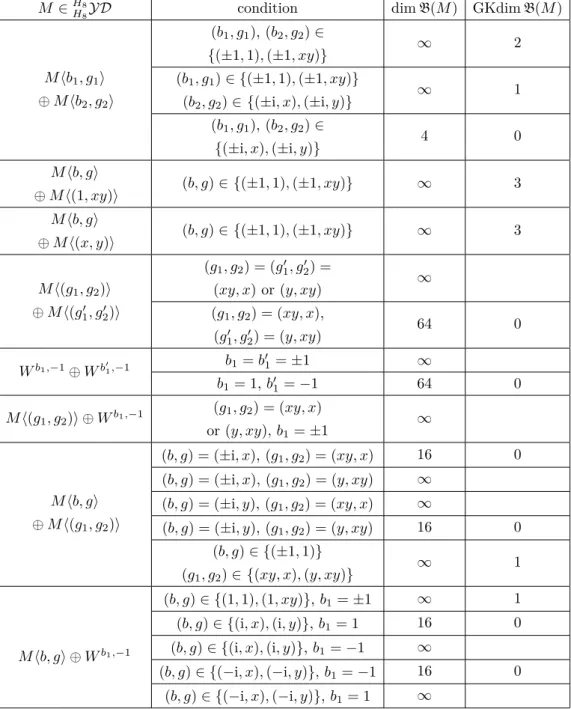
Remark 4.4. According to Propositions 4.1, 4.2, and 4.3, we calculate Nichols algebras over direct sum of two simple objects ofH8

H8YDin Table 3.

Proof of Theorem A. Firstly, we recall the fact that for any submodule M1 ⊂ M2 ∈ H

HYD, B(M1) ⊂ B(M2). Then dimB(M2) = ∞ if dimB(M1) = ∞. The

Nichols algebrasB(M) associated with M listed in Theorem A are finite-dimen-sional according to Lemma 2.3 and [31]. In fact, Ω1(n1, n2, n3, n4) is of Cartan type A1× · · · ×A1

| {z }

n1+n2+n3+n4

; Ωk(n1, n2) for k = 2,3,4,5 is of Cartan type A1× · · · ×A1

| {z }

n1+n2

×A2;

Ωk fork= 6,7 is of Cartan typeA2×A2. So letM ∈HH88YD; then dimB(M)<∞ if and only if M is isomorphic to one of the modules in the list of Theorem A according to Table 2, Table 3, Propositions 4.1 & 4.2.

5. _{Hopf algebras over} H8

In this section, according to the lifting method, we determine the finite-dimen-sional Hopf algebra H with coradical H8 such that its infinitesimal braiding is

isomorphic to a Yetter–Drinfel’d moduleM overH8. We begin by proving thatH

M ∈H8

H8YD condition dimB(M) GKdimB(M)

Mhb1, g1i ⊕Mhb2, g2i

(b1, g1), (b2, g2)∈

{(±1,1),(±1, xy)} ∞ 2

(b1, g1)∈ {(±1,1),(±1, xy)}

(b2, g2)∈ {(±i, x),(±i, y)}

∞ 1

(b1, g1), (b2, g2)∈

{(±i, x),(±i, y)} 4 0 Mhb, gi

⊕Mh(1, xy)i (b, g)∈ {(±1,1),(±1, xy)} ∞ 3 Mhb, gi

⊕Mh(x, y)i (b, g)∈ {(±1,1),(±1, xy)} ∞ 3

Mh(g1, g2)i ⊕Mh(g₁0, g0₂)i

(g1, g2) = (g10, g02) =

(xy, x) or (y, xy) ∞ (g1, g2) = (xy, x),

(g₁0, g₂0) = (y, xy) 64 0

Wb1,−1_⊕Wb01,−1

b1=b0₁=±1 ∞

b1= 1,b01=−1 64 0

Mh(g1, g2)i ⊕Wb1,−1 (g1, g2) = (xy, x)

or (y, xy),b1=±1 ∞

Mhb, gi ⊕Mh(g1, g2)i

(b, g) = (±i, x), (g1, g2) = (xy, x) 16 0

(b, g) = (±i, x), (g1, g2) = (y, xy) ∞

(b, g) = (±i, y), (g1, g2) = (xy, x) ∞

(b, g) = (±i, y), (g1, g2) = (y, xy) 16 0

(b, g)∈ {(±1,1)}

(g1, g2)∈ {(xy, x),(y, xy)} ∞ 1

Mhb, gi ⊕Wb1,−1

(b, g)∈ {(1,1),(1, xy)}, b1=±1 ∞ 1 (b, g)∈ {(i, x),(i, y)},b1= 1 16 0 (b, g)∈ {(i, x),(i, y)},b1=−1 ∞

(b, g)∈ {(−i, x),(−i, y)},b1=−1 16 0

(b, g)∈ {(−i, x),(−i, y)},b1= 1 ∞

Table 3. Nichols algebras over the direct sum of two simple

ob-jects inH8

Theorem 5.1. Let H be a finite-dimensional Hopf algebra over H8 such that its infinitesimal braiding is isomorphic to a Yetter–Drinfel’d module over H8. Then the diagram of H is a Nichols algebra, and consequently H is generated by the elements of degree one with respect to the coradical filtration.

Proof. Since grH ' R#H8, with R = Ln≥0R(n) the diagram of H, we need

to prove that R is a Nichols algebra. Actually we only need to prove that R '

B(M) for some M in the list of Theorem A since R is finite-dimensional. Let

J =L

n≥0R(n)

∗ _{be the graded dual of R; then J is a graded Hopf algebra in}

H8

H8YDwithJ(0) =K1. According to [13, Lemma 5.5],R(1) =P(R) if and only if

J is generated as an algebra by J(1), that is, ifJ is itself a Nichols algebra. Considering B(M) ∈ H8

H8YD for M in the list of Theorem A, since B(M) =

T(M)/I, in order to show that P(J) = J(1) it is enough to prove that the relations that generate the idealI hold inJ. This can be done by a case-by-case computation. We perform here three cases, and leave the rest to the reader.

SupposeM = Ω1(n1, n2, n3, n4). A direct computation shows that the elements rinJ representing the quadratic relations are primitive and they satisfyc(r⊗r) =

r⊗r. As dimJ <∞, it must ber= 0 in J and hence there exists a projective algebra mapB(M)→ J, which implies thatP(J) =J(1).

Suppose M = Ω6; then M is generated by elementsp1 = (v1+v2)xy, p2 =

(v1−v2)x, p0₁ = (v1+v2)y, p0₂ = (v1−v2)xy and the ideal defining the Nichols algebra is generated by the elementsp2

1,p22,p01 2

,p0₂2,p1p2p1p2+p2p1p2p1, p0₁p0₂p₁0p0₂+p0₂p₁0p0₂p0₁, p1p01+p01p1, p1p02+p02p1, p2p01−p01p2, p2p02+p02p2. We can

check directly that all those generators of the defining ideal ofB(M) are primitive elements, or by using [21, Theorem 6]. It is enough to show that c(r⊗r) =

r⊗rfor all generators given above for the defining ideal. Since ρ(p1) = xy⊗p1,

ρ(p2) =x⊗p2,ρ(p₁0) =y⊗p0₁, we haveρ(p2

1) = 1⊗p21, ρ(p1p2p1p2+p2p1p2p1) =

1⊗(p1p2p1p2+p2p1p2p1),ρ(p1p0₁+p₁0p1) =x⊗(p1p0₁+p0₁p1). It is easy to see that

c(r⊗r) =r⊗rholds forr=p₁2,p1p2p1p2+p2p1p2p1, andp1p0₁+p0₁p1. We leave the rest to the reader.

SupposeM = Ω4(n1, n2). ThenM is generated by elementsp1=w 1,−1 1 +iw

1,−1 2 , p2 = w1,₁−1−iw1,₂−1, {Xj}j=1,...,n₁, {Yk}k=1,...,n₂ with _KXj ' Mhi, xi, _KYk ' Mhi, yi and the ideal defining the Nichols algebra is generated by the elements

p2

1, p22, p1p2p1p2+p2p1p2p1, Xj2, {Xj1Xj2 +Xj2Xj1}1≤j1<j2≤n1, Y

2

k, {Yk1Yk2 +

Yk2Yk1}1≤k1<k2≤n2,p1Yk−Ykp1,p2Yk+Ykp2,p1Xj−Xjp1,p2Xj+Xjp2. We can check directly that all those generators of the defining ideal ofB(M) are primitive elements, or by using [21, Theorem 6]. It is enough to show thatc(r⊗r) =r⊗rfor all generators given above for the defining ideal. Sinceρ(p1) = (f00−if11)z⊗p1+

(f10+ if01)z⊗p2,ρ(p2) = (f00+ if11)z⊗p2+ (f10−if01)z⊗p1,ρ(Xj) =x⊗Xj, ρ(p1p2p1p2+p2p1p2p1) = [(f00−if11)z(f00+ if11)z]2⊗p1p2p1p2

+ [(f00+ if11)z(f00−if11)z]2⊗p2p1p2p1

+ [(f10+ if01)z(f10−if01)z]2⊗p2p1p2p1

=xy⊗(p1p2p1p2+p2p1p2p1),

ρ(p1Xj−Xjp1) = (f00+ if11)z⊗(p1Xj−Xjp1) + (f10−if01)z⊗(p2Xj+Xjp2).

Because

(f10−if01)z·(p1Xj−Xjp1)

= f10−if01

2 ·[((1 +y)z·p1)(z·Xj)−((1−y)z·Xj)(xz·p1)] = (−i)(f10−if01)·(p1Xj−Xjp1) = 0,

(f00+ if11)z·(p1Xj−Xjp1) = (−i)(f00+ if11)·(p1Xj−Xjp1) =p1Xj−Xjp1, xy·(p1p2p1p2+p2p1p2p1) =p1p2p1p2+p2p1p2p1,

c(r⊗r) =r⊗rholds forr=p1p2p1p2+p2p1p2p1andp1Xj−Xjp1. We leave the

rest to the reader.

Lemma 5.2 ([13, Lemma 6.1]). Let H be a Hopf algebra, ψ :H →H an auto-morphism of Hopf algebras,V,W Yetter–Drinfel’d modules overH.

(1) Let Vψ be the same space underlying V but with action and coaction h·ψv=ψ(h)·v, ρψ(v) = ψ−1⊗idρ(v), h∈H, v∈V.

Then Vψ is also a Yetter–Drinfel’d module over H. If T : V → W is a morphism in H_HYD, thenTψ : Vψ →Wψ also is. Moreover, the braiding c:Vψ_⊗Wψ_→Wψ_⊗Vψ _{coincides with the braidingc:V ⊗W →W⊗V.}

(2) If R is an algebra (resp., a coalgebra, a Hopf algebra) in H

HYD, then Rψ also is, with the same structural maps.

(3) LetRbe a Hopf algebra inH_HYD. Then the mapΨ :Rψ#H →R#H given byΨ(r#h) =r#ψ(h)is an isomorphism of Hopf algebras.

Corollary 5.3. (1) [Mhbi, xi]τ3 _{'Mh−bi, yi,b=±1.} (2) [Mh(xy, x)i]τ3 _{'Mh(y, xy)i,}

Wb1,−1τ3 '_W−b1,−1 _{with b}

1=±1.

(3) B(Ω2(n1, n2)) #H8'B(Ω3(n2, n1)) #H8,

B(Ω4(n1, n2)) #H8'B(Ω5(n2, n1)) #H8.

LetH be a lifting ofB(Ω1(n1, n2, n3, n4)) #H8. Then there exists an

epimor-phism of Hopf algebras φ:T(Ω1(n1, n2, n3, n4)) #H8 →H [16, Proposition 2.4].

Denote

Xj = (vx)#1, vx∈Mhi, xi, j= 1, . . . , n1, Yk = (vx)#1, vx∈Mh−i, xi, k= 1, . . . , n2,

ps= (vy)#1, vy∈Mhi, yi, s= 1, . . . , n3, qt= (vy)#1, vy∈Mh−i, yi, t= 1, . . . , n4.

(5.1)

Definition 5.4. For n1, n2, n3, n4 ∈N≥0 with n1+n2+n3+n4 ≥1, andI1 = {(λj,s)n1×n3,(θk,t)n2×n4} with entries inK, we denote byA1(n1, n2, n3, n4;I1) the algebra [T(Ω1(n1, n2, n3, n4)) #H8]/I(I1), whereI(I1) is the ideal generated by