arXiv:1803.07404v1 [math-ph] 20 Mar 2018
deformations of Lie–Hamilton systems
based on
sl
(2)
´
Angel Ballesteros, Rutwig Campoamor-Stursberg, Eduardo Fern´andez-Saiz, Francisco J. Herranz and Javier de Lucas
Abstract Based on a recently developed procedure to construct Poisson– Hopf deformations of Lie–Hamilton systems [4], a novel unified approach to nonequivalent deformations of Lie–Hamilton systems on the real plane with a Vessiot–Guldberg Lie algebra isomorphic tosl(2) is proposed. This, in partic-ular, allows us to define a notion of Poisson–Hopf systems in dependence of a parameterized family of Poisson algebra representations. Such an approach is explicitly illustrated by applying it to the three non-diffeomorphic classes of
sl(2) Lie–Hamilton systems. Our results cover deformations of the Ermakov system, Milne–Pinney, Kummer–Schwarz and several Riccati equations as well as of the harmonic oscillator (all of them witht-dependent coefficients). Furthermoret-independent constants of motion are given as well. Our meth-ods can be employed to generate other Lie–Hamilton systems and their de-formations for other Vessiot–Guldberg Lie algebras and their dede-formations.1
´
A. Ballesteros
Departamento de F´ısica, Universidad de Burgos, E-09001 Burgos, Spain, e-mail:[email protected]
R. Campoamor-Stursberg
Instituto de Matem´atica Interdisciplinar I.M.I-U.C.M, Pza. Ciencias 3, E-28040 Madrid, Spain, e-mail:[email protected]
E. Fern´andez-Saiz
Departamento de Geometr´ıa y Topolog´ıa, Universidad Complutense de Madrid, Pza. Ciencias 3, E-28040 Madrid, Spain, e-mail:[email protected]
F.J. Herranz
Departamento de F´ısica, Universidad de Burgos, E-09001 Burgos, Spain, e-mail:[email protected]
J. de Lucas
Department of Mathematical Methods in Physics, University of Warsaw, Pasteura 5, 02-093, Warszawa, Poland, e-mail:[email protected]
1Based on the contribution presented at the “X International Symposium on
Quan-tum Theory and Symmetries” (QTS-10), June 19-25, 2017, Varna, Bulgaria
1 Introduction
Since its original formulation by Lie [23], nonautonomous first-order systems of ordinary differential equations admitting a nonlinear superposition rule, the so-calledLie systems, have been studied extensively (see [11, 13, 16, 20, 27, 28, 31, 32] and references therein). The Lie theorem [14, 23] states that every system of first-order differential equations is a Lie system if and only if it can be described as a curve in a finite-dimensional Lie algebra of vector fields, a referred to asVessiot–Guldberg Lie algebra.
Although being a Lie system is rather an exception than a rule [12, 21, 22], Lie systems have been shown to be of great interest within physical and math-ematical applications (see [16] and references therein). Surprisingly, Lie sys-tems admitting a Vessiot–Guldberg Lie algebra of Hamiltonian vector fields relative to a Poisson structure, the Lie–Hamilton systems, have found even more applications than standard Lie systems with no associated geometric structure [2, 5, 10, 17]. Lie–Hamilton systems admit an additional finite-dimensional Lie algebra of Hamiltonian functions, a Lie–Hamilton algebra, that allows for the algebraic determination of superposition rules and con-stants of motion of the system [10].
Apart from the theory of quasi-Lie systems [12] and superposition rules for nonlinear operators [21, 22], most approaches to Lie systems rely strongly in the theory of Lie algebras and Lie groups [26]. However, the success of quantum groups [18, 24] and the coalgebra formalism within the analysis of superintegrable systems [3, 7, 9], and the fact that quantum algebras appear as deformations of Lie algebras suggested the possibility of extending the no-tion and techniques of Lie–Hamilton systems beyond the range of applicano-tion of the Lie theory. An approach in this direction was recently proposed in [4], where a method to construct quantum deformed Lie–Hamilton systems (LH systems in short) by means of the coalgebra formalism and quantum algebras was given.
The underlying idea is to use the theory of quantum groups to deform Lie systems and their associated structures. More exactly, the deformation transforms a LH system with its Vessiot–Guldberg Lie algebra into a Hamil-tonian system whose dynamics is determined by a set of generators of a Steffan–Sussmann distribution. Meanwhile, the initial Lie–Hamilton algebra (LH algebra in short) is mapped into a Poisson–Hopf algebra. The deformed structures allow for the explicit construction of t-independent constants of the motion through quantum algebra techniques for the deformed system.
func-tions and the corresponding deformed Hamiltonian vector fields, once the corresponding counterpart of the non-deformed system is known.
Moreover this work also provides a new method to construct LH systems with a LH algebra isomorphic to a fixed Lie algebrag. Our approach relies on using the symplectic foliation ing∗induced by the Kirillov–Konstant–Souriou bracket ong. As a particular case, it is explicitly shown how our procedure explains the existence of three types of LH systems on the plane related to a LH algebra isomorphic to sl(2). This is due to the fact that each one of the three different types corresponds to one of the three types of symplectic leaves insl∗(2). Analogously, one can generate the only type of LH systems on the plane admitting a Vessiot–Guldberg Lie algebra isomorphic toso(3). Our systematization permits us to give directly the Poisson–Hopf deformed system from the classification of LH systems [2, 10], further suggesting a notion of Poisson–Hopf Lie systems based on a z-parameterized family of Poisson algebra morphisms. Our methods seem to be extensible to study also LH systems and their deformations on other more general manifolds.
The structure of the contribution goes as follows. Section 2 is devoted to introducing the main aspects of LH systems and Poisson–Hopf algebras. The general approach to construct Poisson–Hopf algebra deformations of LH systems [4] is summarized in Section 3. For our further purposes, the (non-standard) Poisson–Hopf algebra deformation ofsl(2) is recalled in Section 4. The novel unifying approach to deformations of Poisson–Hopf Lie systems with a LH algebra isomorphic to a fixed Lie algebragare treated in Section 5. Such a procedure is explicitly illustrated in Section 6 by applying it to the three non-diffeomorphic classes ofsl(2)-LH systems on the plane, so obtain-ing in a straightforward way their correspondobtain-ing deformation. Next, a new method to construct (non-deformed) LH systems is presented in Section 6. Finally, our results are summarised and the future work to be accomplished is briefly detailed in the last Section.
2 Lie–Hamilton systems and Poisson–Hopf algebras
This section recalls the main notions that will be used in the sequel.
Let {x1, . . . , xn} be global coordinates in Rn and consider a
nonau-tonomous system of first-order ordinary differential equations dxk
dt =fk(t, x1, . . . , xn), 1≤k≤n, (1) where fk : Rn+1 → R are arbitrary functions. Geometrically, this system
Xt:R×Rn∋(t, x1, . . . , xn)7→ n
X
k=1
fk(t, x1, . . . , xn)
∂ ∂xk
∈TRn.
We say that (1) is a Lie system if its general solution, x(t), can be expressed in terms of a finite number m of generic particular solutions
{y1(t), . . . ,ym(t)}and nconstants {C1, . . . , Cn}in the form
x(t) =Ψ(y1(t), . . . ,ym(t), C1, . . . , Cn),
for a certain functionΨ : (Rn)m×Rn→Rn, a so-calledsuperposition ruleof
the system (1).
The Lie–Scheffers Theorem [13, 14, 23, 31] states thatXtis a Lie system if
and only if there existt-dependent functionsb1(t), . . . , br(t) and vector fields
X1, . . . ,Xr onRn spanning anr-dimensional real Lie algebraV such that
Xt(x, y) = r
X
i=1
bi(t)Xi.
Then,V is called aVessiot–Guldberg Lie algebraofXt.
A Lie system is said to be aLie–Hamilton system[17] whenever it admits a Vessiot–Guldberg Lie algebraV of Hamiltonian vector fields with respect to a Poisson structure. In our work, we will focus on LH systems on the plane admitting a Vessiot–Guldberg Lie algebra of Hamiltonian vector fields relative to a symplectic structure. It can be proved that all LH systems can be studied around a generic point in this way [2].
Hence, the LH systems to be studied hereafter admit a symplectic structure ω onR2 that is invariant under Lie derivatives with respect to the elements ofV, namely
LXiω= 0, 1≤i≤r.
Due to the non-degeneracy ofω, each functionhdetermines uniquely a vector fieldXh, theHamiltonian vector fieldofh, such thatιXhω= dh, enabling us
to define a Poisson bracket
{·,·}ω : C∞(R2)×C∞(R2)→C∞(R2)
through the prescription
{f, g}ω7→Xgf. (2)
In particular, this implies that (C∞(R2),{·,·}
ω) is a Lie algebra. Similarly, the
space Ham(ω) of Hamiltonian vector fields onR2relative toωis a Lie algebra with respect to the commutator of vector fields. These two Lie algebras are known to be related through the exact sequence (see [29] for details):
0֒→R֒→(C∞(R2),{·,·}ω) ϕ
−→(Ham(ω),[·,·])−→π 0,
whereϕmaps every functionh∈C∞(R2) into−X
Going back to the theory of LH systems, recall that every LH system admits a Vessiot–Guldberg Lie algebraV of Hamiltonian vector fields relative to anω. In view of (2), there always exists a finite-dimensional Lie subalgebra
Hωof (C∞(R2),{·,·}ω) containing the Hamiltonian functions ofV: a so-called
Lie–Hamilton algebraof the LH systemXt.
Letg be a Lie algebra isomorphic to Hω. This induces the universal
en-veloping algebra U(g) and the symmetric algebra S(g) (see [30] for details). The second one is the associative commutative algebra of polynomials in the elements ofg, whereasU(g) is defined to be the tensor algebra ofgmodulo the two-sided ideal generated by the elements{v⊗w−w⊗v−[v, w] :v, w∈g}. Relevantly,S(g) andU(g) are isomorphic as linear spaces [30]. They also share a special property: they are Hopf algebras. The Lie bracket ofgcan be extended toS(g) turning this space into a Poisson algebra. Since the elements of gcan be considered as linear functions on g∗, then the elements of S(g) can be considered as elements ofC∞(g∗), which allows us to ensure that the spaceC∞(g∗) can be endowed with aPoisson–Hopf algebrastructure.
Let us finally recall in this introduction the main properties of Hopf alge-bras. We recall that an associative algebraAwith aproductmand aunitηis said to be aHopf algebraoverR[1, 18, 24] if there exist two homomorphisms calledcoproduct (∆:A−→A⊗A) andcounit(ǫ:A−→R) satisfying
(Id⊗∆)∆= (∆⊗Id)∆, (Id⊗ǫ)∆= (ǫ⊗Id)∆= Id,
along with an antihomomorphism, the antipode γ :A −→A, such that the following diagram is commutative:
A⊗AId⊗γ/ /A⊗A
m
✼ ✼ ✼ ✼ ✼ ✼
A
∆
✼ ✼ ✼ ✼ ✼ ✼ ✼
ǫ /
/
∆
C
C
✟ ✟ ✟ ✟ ✟ ✟
R η / /A
A⊗Aγ⊗Id/ /A⊗A
m
C
C
✟ ✟ ✟ ✟ ✟ ✟ ✟
3 Poisson–Hopf deformations of Lie–Hamilton systems
The coalgebra method employed in [5] to obtain superposition rules and constants of motion for LH systems on a manifoldM relies almost uniquely in the Poisson–Hopf algebra structure related toC∞(g∗) and a Poisson map
D:C∞(g∗)→C∞(M),
where we recall that gis a Lie algebra isomorphic to a LH algebra,Hω, of
Relevantly, quantum deformations allow us to repeat this scheme by sub-stituting the Poisson algebraC∞(g∗) with a quantum deformationC∞(g∗
z),
wherez∈R, and obtaining an adequate Poisson map
Dz:C∞(g∗z)→C
∞(M).
The above procedure enables us to deform the LH system into a z -parametric family of Hamiltonian systems whose dynamic is determined by a Steffan–Sussmann distribution and a family of Poisson algebras. Ifz tends to zero, then the properties of the (classical) LH system are recovered by a limiting process, hence enabling to construct new deformations exhibiting physically relevant properties.
In essence, the method for a LH system on ann-dimensional manifoldM consists essentially of the following four steps (see [4] for details):
1. Consider a LH systemXt :=Pr
i=1bi(t)Xi onM with respect to a
sym-plectic formω and possessing a LH algebraHω spanned by the functions
{h1, . . . , hr} ⊂C∞(M) and structure constantsCijk, i.e.
{hi, hj}ω= r
X
k=1
Cijkhk, 1≤i, j≤r.
2. Consider a Poisson–Hopf algebra deformationC∞(H∗
z,ω) with (quantum)
deformation parameterz∈R(respectivelyq:= ez) as the space of smooth
functions F(hz,1, . . . , hz,r) for a family of functions hz,1, . . . , hz,r on M
such that
{hz,i, hz,j}ω=Fz,ij(hz,1, . . . , hz,r), (3)
where the Fz,ij are smooth functions depending also on z satisfying the
boundary conditions
lim
z→0hz,i=hi, zlim→0gradhz,i= gradhi, lim
z→0Fz,ij(hz,1, . . . , hz,r) =
r
X
k=1
Cijkhk. (4)
3. Define the deformed vector fieldsXz,i onM according to the rule
ιXz,iω= dhz,i, (5)
so that
lim
z→0Xz,i=Xi. (6) 4. Define the Poisson–Hopf deformation of the LH systemXt as
Xz,t:= r
X
i=1
We stress that the deformed vector fields {Xz,1, . . . ,Xz,r} do not
gener-ally close on a finite-dimensional Lie algebra. Instead, they span a Stefan– Sussman distribution (see [15, 27, 29]). Their corresponding commutation relations can be written in terms of the functionsFz,ij as [4]
[Xz,i,Xz,j] =−
r
X
k=1 ∂Fz,ij
∂hz,k
Xz,k. (7)
Next, to determine the t-independent constants of the motion and the superposition rules of a LH system with a LH algebra Hω, the coalgebra
formalism developed in [5] is applied. Let us illustrate this point. Consider the symmetric algebraS(g) ofg≃ Hω, that can be endowed with a Poisson
algebra structure by means of the Lie algebra structure ofg. The Hopf algebra structure with a (non-deformed trivial) coproduct map∆ is given by
∆:S(g)→S(g)⊗S(g), ∆(v) :=v⊗1 + 1⊗v, ∀v∈g.
This is easily seen to be a Poisson algebra homomorphism with respect to the Poisson structure on S(g) and the natural Poisson structure in S(g)⊗
S(g) induced by S(g). Due to density of the functions S(g) in C∞(g∗), the coproduct∆ can be extended in a unique way to
∆:C∞(g∗)→C∞(g∗)⊗C∞(g∗).
The extension by continuity of the Poisson–Hopf structure inS(g) toC∞(g∗) endows the latter with a Poisson–Hopf algebra structure [5].
Let nowC =C(v1, . . . , vr) be a Casimir function of the Poisson algebra
C∞(g∗), wherev1, . . . , v
r is a basis forg. We can define a Lie algebra
mor-phismφ:g→C∞(M) such thath
i:=φ(vi). The Poisson algebra morphisms
D:C∞(g∗)→C∞(M), D(2):C∞(g∗)⊗C∞(g∗)→C∞(M)⊗C∞(M),
defined by
D(vi) :=hi(x1), D(2)(∆(vi)) :=hi(x1) +hi(x2), 1≤i≤r,
where xs = {xs,1, . . . , xs,n} (s = 1,2) are global coordinates in M, lead to
t-independent constants of the motionF(1):=F andF(2) ofX
t having the
form
F :=D(C), F(2):=D(2)(∆(C)). (8) The very same argument holds to any deformed Poisson–Hopf alge-bra C∞(g∗
z) with deformed coproduct ∆z and Casimir invariant Cz =
Cz(vz,1, . . . , vz,r), where {vz,1, . . . , vz,r} satisfy the same formal
commuta-tion relacommuta-tions of thehz,i in (3), and such that
lim
Therefore, the deformed CasimirCzwill provide thet-independent constants
of motion for the deformed LH systemXz,t through the coproduct∆z.
4 The non-standard Poisson–Hopf algebra deformation
of
sl
(2)
Amongst the LH systems in the plane (see [2, 5, 10] for details and applica-tions), those with a Vessiot–Guldberg Lie algebra isomorphic tosl(2) are of both mathematical and physical interest; they cover complex Riccati, Milne– Pinney and Kummer–Schwarz equations as well as the harmonic oscillator, all of them witht-dependent coefficients. Furthermore,sl(2)-LH systems are re-lated to three non-diffeomorphic Vessiot–Guldberg Lie algebras on the plane [2, 10]. This gives rise to different nonequivalent Poisson–Hopf deformations. Let us consider sl(2) with the standard basis {J3, J+, J−} satisfying the commutation relations
[J3, J±] =±2J±, [J+, J−] =J3.
In this basis, the Casimir operator reads
C= 1 2J
2
3 + (J+J−+J−J+). (9)
Considering the non-standard (triangular or Jordanian) quantum deforma-tionUz(sl(2)) ofsl(2) [25] (see also [6, 8] and references therein), we are led
to the following deformed coproduct
∆z(J+) =J+⊗1 + 1⊗J+,
∆z(Jl) =Jl⊗e2zJ++ e−2zJ+⊗Jl, l∈ {−,3}
and the commutation rules
[J3, J+]z= 2 shc(2zJ+)J+, [J+, J−]z=J3, [J3, J−]z=−J−ch(2zJ+)−ch(2zJ+)J−.
Here shc denotes the cardinal hyperbolic sinus function defined by
shc(ξ) := ( sh(
ξ)
ξ , forξ6= 0,
1, forξ= 0.
It is known that every quantum algebraUz(g) related to a semi-simple Lie
algebragadmits an isomorphism of algebrasUz(g)→U(g) (see [18, Theorem
6.1.8]). This allows us to obtain a Casimir operator ofUz(sl(2)) out of one,
Cz=
1 2J
2
3+ shc(2zJ+)J+J−+J−J+shc(2zJ+) + 1 2ch
2(2zJ+),
which, as expected, coincides with the expression formerly given in [8]. There exists a newz-parametrized family of deformed Poisson–Hopf struc-tures inC∞(sl∗
z(2)) denoted by (C∞(sl
∗
z(2)),{·,·}z) and given by the relations
{v1, v2}z=−shc(2zv1)v1, {v1, v3}z=−2v2, {v2, v3}z=−ch(2zv1)v3,
(10) along with the coproduct
∆z(v1) =v1⊗1+1⊗v1, ∆z(vk) =vk⊗e2zv1+e−2zv1⊗vk, k= 2,3. (11)
The Poisson algebraC∞(sl
z(2)) admits a Casimir function
Cz= shc(2zv1)v1v3−v22, (12)
where
v1=J+, v2= 1
2J3, v3=−J−. (13)
In the limitz= 0, the Poisson–Hopf structure inC∞(sl∗
z(2)) recovers the
standard Poisson–Hopf algebra structure in C∞(sl∗
(2)) with non-deformed coproduct and Poisson bracket
∆(vi) =vi⊗1 + 1⊗vi, i= 1,2,3,
{v1, v2}=−v1, {v1, v3}=−2v2, {v2, v3}=−v3, (14)
as well as the Casimir function
C=v1v3−v22. (15)
We shall make use of the above Poisson–Hopf algebraC∞(sl∗
z(2)) in the
next section in order to construct the corresponding deformed LH systems from a unified approach.
5 Poisson–Hopf deformations of
sl
(2) Lie–Hamilton
systems
Let us endow a manifoldM with a symplectic structureω and consider a Hamiltonian Lie group actionΦ:SL(2,R)×M →M. A basis of fundamental vector fields ofΦ, let us say{X1,X2,X3}, enable us to define a Lie system
Xt=
3 X
i=1
bi(t)Xi,
for arbitraryt-dependent functionsb1(t), b2(t), b3(t), and{X1,X2,X3} span-ning a Lie algebra isomorphic tosl(2). As is well known, there are only three non-diffeomorphic classes of Lie algebras of Hamiltonian vector fields iso-morphic to sl(2) on the plane [2, 19]. Since X1,X2,X3 admit Hamiltonian functions h1, h2, h3, the t-dependent vector field X admits a t-dependent Hamiltonian function
h= 3 X
i=1 bi(t)hi.
Due to the cohomological properties ofsl(2) (see e.g. [29]), the Hamiltonian functionsh1, h2, h3can always be chosen so that the spacehh1, h2, h3ispans a Lie algebra isomorphic tosl(2) with respect to{·,·}ω.
Let{v1, v2, v3}be the basis forsl(2) given in (13) and letM be a manifold where the functionsh1, h2, h3are smooth. Further, the Poisson–Hopf algebra structure of C∞(sl∗
(2)) is given by (14). In these conditions, there exists a Poisson algebra morphismD:C∞(sl∗
(2))→C∞(M) satisfying
D(f(v1, v2, v3)) =f(h1, h2, h3), ∀f ∈C∞(sl∗(2)).
Recall that the deformationC∞(sl∗
z(2)) ofC∞(sl
∗
(2)) is a Poisson–Hopf al-gebra with the new Poisson structure induced by the relations (10). Let us define the submanifold O =: {θ ∈ sl∗(2) : v1(θ) 6= 0} of sl∗(2). Then, the Poisson structure onsl∗(2) can be restricted to the spaceC∞(O). In turn, this enables us to expand the Poisson–Hopf algebra structure inC∞(sl∗
(2)) toC∞(O). Within the latter space, the elements
vz,1:=v1, vz,2:= shc(2zv1)v2,
vz,3:= shc(2zv1)v 2 2 v1 +
c
4 shc(2zv1)v1, (16) are easily verified to satisfy the same commutation relations with respect to
{·,·}as the elementsv1, v2, v3in C∞(sl∗
z(2)) with respect to{·,·}z (10), i.e.
{vz,1, vz,2}=−shc(2zvz,1)vz,1, {vz,1, vz,3}=−2vz,2,
{vz,2, vz,3}=−ch(2zvz,1)vz,3. (17)
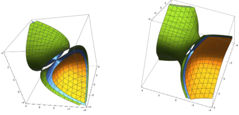
Fig. 1 Representatives of the submanifolds insl∗(2) given by the surfaces with con-stant value of the Casimir for the Poisson structure insl∗(2) (left) and its deformation (right). Such submanifolds are symplectic submanifolds where the Poisson bivectors
ΛandΛzadmit a canonical form.
{v0,1, v0,2}=−v0,1, {v0,1, v0,3}= 2{v0,1, v0,2}v0,2
v0,1 =−2v0,2,
{v0,2, v0,3}=− v2
0,2 v2
0,1
{v0,2, v0,1} − c 4v2
0,1
{v0,2, v0,1}=− v2
0,2 v0,1
− c
4v0,1
=−v0,3.
The functionsvz,1, vz,2, vz,3are not functionally independent, as they satisfy the constraint
shc(2zv1,z)v1,zv3,z−v22,z =c/4. (18)
The existence of the functionsvz,1, vz,2, vz,3and the relation (18) with the Casimir of the deformed Poisson–Hopf algebra is by no means casual. Let us explain why vz,1, vz,2, vz,3 exist and how to obtain them easily.
Around a generic pointp∈sl∗(2), there always exists an openUp
contain-ing pwhere both Poisson structures give a symplectic foliation by surfaces. Examples of symplectic leaves for{·,·}and{·,·}z are displayed in Fig. 1.
The splitting theorem on Poisson manifolds [29] ensure that if Up is
small enough, then there exist two different coordinate systems {x, y, C}
and{xz, yz, Cz} where the Poisson bivectors related to{·,·}and{·,·}zread
Λ = ∂x∧∂y and Λz = ∂xz ∧∂yz. Hence, Cz and C are Casimir functions
forΛzandΛ, respectively. Moreover,xz=xz(x, y, C), yz=yz(x, y, C), Cz=
Cz(x, y, C). It follows from this that
Φ:f(xz, yz, Cz)∈Cz∞(Up)7→f(x, y, C)∈C∞(Up)
is a Poisson algebra morphism.
R3→R. Hence, the ˆvz,i=ξi(x, y, C) close the same commutation relations
relative to{·,·}as thevido with respect to{·,·}z. AsCis a Casimir invariant,
the functionsvz,i:=ξi(x, y, c), with a constant value ofc, still close the same
commutation relations among themselves as the vi. Moreover, the functions
vz,i become functionally dependent. Indeed,
Cz=Cz(v1, v2, v3) =Cz(ξ1(xz, yz, Cz), ξ2(xz, yz, Cz), ξ3(xz, yz, Cz)).
Hence, c = Cz(ξ1(xz, yz, c), ξ2(xz, yz, c), ξ3(xz, yz, c)) and we conclude that
c=Cz(vz,1, vz,2, vz,3).
The previous argument allows us to recover the functions (16) in an al-gorithmic way. Actually, the functions xz, yz, Cz and x, y, C can be easily
chosen to be
xz:=v1, yz:=−
v2
shc(2zv1)v1, Cz:= shc(2zv1)v1v3−v 2 2,
as well as
x=v1, y =−v2/v1, C=v1v3−v22. Therefore,
ξ1(xz, yz, Cz) =xz, ξ2(xz, yz, Cz) =−yzshc(2zxz)xz,
ξ3(xz, yz, Cz) =
Cz+x2zyz2shc
2(2zx
z)
shc(2zxz)xz
.
Assuming thatCz=c/4, replacingxz, yzbyx=v1, y=−v2/v1, respectively,
and taking into account thatvz,i:=ξi(x, y, c), one retrieves (16).
It is worth mentioning that due to the simple form of the Poisson bivectors in splitting form for three-dimensional Lie algebras, this method can be easily applied to such a type of Lie algebras.
Next, the above relations enable us to construct a Poisson algebra mor-phism
Dz:f(v1, v2, v3)∈C∞(sl∗z(2))7→D(f(v1,z, v2,z, v3,z))∈C∞(M)
for every value of z allowing us to pass the structure of the Poisson–Hopf algebraC∞(sl∗
z(2)) toC∞(M). As a consequence,Dz(Cz) satisfies the
rela-tions
{Dz(Cz), hz,i}ω= 0, i= 1,2,3.
Using the symplectic structure onM and the functionshz,iwritten in terms
of{h1, h2, h3}, one can easily obtain the deformed vector fieldsXz,iin terms
of the vector fieldsXi. Finally, asXz,t=Pi3=1bi(t)Xz,iholds, it is
straight-forward to verify that the brackets
imply that the functionD(Cz) is at-independent constant of the motion for
each of the deformed LH systemXz,t.
Consequently, deformations of LH-systems based on sl(2) can be treated simultaneously, starting from their classical LH counterpart. The final result is summarized in the following statement.
Theorem 1.If φ : sl(2) → C∞(M) is a morphism of Lie algebras with respect to the Lie bracket in sl(2) and a Poisson bracket in C∞(M), then for each z ∈Rthere exists a Poisson algebra morphism Dz :C∞(sl∗z(2))→
C∞(M)such that for a basis{v1, v2, v3}satisfying the commutation relations (14) is given by
Dz(f(v1, v2, v3))
=f
φ(v1),shc(2zφ(v1))φ(v2), shc(2zφ(v1))φ 2(v2) φ(v1) +
c
4 shc(2zφ(v1))φ(v1)
.
Provided thathi:=φ(vi), the deformed Hamiltonian functionshz,i:=Dz(vi)
adopt the form
hz,1=h1, hz,2= shc(2zh1)h2,
hz,3= shc(2zh1) h2
2 h1+
c 4 shc(2zh1)h1, which satisfy the commutation relations (17).
The Hamiltonian vector fields Xz,i associated with hz,i through (5) turn
out to be
Xz,1=X1, Xz,2= h2
h1 ch(2zh1)− shc(2zh1)
X1+ shc(2zh1)X2,
Xz,3= h2
2 h2 1
ch(2zh1)−2 shc(2zh1)
− cch(2zh1)
4h2 1shc
2(2zh1)
X1
+2h2
h1 shc(2zh1)X2,
and satisfy the following commutation relations coming from (7)
[Xz,1,Xz,2] = ch(2zhz,1)Xz,1, [Xz,1,Xz,3] = 2Xz,2,
[Xz,2,Xz,3] = ch(2zhz,1)Xz,3+ 4z2shc2(2zhz,1)hz,1hz,3Xz,1.
As a consequence, the deformed Poisson–Hopf system can be generically described in terms of the Vessiot–Guldberg Lie algebra corresponding to the non-deformed LH system as follows:
Xz,t=
3 X
i=1
bi(t)Xz,i=
b1(t) +b2(t)h2
h1 ch(2zh1)−shc(2zh1)
+b3(t)
h2 2 h2 1
ch(2zh1)−2 shc(2zh1)
− cch(2zh1)
4h2 1shc
2 (2zh1)
X1
+ shc(2zh1)
b2(t) + 2b3(t)h2 h1
X2.
This unified approach to nonequivalent deformations of LH systems pos-sessing a common underlying Lie algebra suggests the following definition.
Definition 1.Let (C∞(M),{·,·}) be a Poisson algebra. A Poisson–Hopf Lie system is pair consisting of a Poisson–Hopf algebra C∞(g∗
z) and a z
-parametrized family of Poisson algebra representations Dz : C∞(g∗z) →
C∞(M) withz∈ R.
Next, constants of the motion for Xz,t can be deduced by applying the
coalgebra approach introduced in [5] in the way briefly described in Section 3. In the deformed case, we consider the Poisson algebra morphisms
Dz:C∞(slz∗(2))→C∞(M),
D(2)z :C∞(
sl∗z(2))⊗C∞(
sl∗z(2))→C∞(M)⊗C∞(M), which by taking into account the coproduct (11) are defined by
Dz(vi) :=hz,i(x1)≡h(1)z,i, i= 1,2,3, D(2)z (∆z(v1)) =hz,1(x1) +hz,1(x2)≡h(2)z,1,
D(2)z (∆z(vk)) =hz,k(x1)e2zhz,1(x2)+ e−2zhz,1(x1)hz,k(x2)≡h(2)z,k, k= 2,3, where xs (s = 1,2) are global coordinates in M. We remark that, by
con-struction, the functions h(2)z,i satisfy the same Poisson brackets (17). Then t-independent constants of motion are given by (see (8))
Fz≡Fz(1) :=Dz(Cz), Fz(2):=D(2)z (∆z(Cz)),
whereCz is the deformed Casimir (12). Explicilty, they read
Fz= shc
2zh(1)z,1h(1)z,1hz,(1)3−h(1)z,22= c 4, Fz(2)= shc
2zh(2)z,1
h(2)z,1h
(2)
z,3−
h(2)z,2 2
.
6 The three classes of
sl
(2) Lie–Hamilton systems on
the plane and their deformation
Table 1 The three classes of LH systems on the plane with underlying Vessiot– Guldberg Lie algebra isomorphic tosl(2). For each class, it is displayed, in this order, a basis of vector fieldsXi, Hamiltonian functionshi, symplectic formω, the constants of motionF andF(2)as well as the corresponding specific LH systems.
•Class P2withc= 4>0
X1= ∂
∂x X2=x ∂ ∂x +y
∂
∂y X3= (x
2−y2) ∂ ∂x + 2xy
∂ ∂y
h1=−1
y h2=− x
y h3=− x2+y2
y ω=
dx∧dy
y2
F= 1 F(2)= (x1−x2)2+ (y1+y2)2 y1y2
– Complex Riccati equation
– Ermakov system, Milne–Pinney and Kummer–Schwarz equations withc >0
•Class I4withc=−1<0
X1= ∂ ∂x+
∂
∂y X2=x ∂ ∂x +y
∂
∂y X3=x 2 ∂
∂x+y 2 ∂
∂y
h1=
1
x−y h2=
x+y
2(x−y) h3=
xy
x−y ω=
dx∧dy (x−y)2
F=−1 4 F
(2)=−(x2−y1)(x1−y2)
(x1−y1)(x2−y2)
– Split-complex Riccati equation
– Ermakov system, Milne–Pinney and Kummer–Schwarz equations withc <0 – Coupled Riccati equations
•Class I5withc= 0
X1= ∂
∂x X2=x ∂ ∂x +
y
2
∂
∂y X3=x 2 ∂
∂x+xy ∂ ∂y
h1=− 1
2y2 h2=− x
2y2 h3=− x2
2y2 ω=
dx∧dy
y3
F= 0 F(2)= (x1−x2)2
4y2 1y22
– Dual-Study Riccati equation
– Ermakov system, Milne–Pinney and Kummer–Schwarz equations withc= 0 – Harmonic oscillator
– Planar diffusion Riccati system
local classification performed in [2], which was based in the results formerly given in [19]. Thus the manifold M = R2 and the coordinates x = (x, y). According to [2, 10], these three classes are named P2, I4 and I5 and they correspond to a positive, negative and zero value of the Casimir constantc, respectively. Recall that these are non-diffeomorphic, so that there does not exist any localt-independent change of variables mapping one into another.
Table 2 Poisson–Hopf deformations of the three classes ofsl(2)-LH systems written in Table 1. The symplectic formωis the same given in Table 1 andF≡Fz.
•Class P2withc= 4>0
Xz,1= ∂
∂x Xz,2=xch(2z/y) ∂
∂x +yshc(2z/y) ∂ ∂y
Xz,3=
x2− y2
shc2(2z/y)
ch(2z/y) ∂
∂x+ 2xyshc(2z/y) ∂ ∂y
hz,1=−1
y hz,2=− x
yshc(2z/y) hz,3=−
x2shc2(2z/y) +y2 yshc(2z/y)
F(2)
z =
(x1−x2)2 y1y2
shc(2z/y1) shc(2z/y2) e2z/y1e−2z/y2
+(y1+y2)
2
y1y2
shc2(2z/y
1+ 2z/y2)
shc(2z/y1) shc(2z/y2)
e2z/y1e−2z/y2
•Class I4withc=−1<0
Xz,1= ∂ ∂x+
∂ ∂y
Xz,2= x+y
2 ch
2z
x−y
∂ ∂x +
∂ ∂y
+x−y 2 shc
2z
x−y
∂ ∂x−
∂ ∂y
Xz,3= 1
4ch
2z
x−y (x+y)
2+ (x−y)2shc−2
2z
x−y
∂ ∂x+ ∂ ∂y +1 2(x−y)
2shc 2z x−y
∂ ∂x −
∂ ∂y
hz,1=
1
x−y hz,2=
(x+y) shc 2z
x−y
2(x−y) hz,3=
(x+y)2shc22z
x−y
−(x−y)2
4(x−y) shc
2z
x−y
Fz(2)=
(x1−x2+y1−y2)2 4(x1−y1)(x2−y2)
shc
2z
x1−y1
shc
2z
x2−y2
e−
2z x1−y1e
2z x2−y2
−
(x1+x2−y1−y2) shc
2z
x1−y1 +
2z
x2−y2
4(x1−y1)(x2−y2)
ex22−zy2(x1−y1) shc 2z
x1−y1
+
e−x2z
1−y1(x2−y2) shc 2z
x2−y2
•Class I5withc= 0
Xz,1= ∂
∂x Xz,2=xch z/y 2 ∂
∂x+ y
2shcz/y
2 ∂
∂y
Xz,3=x2ch z/y2 ∂
∂x+xyshc z/y 2 ∂
∂y
hz,1=− 1
2y2 hz,2=− x
2y2shc z/y 2
hz,3=−x
2
2y2shcz/y 2
F(2)
z =
(x1−x2)2
4y2 1y22
shc z/y2 1
shc z/y2 2
ez/y2 1e−z/y
2 2
[X1,X2] =X1, [X1,X3] = 2X2, [X2,X3] =X3,
{h1, h2}ω=−h1, {h1, h3}ω=−2h2, {h2, h3}ω=−h3.
By applying Theorem 1 with the results of Table 1 we obtain the corre-sponding deformations which are displayed in Table 2. It is straightforward to verify that the classical limitz→0 in Table 2 recovers the corresponding starting LH systems and related structures of Table 1, in agreement with the relations (4) and (6).
7 A method to construct Lie–Hamilton systems
Section 5 showed that deformations of a LH system with a fixed LH algebra
Hω≃gcan be obtained through a Poisson algebraC∞(g∗), a given
deforma-tion and a certain Poisson morphism D : C∞(g∗)→ C∞(M). This section presents a simple method to obtainDfrom an arbitraryg∗onto a symplectic manifoldR2n.
Theorem 2.Letgbe a Lie algebra whose Kostant–Kirillov–Souriau Poisson bracket admits a symplectic foliation in g∗ with a 2n-dimensional S ⊂ g∗. Then, there exists a LH algebra on the plane given by
Φ:g→C∞ R2n
relative to the canonical Poisson bracket on the plane.
Proof. The Lie algebraggives rise to a Poisson structure ong∗through the Kostant–Kirillov–Souriau bracket {·,·}. This induces a symplectic foliation on g∗, whose leaves are symplectic manifolds relative to the restriction of the Poisson bracket. Such leaves are characterized by means of the Casimir functions of the Poisson bracket. By assumption, one of these leaves is 2n -dimensional. In such a case, the Darboux Theorem warrants that the Poisson bracket on each leave is locally symplectomorphic to the Poisson bracket of the canonical symplectic form on R2n ≃ T∗
Rn. In particular, there exists some Darboux coordinates mapping the Poisson bracket on such a leaf into the canonical symplectic bracket onT∗
Rn. The corresponding change of vari-ables into the canonical form in Darboux coordinates can be understood as a local diffeomorphismh:Sk→R2n mapping the Poisson bracketΛkon the
leafSk into the canonical Poisson bracket onT∗Rn. Hence,hgives rise to a
canonical Poisson algebra morphismφh:C∞(Sk)→C∞(T∗Rn).
As usual, a basis{v1, . . . , vr}ofgcan be considered as a coordinate system
ong∗. In view of the definition of the Kostant–Kirillov–Souriau bracket, they span anr-dimensional Lie algebra. In fact, if [vi, vj] =Prk=1ckijvk for certain
constants ck
ij, then{vi, vj}=Pkr=1ckijvk. SinceSk is a symplectic
morphism. In consequence,
{ι∗vi, ι∗vj}= r
X
k=1 ckijι
∗ vk.
Hence, the functionsι∗v
ispan a finite-dimensional Lie algebra of functions on
S. SinceSis 2n-dimensional, there exists a local diffeomorphismφ:S →R2n and
Φ:v∈g7→φ◦ι∗v ∈C∞ R2n is a Lie algebra morphism.
Let us apply the above to explain the existence of three types of LH systems on the plane. We already know that the Lie algebra sl(2) gives rise to a Poisson algebra inC∞(g∗). In the standard basisv1, v2, v3with commutation relations (14), the Casimir is (15). It turns out that the symplectic leaves of this Casimir are of three types:
• A one-sheet hyperboloid whenv1v3−v22=k <0.
• A conical surface whenv1v3−v22= 0.
• A two-sheet hyperboloid whenv1v3−v22=k >0. In each of the three cases we have the Poisson bivector
Λ=−v1 ∂ ∂v1 ∧
∂ ∂v2 −2v2
∂ ∂v1 ∧
∂ ∂v3−v3
∂ ∂v2 ∧
∂ ∂v3.
Then, we have a changes of variables passing from the above form into Dar-boux coordinates
¯
v1=v1, v2¯ =−v2/v1, C=v1v3−v2 2. Then,
v1=v1, v2=−¯v1¯v2, v3= (C+ ¯v12v¯22)/¯v1.
On a symplectic leaf, the value of C is constant, say C = c/4, and the restrictions of the previous functions to the leaf read
ι∗v1=v1, ι∗v2=−¯v1v2,¯ ι∗v3=c/(4¯v1) + ¯v1v¯2 2. This can be viewed as a mappingΦ:sl(2)→C∞(
R2) such that
φ(v1) =x, φ(v2) =−xy, φ(v3) =c/(4x) +xy2,
variables onR2mapping one set of variables into another for different values ofc. Hence, Theorem 2 ultimately explains the real origin of all thesl(2)-LH systems on the plane.
It is known that su(2) admits a unique Casimir, up to a proportional constant, and the symplectic leaves induced insu∗(2) are spheres. The appli-cation of the previous method originates a unique Lie algebra representation, which gives rise to the unique LH system on the plane related toso(3). All the remaining LH systems on the plane can be generated in a similar fashion. The deformations of such Lie algebras will generate all the possible deformations of LH systems on the plane.
8 Concluding remarks
It has been shown that Poisson–Hopf deformations of LH systems based on the simple Lie algebrasl(2) can be formulated simultaneously by means of a geometrical argument, hence providing a generic description for the deformed Hamiltonian functions and vectors fields, starting from the corresponding classical counterpart. This allows for a direct determination of the deformed Hamiltonian functions and vector fields, as well as their corresponding Pois-son brackets and commutators, by mere insertion of the data corresponding to the non-deformed LH system. This procedure has been explicitly illus-trated by obtaining the deformed results of Table 2 from the classical ones of Table 1 through the application of Theorem 1.
Moreover we have explained a method to obtain (non-deformed) LH sys-tems related to a LH algebra Hω by using the symplectic foliation in g∗,
where gis isomorphic to Hω, which has been stated in Theorem 2. This
re-sult could further be applied in order to obtain deformations of LH systems beyondsl(2). It is also left to accomplish the deformation of LH systems in other spaces of higher dimension.
It seems that the techniques provided here are potentially sufficient to provide a solution to the above mentioned problems. These will be the subject of further work currently in progress.
References
1. E. Abe,Hopf Algebras, Cambridge Tracts in Mathematics74(Cambridge: Cam-bridge Univ. Press, 1980)
2. A. Ballesteros, A. Blasco, F.J. Herranz, J de Lucas, C. Sard´on, J. Differential Equations258(2015) 2873–2907
3. A. Ballesteros, A. Blasco, F.J. Herranz, F. Musso, O. Ragnisco, J. Phys.: Conf. Ser.175(2009) 012004
4. A. Ballesteros, R. Campoamor-Stursberg, E. Fern´andez-Saiz, F.J. Herranz, J. de Lucas, J. Phys. A: Math. Theor.51(2018) 065202
5. A. Ballesteros, J.F. Cari˜nena, F.J. Herranz, J. de Lucas, C. Sard´on, J. Phys. A: Math. Theor.46(2013) 285203
6. A. Ballesteros, F.J. Herranz, J. Phys. A: Math. Gen.29(1996) L311–L316 7. A. Ballesteros, F.J. Herranz, O. Ragnisco, J. Phys. A: Math. Gen. 38 (2005)
7129–7144
8. A. Ballesteros, F.J. Herranz, M. del Olmo, M. Santander, J. Phys. A: Math. Gen.
28(1995) 941–955
9. A. Ballesteros, O. Ragnisco, J. Phys. A: Math. Gen.31(1998) 3791–3813 10. A. Blasco A, F.J. Herranz, J. de Lucas, C. Sard´on, J. Phys. A: Math. Theor.48
(2015) 345202
11. R. Campoamor-Stursberg, J. Math. Phys.57(2016) 063508
12. J.F. Cari˜nena, J. Grabowski, J. de Lucas, J. Phys. A: Math. Theor.43(2010) 305201
13. J.F. Cari˜nena, J. Grabowski, G. Marmo, Lie–Scheffers Systems: a Geometric Approach(Bibliopolis, Naples, 2000)
14. J.F. Cari˜nena, J. Grabowski, G. Marmo, Rep. Math. Phys.60(2000) 237–258 15. J.F. Cari˜nena, A. Ibort, G. Marmo, G. Morandi,Geometry from Dynamics,
Clas-sical and Quantum(Springer, New York, 2015)
16. J.F. Cari˜nena, J. Lucas,Dissertations Math. (Rozprawy Mat.)479(2011) 1–162 17. J.F. Cari˜nena, J. de Lucas, C. Sard´on, Int. J. Geom. Methods Mod. Phys.10
(2013) 1350047
18. V. Chari, A. Pressley, A Guide to Quantum Groups(Cambridge Univ. Press, Cambridge, 1994)
19. A. Gonz´alez-L´opez, N. Kamran, P.J. Olver, Proc. London Math. Soc.64(1992) 339–368
20. N.H. Ibragimov, A.A. Gainetdinova, Int. J. Non-linear Mech.90(2017) 50–71 21. A. Inselberg,On classification and superposition principles for nonlinear
opera-tors, Thesis (Ph.D.), University of Illinois at Urbana-Champaign, ProQuest LLC, Ann Arbor, MI, 1965
22. A. Inselberg, J. Math. Anal. Appl.40(1972) 494–508
23. S. Lie,Vorlesungen ¨uber continuirliche Gruppen mit geometrischen und anderen Anwendungen(B. G. Teubner, Leipzig, 1893)
24. S. Majid,Foundations of Quantum Group Theory(Cambridge Univ. Press, Cam-bridge, 1995)
25. Ch. Ohn, Lett. Math. Phys.25(1992) 85–88
26. L.V. Ovsiannikov, Group Analysis of Differential Equations (Academic Press, New York, 1982)
27. R.S. Palais,A Global Formulation of the Lie Theory of Transformation Groups (AMS, Providence RI, 1957)
28. S. Shnider, P. Winternitz, Lett. Math. Phys.8(1984) 69–78
29. I. Vaisman,Lectures on the Geometry of Poisson manifolds(Birkh¨auser Verlag, Basel, 1994)
31. E. Vessiot, Ann. Sci. de l’ ´Ecole Norm. Sup. (3)9(1892) 197–280