EQUALITAS Working Paper No. 61
Measuring inequality and dependences between income
sources with administrative and survey data
Luis Ayala
Ana Perez
Mercedes Prieto-Alaiz
MEASURING INEQUALITY AND DEPENDENCES BETWEEN
INCOME SOURCES WITH ADMINISTRATIVE AND SURVEY
DATA
Luis Ayalaa
Universidad Rey Juan Carlos
Ana Pérezb
Universidad de Valladolid
Mercedes Prieto-Alaizc
Universidad de Valladolid
a Facultad de Ciencias Jurídicas y Sociales, Universidad Rey Juan Carlos, Paseo de los Artilleros s/n,
28032 Madrid, Spain. Email: [email protected]
b Facultad de Ciencias Económicas y Empresariales, Universidad de Valladolid, Avenida Valle Esgueva
6, 47011 Valladolid, Spain. Email: [email protected]
c Facultad de Ciencias Económicas y Empresariales, Universidad de Valladolid, Avenida Valle Esgueva
1
MEASURING INEQUALITY AND DEPENDENCES BETWEEN INCOME SOURCES WITH ADMINISTRATIVE AND SURVEY DATA
Abstract
This paper aims at analyzing the effects of changing from survey to administrative data on inequality and its structure. Taking advantage of the Spanish Survey on Income and Living Conditions (ECV) that continued asking households for their income despite assigning them the income data provided by the Tax Agency and the Social Security administration, different analyses are carried out. By using copula functions we pay special attention to the effect on the dependences between income sources. We find a significant growth in the disposable income of households when using administrative data. The incomes of both tails of the distribution increase considerably more than middle incomes, and administrative data produce significantly lower levels of inequality. Using administrative instead of survey data also gives rise to changes in the structure of inequality by income sources, rising the contribution of capital income. Both methods of data collection also produce significant differences in the observed dependences between income sources.
Keywords: inequality, surveys, administrative data, copula functions
2
1. INTRODUCTION1
Studies on inequality in the distribution of income have gained considerable momentum
in the last decade. The increase in inequality in the OECD countries, as evidenced by
various reports (OECD, 2008, 2011 and 2015), has generated a growing interest both in
identifying the possible causes of the increase in income differences between households
and in discerning what should be the optimal design of the policies to reduce their
extension. The development of both lines of research has led to fundamental
contributions, some of them crossing the frontiers of economic analysis and moving to
the forefront of social debate (Piketty, 2013; Atkinson, 2015). The economic crisis – with
a regressive impact in many countries – and some of the subsequent adjustment policies
added more pressure to the tendency of increasing inequality already present in many
countries.
A second reason for the renewed growth of inequality studies has been the increasing
availability in many countries of datasets that cover extensive periods of analysis. In
several OECD countries, household surveys carried out with homogeneous
methodologies over long and continuous periods allow reconstructing changes in the
distribution of income in the very long term. Household surveys, however, are not exempt
from major problems, which can impose important limits to have accurate diagnoses of
the trends and determinants of inequality and to design policies based on them:
non-response, measurement error, sampling errors or income underreporting, and, in general,
a limited representation of the richest households due to undercoverage, top coding and
underreporting of top incomes. Some of these problems have been growing over time
(Meyer et al., 2015). Furthermore, attempts to reducing some of them – like non-response
– may also amplify measurement error, which some authors find to be a much larger
source of bias than all other error components (Meyer and Mittag, 2019a).
These limitations of the surveys affect the measurement of inequality. The
under-coverage of the highest incomes, for example, implies a systematic underestimation of
1 Luis Ayala acknowledges financial support from Comunidad de Madrid
3
inequality since it is in this tail of the income distribution that some of the most important
changes in inequality have occurred over the last two decades. The same happens with
survey errors in social benefits, as they do not adequately reflect the income of those in
the lower tail of the distribution.
As an alternative, the use of administrative records has been expanded to analyze changes
in income distribution. It has been generalized, for example, the use of tax records to
measure inequality, especially when focusing on the richest percentiles (Atkinson and
Piketty, 2010). A great advantage of tax data is the availability of very long periods of
analysis and a better coverage of higher incomes. These data are also affected, however,
by some limits that condition its use as the main reference in the study of the distribution
of income. Among other problems, tax avoidance and tax evasion, income shifting,
theoretical problems to form households from tax units and, especially, limited coverage
of households with incomes below the income tax threshold stand out. Tax records may
include only taxable sources of income and miss informal sources that may be captured
in the surveys (Meyer and Mittag, 2019b). As stressed by Alvaredo et al. (2015), since
tax data are collected as part of an administrative process, the definition of income, or
income units, cause difficulties for comparisons across countries, but also for time-series
analysis where there have been substantial changes in the tax system.
In addition, the theoretical advantage that tax data best capture higher incomes is limited
by the fact that several fiscal manipulation strategies are sensitive to changes in marginal
tax rates and income reporting rules. As a result, the income recorded in tax data may not
remain steady over time, and high-income earners are most able to adjust the way that
they receive and report income (Slemrod, 1995; Burkhauser et al., 2012; Auten and
Splinter, 2019). Changes in reporting rules may thereby alter the way income is reported
at the top of the distribution. Whereas some authors defend that this type of fiscal
manipulation may affect the measurement of top income only for short-term trends
(Piketty and Saez, 2003), these trends can be especially relevant to understanding changes
in inequality in the face of certain shocks, such as increased unemployment or a drastic
change in the tax-benefit system.
The problems of surveys to properly collect benefits has also increased the use of
4
program participation. As found by Lynn et al. (2012), survey measures of benefit receipt
are subject to measurement error. Some survey respondents may under-report benefit
receipt due to simple forgetting, misplacement in time or misclassification, or due to
conscious suppression. Given that some programs in survey data are sharply
under-reported, the distributional and poverty-reducing effects of transfer programs may not be
accurate. However, some recent works show that while administrative data are usually
considered the “gold standard” for this type of variables they can still be missing,
incorrectly entered, or outdated (Courtemanche et al., 2019).
In practice, opting for one type or another of data – survey or administrative – may imply
obtaining results of inequality and other processes related to the income distribution that
are not always similar. Dahl et al. (2011) found that the trends in individual earnings and
household income volatility with administrative earnings records were in contrast to what
is usually found in survey data. A similar result was obtained by Carr and Wiemer (2018)
using consistent samples drawn from survey-linked administrative earnings data.
Burkhauser et al. (2012) found significant differences in the percentiles with higher
income in the United States in survey (Current Population Survey) and tax data,
questioning some of the results commonly accepted until then with respect to the shares
of the higher percentiles.
Some authors have tried to combine fiscal data and survey data by harmonizing the
definitions of variables to improve the representativeness of higher incomes (Burkhauser
et al., 2016), but there are still very few works that have advanced in this line. By linking
a subset of individuals from household survey to the same individuals’ tax returns,
Higgins et al. (2018) found that individuals in the upper half of the income distribution
tend to report less labor income in household surveys than those same individuals earn
according to tax returns, and underreporting is increasing in income. In the case of social
benefits, Lynn et al. (2012) used administrative data on benefit receipt matched at the
individual level to the survey microdata to find that under-reporting is far more prevalent
than over-reporting of benefit receipt in survey data. Meyer and Wu (2018) link
administrative data from Social Security and survey data finding that the latter yield
effects of some social benefits on near poverty that are two-thirds what the administrative
5
The possible implications on inequality measurement of opting for one type of data may
therefore be important. Given the problems mentioned for the two types of data, the best
procedure for a more accurate measurement of inequality is linking survey and
administrative data. This strategy combines the accuracy of the administrative
information with the rich demographic detail and population representativeness of the
surveys.
In Spain, the main dataset for measuring inequality – the Spanish Survey on Income and
Living Conditions (ECV) – went from collecting the income data of the participating
households from questionnaires and interviews to extracting them directly from
administrative records. How does this change affect the evolution of inequality? How
does its structure change? What sources of income modify their contribution to total
inequality when measured with administrative data instead of the traditional method? The
Spanish data provide an unique opportunity to answer these questions by comparing the
two different data sources for the same individuals. Since the National Institute of
Statistics (INE) continued to ask households for their income with the traditional
methodology despite assigning them the income data provided by the Tax Agency and
the Social Security administration, it is possible to evaluate the impact of moving from
one data source to another.
This paper aims at analyzing the effects of the change in the income data source on income
inequality and its structure. Different types of analysis are carried out trying to identify
the change in each income source and its impact on inequality with the new criterion. We
pay special attention to the possible effect on the dependences between sources of income
– that is an issue so far very little studied in this strand of the literature – using copula
functions. We believe that our paper makes a contribution in identifying which individual
and household characteristics are most associated with income underreporting, how
administrative data produces lower inequality results, and, most innovative, how
administrative data gives rise to a different structure of dependences between income
sources.
Among our main findings are a significant growth in the disposable income of households
when using administrative data, that is especially relevant in the case of capital income.
6
in the lower tail of the distribution – than those of the middle strata, producing levels of
inequality that are significantly lower with administrative data. We also find that both
methods of data collection also produce significant differences in the observed
dependences between income sources.
The remainder of the paper is organized as follows. Section two describes the change in
the way to collect income in the survey, paying special attention to the variations in each
source of income. In section three we analyze the socioeconomic profiles in which the
methodological change has caused a greater variation in disposable income. In section
four we estimate the impact of using administrative data on inequality. In section five we
identify the effect of administrative data on the corresponding distributions for each
income source and on the dependences between income sources. Section six concludes.
2. THE CHANGE IN THE INCOME COLLECTION METHOD: EFFECTS ON INCOME LEVELS
Since 2004, the countries of the European Union have the same data source – with
common methodology and questionnaires – to collect information on living conditions
and household income (EU-SILC, in Spain ECV). The objective pursued by the European
Community institutions when creating this new dataset was to advance in the
comparability of results in the main indicators of inequality, poverty and social inclusion
in the member countries of the European Union. To this end, the questionnaires, the
codification of the different variables, and the weighting systems were harmonized. The
ECV provides information on individual and household income, the material and
demographic characteristics of households, and a broad set of sociodemographic
information. There is also a very detailed information on material well-being, necessary
to estimate the incidence of multidimensional deprivation. Each year this information is
complemented with that coming from specific modules.
The sample size is about 16,000 households, distributed in 2,000 census sections. Another
relevant aspect is the rotating panel character of the survey, thanks to the accomplishment
of four consecutive interviews to the same households renewing 25% of the sample each
7
2004-2006. Until relatively recent times, there was a problem of lack of
representativeness of certain population groups, such as immigrants, with a certain bias
in the survey of foreigners with a higher level of income than the group’s average. The
National Institute of Statistics (INE) corrected this problem taking as reference from 2012
the Population Census of 2011 instead of 2001.2 Equally or more important, the variable
of nationality was incorporated for the calibration of each survey.
In terms of the measurement of inequality, the main methodological change occurred in
2013. Until that year, household income collected in the survey had as its sole source that
declared by households at the time of the interview. From that date, the information
provided by the Tax Agency and Social Security was included as the income of
households and individuals. Using this new way to collect income, the INE recalculated
that of previous waves bringing the new series to 2009. Although the official data are
those that appear with the new methodology, until 2014 the INE continued to collect
income through the interview method. The preliminary analyses carried out by the INE
showed that the transition from one system to another did not seem to have an impact on
the size of inequality measures although the effect on the average levels of the different
income sources was going to be very significant (Méndez and Vega, 2011).
The motivation for the change of methodology was, fundamentally, the improvement of
the quality of the information and a better knowledge of the households’ income sources.
As mentioned above, one of the traditional problems of household income surveys is
non-response in certain components of income. Another limitation is the difficulty of knowing
through interview data both the gross income of each member of the household and the
social contributions and taxes paid, which often means that the statistical production
centers themselves must simulate them. Some EU countries, in fact, had already used
administrative files for the generation of income in EU-SILC. This is the case of the
Nordic countries, especially, and the Netherlands, France, Austria or Slovenia in some
components of income.
The procedure to transfer the income data from the administrative files consists of
collecting through the national identity number of the individuals included in the sample
2 In order to facilitate the comparison with the previous waves, the original data of these surveys were
8
the data recorded in the tax sources and the Social Security files. That number is available
in more than 98% of adults.3 For the allocation of social benefits, the INE uses the
Registry of Public Social Benefits. In the preliminary studies of the INE some divergences
were found between the type of benefits declared by some households and those actually
received (INE, 2010). This is the case, for example, of some non-contributory old-age
pensions classified as such by the interviewees themselves but which appeared in the
Social Security files as contributory. Another difficulty is that some benefits that appear
in the Registry, such as retirement due to disability, are not classified as such in the
survey. The previous evaluation carried out by the INE (2010) revealed that the average
value of the data coming from the administrative files was somewhat higher than that
declared in the survey (4.6%).
Data from the Tax Agency are used for the other income sources, extracted mainly from
the Personal Income Tax (IRPF) files. The two main problems for the use of tax records
are the high number of people without the obligation to declare income, and the joint
declarations which can considerably limit the necessary individualization of income. To
solve the first of these problems the INE uses tax withholding files, which include income
earners without the obligation to declare. One of the main advantages of the use of tax
data is that there are many households that when interviewed do not declare to have
capital income but do have them in their tax data. According to the estimations made by
the INE (2010), before the generalization of the new procedure the average capital income
with tax data was double that with the traditional criterion. The opposite happens in
self-employment income although the difference was not so great (6%).
Since the change in methodology, the information on household income provided by the
INE for the year 2009 onwards is based on administrative data. However, until 2014 the
INE continued carrying out the survey with the previous methodology. The access to
these files – available on demand – allow to check directly with the microdata the effect
that has considering one type or another of income collecting on the different income
sources. We focus on the survey corresponding to 2014 since this is the last one with data
for the two methods of collecting income.
3 The singularity of the financing system of the regional communities prevents the same procedure from
9
A necessary first step is the identification of the main income sources in each survey. The
criterion of aggregation that has been followed is to group the different incomes into five
major sources: labor income, self-employed income, capital income, benefits and taxes.4
These incomes appear in the different files of the survey, being necessary – in some cases
– the aggregation of the different income sources of each member of the household. While
most of the social benefits are included in the individuals file, there are some that
correspond to the households file – family, social exclusion, housing benefits and taxes.
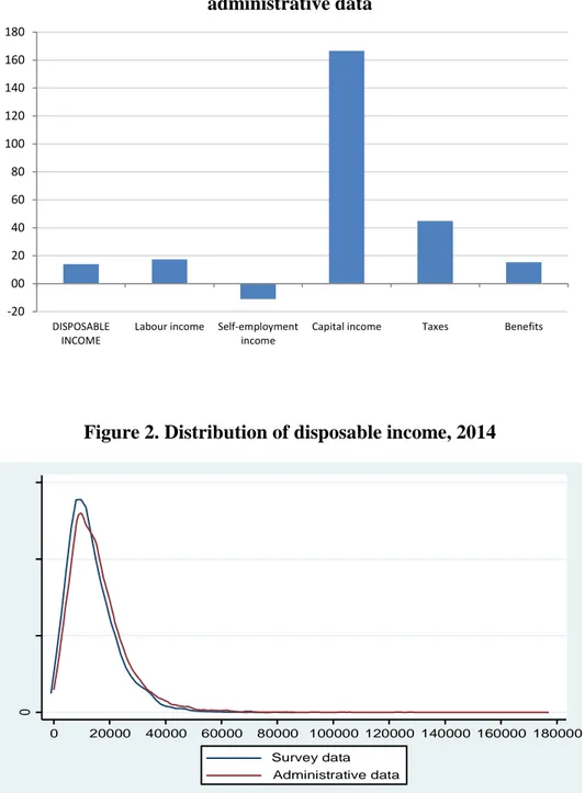
FIGURE 1
Figure 1 shows the change that occurs in the average levels of disposable income and its
different components when going from a criterion for measuring income through the
traditional method to administrative records.5 All the variations are significant and, except
in the case of self-employment income, there is an increase when going from interview
to administrative data. In line with what was anticipated by the INE, the first relevant
result is the increase in disposable income (higher than 14%).6
This growth is mainly explained by higher levels of labor income – given their weight in
total income – which grows more than 17%, and capital incomes, which are more than
2.5 times higher in administrative than in survey data. The latter is undoubtedly the source
where there is greater discrepancy between the two types of income data. The best
coverage of capital income with administrative data is an important advance in an income
source for which underreporting has traditionally been very large. The opposite occurs
with self-employment income which decreases more than 10% in administrative as
compared to survey data.
Especially relevant is the difference that may exist in the components of income related
to thepublic sector intervention, given the universal nature of administrative records. The
conversion of gross to net income is in fact a common problem in income surveys. Many
4 In the sake of simplicity we have grouped taxes and social contributions into a single category. 5 We adjust incomes using the OECD modified equivalence scale.
6 This result is very similar to that of Goerlich (2019), who finds that administrative data raised income by
10
surveys do not contain raw data and it is necessary to use algorithms for the conversion
of the net data to gross, being difficult to collect all the complexity of the tax-benefit
systems for the different individuals that make up a household (Immervoll and
O'Donoghue, 2003). The INE points out that although in the fieldwork the gross and net
level are requested for each source of income, the ignorance that in many cases the
informants have on gross income makes it necessary to construct a model that allows the
conversion of gross to net in each type of income (Méndez, 2007). As stressed by some
authors, these algorithms can affect the distributional outcomes (Goerlich, 2016). The
change from survey to administrative data increases the average level of income for cash
benefits by 15.4%. The change in average taxes and social contributions is much more
marked (around 50%). Again, this difference can decisively affect the measurement of
the redistributive effects of taxes.
3. DETERMINANTS OF INCOME UNDERREPORTING IN SURVEY DATA
The change from survey to administrative data can have important effects on the
measurement of the economic well-being of households. Opting for one procedure or
another may produce changes in the relative situation of each type of household in the
distribution of income. It may be relevant, therefore, to identify in which categories of
the population the change in income is more important when moving to administrative
records. However, the INE does not collect the survey and administrative data in the same
file. It provides different files for each type of data with different household identification
numbers in each file. In order to identify the characteristics of households and individuals
that determine a greater difference between the two types of data, it was necessary to
merge the two surveys. The objective was to obtain a single file from the resulting
matching with the different income variables with the two methodologies for the same
households. We used matching methods drawing information from the different files
provided by the INE.7
Once the matching was completed – and it was verified that the same differences in the
average levels of income sources estimated in the previous section were maintained – it
was possible to analyze in which socioeconomic categories the change of criterion has
7 Less than 5% of the observations remained unmatched and the randomization tests did not detect any
11
greater incidence. To identify the specific effect of each characteristic we estimate a
Probit model, in which the dependent variable is having an income difference higher than
the average for the whole population when moving from survey to administrative data.
We have defined this binary variable in three ways:
pi = 1 if (yAi - ySi) > (yA - yS) and pi = 0 otherwise
pi = 1 if (yAi - ySi) > 1.5 (yA - yS) and pi = 0 otherwise
pi = 1 if (yAi - ySi) > 2 (yA - yS) and pi = 0 otherwise
where yA is disposable income with administrative data, yS is disposable income with
survey data, and (yA-yS) is the average difference in disposable income with
administrative and survey data. Differences are calculated as percentages.
TABLE 1
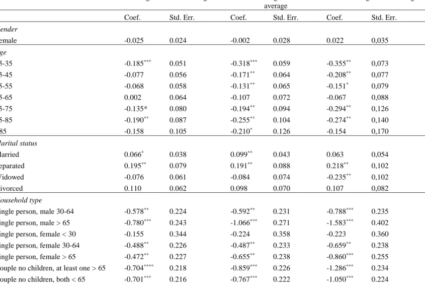
Table 1 shows the results of the estimated model. Some characteristics seem not too much
relevant to explain changes in income levels, such as gender, marital status, housing
tenure, and educational attainment. In the latter case, only the coefficient corresponding
to the individuals with the highest level is significant once the rest of the characteristics
are controlled. This result may be related, as it will be seen, with a larger income
difference in households in the upper percentiles among which there is a much higher
presence of graduates than in the lower deciles.
The results also show that when age increases – especially in individuals over 65 years of
age – the income growth when moving to administrative data is lower. This result is
related to the fact that the income of this group is largely dependent on social benefits. As
noted in the previous section, the difference in the values of benefits is small in relation
to other income sources. The different types of household generally have significant
coefficients, being lower in households with dependent children than in single persons.
Single parenthood does not appear as a characteristic associated with greater
12
One of the categories where we do find a higher likelihood of income changes when
moving to administrative data is that of immigrants from outside the European Union.
The stricter the criterion for defining that probability – a difference in income well above
the average – the more important the effect. Among the individuals who are working, the
impact of the change in the income collection method is much lower than in the rest of
the population. This result is related to the lower variation observed in labor income with
both methods. The same happens with retired people for the reasons already mentioned.
The opposite case is that of the unemployed, which seems to indicate a marked
underreporting of income from unemployment benefits when they are collected through
interviews.
4. EFFECTS ON INEQUALITY
One of the most important consequences of the change in the method to collect income is
the possible effect it can have on inequality. To the extent that the change to
administrative data produces a better reporting of some incomes – especially some of the
most unequal such as capital income – the change in method could affect the measurement
of inequality.
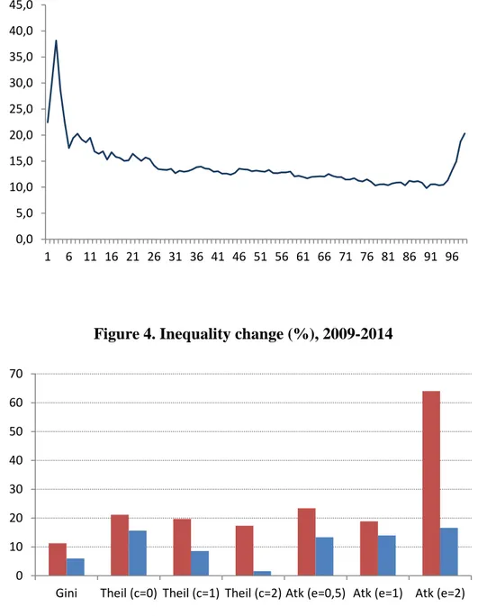
A first approach to this possible effect on inequality is the comparison of the density
functions of disposable income with the two types of data. Figure 2 shows the two
distributions for the year 2014, the last one for which comparison is possible. The data
reveal that changing to administrative data produces a shift to the right of the distribution,
a reduction in the number of households with incomes close to the modal value, and a
considerable stretch of the distribution in its upper tail. While in the survey data about
5% of households have an equivalent income around 30,000 euros, that percentage rises
to almost 8% with administrative data. There is also a greater presence of low-income
households in the distribution resulting from survey data, with 18% of households with
less than 6,000 euros, a percentage significantly higher than the one resulting from
administrative data (13%).
13
The way in which the change in methodology affects different parts of the distribution of
disposable income is best appreciated when differences by percentiles are estimated.
Figure 3 shows the growth in the average income of each percentile in percentage terms.
A first result is that administrative data increase the level of income in the whole
distribution (higher than 10% in all percentiles). A second result is that this growth is not
uniform throughout the distribution. It is especially marked in the first percentiles where
income grows more than 20%. Moreover, between the poorest 5% and the richest 5%
there is a clear decreasing profile to regrow in the higher income stratum, with income
increases higher than 15% in the richest percentiles.
FIGURE 3
Given this effect in the different sections of the distribution, the result should therefore
be a reduction in inequality when moving to administrative data. The reason is the higher
increase in income in the lower percentiles – more likely to underreport their real income
in the survey – although possibly smoothed by the growth also recorded by the richest
percentiles. In the latter case, it is easy to interpret that this growth occurs thanks to a
better coverage of capital income.
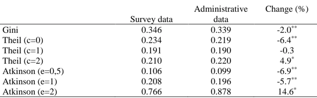
Table 2 shows a wide variety of inequality measures estimated with the two income
distributions that result from the double criterion in the collection of income. In general,
the differences for most indicators are small but significant. This is the case of the Gini
index, which modestly decreases when moving to administrative data. This result is not
repeated in all measures, which in some cases increase when moving to administrative
data.
TABLE 2
This variety of results is related to the different interpretations of inequality that each
index summarizes and to the difference in the incidence of the change in both tails of the
distribution. In the case of the Theil index,
14
Theil (1)=(1/n) in(yi/)log(yi/), c=1
Theil (0)=(1/n) log(/yi), c=0
the differences between the result with c=0 (mean logarithmic deviation) and c=2 (half
the coefficient of variation squared) are clearly related to the changes shown in Figure 3.
When c=0, the index weighs more the differences between incomes in the lower tail of
the distribution, and a very marked growth was observed in the lower income percentiles.
When c=2, changes in the upper tail of the distribution receive more weighting. As shown
in Figure 3, the change in methodology also produces a growth in the higher income
percentiles although lower than that of the other tail of the distribution. When the changes
are weighted equally throughout the distribution (c = 1), the change in inequality is very
modest and insignificant.
Something similar happens when estimating the family of Atkinson indices giving
different values to the parameter e:
Atk (e)=1-(1/n) in(yi/)1-e1/(1-e), e0 , e1
Atk (e)=1-exp(1/n) inLn(yi/)e, e=1
As this parameter grows, more weight is given to income transfers at the lower tail of the
distribution and less to those at the upper tail. This greater sensitivity to what happens in
the upper part of the distribution means that when taking high values of the parameter
(e=2) the result is a very large increase in inequality with administrative data. By contrast,
when low values are taken (e = 0.5) inequality decreases.
The availability of different ECV waves with administrative data and with the traditional
interview method allows us to assess not only how inequality changes in a given year, but
also what differences there are in the trend of inequality. The two types of distributions
can be analyzed between 2009 – the first year with administrative microdata – and 2014
– the last date in which the INE continued to collect income through the interview method.
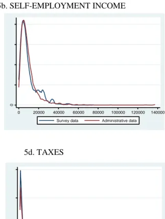
FIGURE 4
The period for which data exist corresponds to part of the most critical phase of the last
15
fell in real terms by more than 11%. In the same period, the unemployment rate raised
from 18% to 24% (Labour Force Survey). Figure 4 shows that, regardless of the indicator
chosen to measure inequality and the income data source, inequality increased during the
period considered. This growth is particularly noteworthy in the Atkinson index with the
highest parameter of aversion to inequality (e = 2) and can be also appreciated in the Gini
index.
A second relevant result – common in the set of estimated indicators – is that the growth
of inequality during this period is considerably greater when using interview than
administrative information. Thus, while the rate of growth of the Gini index during the
years considered is 6% with administrative data, it is almost double (11.3%) with survey
data. Something similar happens with the Theil (c=1) or the Atkinson (e=0.5). The widest
differences arise with the Atkinson index (e=2) and the Theil (c=2), that is, with the
indicators most sensitive to aversion to inequality and to changes in the upper tail of the
distribution. It follows therefore that one of the most important consequences of the
change in the income collection method is a smaller increase in inequality with
administrative with respect to survey data.
5. EFFECTS ON INEQUALITY BY INCOME SOURCES
The replacement of income data collected by interviews with administrative data can
affect the estimated levels of inequality through different channels. One of the most direct
is through the different impact that the change in each income source may have had on
income percentiles. Although in some of the main income sources the changes seem
relatively modest on average, it is possible that the dispersion in their corresponding
distributions changes when moving to administrative data. In the case of capital income
or taxes and social contributions, the magnitude of the difference observed with the two
criteria of income collection makes it easy to predict also a very different magnitude of
inequality in each source.
The better coverage of capital income could be determinant of an inequality level in
disposable income different from that which results from the traditional method of
collecting income. Some recent studies have emphasized the role that the increase in the
16
income (Milanovic, 2017; Bengtsson and Waldenström, 2018). A better coverage of these
incomes should also imply a different level of inequality in their distribution and the same
could happen with other sources of household income.
FIGURE 5
Figure 5a shows the density functions of labor income in each household with the two
criteria for collecting income. Although the difference in average labor income when
changing criteria was relatively small (17.4%) compared to other sources of income, some
significant changes come up in the two resulting distributions. One of the most prominent
is some displacement to the left of the labor income distribution with administrative
records, indicative of a greater number of low-wage earners with this criterion. Second,
the bimodal profile of the distribution with administrative data stands out, with the first
of these values probably reflecting earnings corresponding to part-time employment. The
highest modal value in the case of labor income with survey data evidences the greatest
weight in the distribution of average wages. Finally, as in the case of the net disposable
income, administrative data have greater coverage of high-wage workers.
The differences are much less marked in the densities of the self-employment income
(Figure 5b). The profile of the two distributions is very similar, with the only nuance of
the slightly more inward shape of these incomes with survey data in the decreasing section
from the modal value. Noticeably, these incomes are usually underreported in the
household surveys, but, at the same time, they receive in Spain a specific treatment in the
personal income tax, which means that, in many cases, the taxable income differs
markedly from the income actually received. This is the only case in which the average
income is lower with administrative than survey data. This difference between the two
types of variables occurs, above all, in the section between 18,000 and 30,000 euros,
always in terms of equivalent income. This gap is also observed in higher incomes until
the upper tail of the distribution begins to stretch, given the better coverage of the highest
self-employment incomes in administrative data.
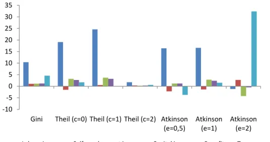
Regarding capital income, we have already noticed that this is the income source with the
highest change in mean from survey to administrative data. Moreover, as Figure 5c
17
the distribution with survey than with administrative data. The average and maximum
values of this source are very different in each case, almost doubling that of the data
obtained through interviews.
The distributions of the taxes variable do not differ substantially with the two
methodologies (Figure 5d). The large increase in the average value of taxes when these
are collected with data from the Tax Agency is mainly concentrated in the largest number
of households that now happens to be in the income bracket between 5,000 and 12,000
euros. The distribution moves to the right when moving from survey to administrative
data, and there is also a greater concentration of taxes paid around the modal value of
survey data.
Finally, cash benefits present a somewhat different profile to the previous ones (Figure
5e). In both distributions there is a greater concentration of this type of income around
low values. However, although the difference is small, there are two characteristics that
make the corresponding densities somewhat different. First, although the modal value
with interview and administrative data is similar, the number of households accumulated
around this value is clearly lower with administrative data. Second, from this value there
is a greater number of households for each income level in the case of administrative data
except in the far right of the distribution, collecting the survey data unusually high
benefits.
The different shapes observed in the distributions of each income source allow us to
anticipate that the indicators that summarize inequality in each case will differ as
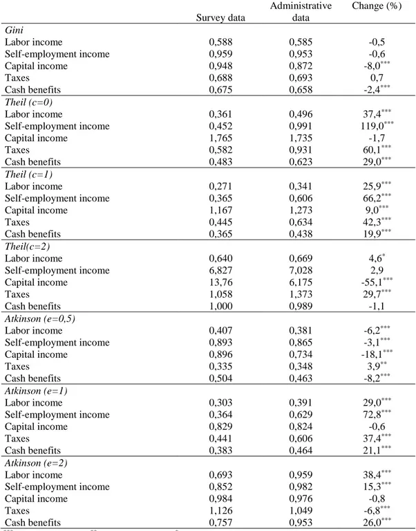
measured by the traditional method of interview or using administrative data. Table 3
shows these indicators and the difference between the two methods, also indicating the
statistical significance of the latter. A first result is the different sign and significance of
the Gini index by income sources, as compared to other inequality indexes. In particular,
according to Gini index, in most income sources the methodological change gives rise to
a more equal distribution, although the differences – except in capital income and cash
benefits – are not significant. The only exception is taxes, whose internal inequality must
be interpreted inversely to the other sources. The different results for the Gini index could
be explained – as it was deduced from the analysis of the density functions of each source
18
administrative data are much larger in the tails of each distribution than in middle
incomes.
TABLE 3
This result is also found with the Atkinson index with the parameter that represents a
lower aversion to inequality, but not with the Theil index when all incomes receive a
similar weighting. It is precisely in this indicator that the effect of the methodological
change on inequality in all income sources is larger.
Among the different income sources analyzed, the most important changes are those
affecting capital and self-employment income, being smaller – although depending on
each indicator – the changes in the inequality of labor income. Given the greater weight
of the latter on total household income, it is normal that the effect on inequality of
disposable income is small in most of the indicators. On the other hand, the impact of the
greater coverage of capital income produces in general a reduction in inequality in this
source. The opposite occurs with self-employment income with almost all indicators
showing higher inequality levels.
If the results corresponding to the effect of the methodological change on inequality in
the different sources are compared with the previous results on the change in their average
levels, there seems to be a certain relationship. In general terms, the income sources in
which levels change the most when modifying the method of income collection –capital
income and taxes – are also those in which moving to administrative data has the greatest
impact on inequality.
6. EFFECTS ON THE STRUCTURE OF INEQUALITY AND DEPENDENCES BETWEEN INCOME SOURCES
A very important dimension of inequality that may be affected when moving from survey
to administrative data is the structure of inequality by income sources. The inequality of
the distribution of disposable income is the result of the inequality in the different sources
of income, the weight in the total income of each source and the correlations between
19
administrative data can affect the first two components. Far less research has examined
how the different methods of collecting income can yield different results in terms of the
dependences between the income sources.
In recent years, increasingly robust procedures have been developed for the analysis of
inequality by income sources, taking into account both changes in the structure of the
population and those related to its various components. The decomposition of inequality
by income sources has as its main reference the pioneering contributions of Shorrocks
(1982, a, b). His works were based on inequality at a fixed moment in time. Jenkins (1995)
generalized this analysis to decompose trends.
Recent studies have expanded the decomposition method through two extensions. One
has been to consider a wider variety of inequality indicators, and another one is the
combination in a single method of analysis of changes in individual characteristics and
changes in income sources and their dependences. The pioneering contribution was
Dinardo et al. (1996), which was further developed in the field of inequality of disposable
income by Daly and Valleta (2006). It is a structural method, in which the contribution of
each component is identified through a counterfactual. They compare the distribution
with the observable characteristics in the present moment and the one that would exist if
those characteristics had not changed over time. The major criticism that this approach
has received is that the results can be very sensitive to the specification of the model
(Cowell and Fiorio, 2011), being also a very limited approximation to identify the
interrelations between income sources.
In our specific case, the analysis is markedly simplified because – being the same
individuals and households –, there is no change in the characteristics and we can focus
on the other two types of effects. In our approach to the change produced by the
administrative data in the structure of inequality, we will combine two type of analysis
that try to overcome the limits of the cited approaches. First, as proposed by Larrimore
(2004), we create a counterfactual that maintains the order of the initial distribution of
income – survey data – to determine how the changes in the marginal distributions of
each income source, when moving to administrative data, affect the differences in the
distribution of disposable income. The main limitation of this approach is that it does not
20
reason, in a second analysis we evaluate the change in dependences between income
sources through copula functions.
Let X(i) denote the total income of individual i in the initial distribution with survey data
and let us assume that it can be represented as the sum of the incomes obtained from each
source, fki, with k=1,…,d, i.e.
X(i) = f1i + f2i +…+ fdi
To estimate the impact of the change in the distribution of the first income source on the
inequality in disposable income, the income of that source with survey data ( f1i ) can be
replaced for each individual by the income of that same source with administrative data
(f’1i ), that is:
X(i)’ = f’
1i + f2i +…+ fdi
The difference between the inequality with the initial distribution and this simulated
distributioncan be interpreted as the contribution of each source to inequality. However,
the sum of these contributions is not 100%, since we should add the effect of the
dependences between income sources.
FIGURE 6
Figure 6 shows the change in the contribution to inequality in disposable income when
replacing survey by administrative data in the different sources. The contribution of each
source varies according to the indicator taken as a reference. Except in the case of the
Atkinson Index with e=2, in all other indices the greatest change in the contribution to
inequality is that of labor income. With that index, taxes are the source with the largest
change in its contribution to inequality. In any case, this latter effect is largely dependent
on inequality aversion. The impact of replacing taxes with administrative data has a
negative effect on inequality with parameters of aversion less than 1, and the impact is
21
The effects of capital income are similar in terms of the sign – although with different
size – to those of labor income. In almost all indices, the shift from survey to
administrative data noticeably increases the contribution of labor income to inequality,
except in the case again of the Atkinson Index with the highest aversion to inequality.
The effect of the changes in benefits and self-employment income are not very relevant
in quantitative terms.
A last and very important dimension of inequality that could be affected by the change of
criteria in the method for collecting income data is the structure of dependences between
income sources. As mentioned above, inequality in disposable income is the result of the
inequality in the different income sources, the relative weight of each source in total
income, and the interactions between them. Therefore, a key issue is identifying, as
accurately as possible, the effect on the dependences between income sources. However,
this issue is often forgotten. In this paper, we address the problem of both measuring the
dependence between the different income sources and analyzing whether using
administrative or survey data could affect such dependence. As this is a multidimensional
problem with more than two variables involved and those variables are non-normally
distributed, we need measures of dependence that capture other types of relationships
beyond linear correlation.
In this setting, copulas become an essential tool, as they enable building scaled-free
measures of multivariate dependence that generalize some well-known coefficients of
association like the Spearman's rho. Since there are few applications of this approach in
welfare economics (see Decancq (2014) and Pérez and Prieto (2015, 2016a)), we first
review some preliminary results concerning copulas and dependence.
A d-dimensional copula is a multivariate distribution function C:Id → I, whose
one-dimensional margins are uniform on I, where I = [0,1]. The Sklar’s theorem ensures that
given d continuous random variables, X=(X1,…,Xd), with joint cumulative distribution
function F and marginals F1,…,Fd, respectively, there exist a unique copula C such that
22
Hence, for a given real vector u = (u1,…,ud) Id, the value C(u) represents the proportion
of individuals in the population with positions outranked by u – i.e., with a lower or equal
position than u in all dimensions. For instance, C(0.1,…,0.1) will represent the probability
that a randomly selected individual is simultaneously in the first decile (“low ranked”) in
all dimensions. By contrast, the survival function 𝐶̅ associated with the copula C, is
defined as
𝐶̅(u) = p(U1 > u1,….,Ud> ud),
where Ui=Fi(Xi), i=1,…,d, are uniform U(0,1) random variables with joint distribution C.
Hence, the function 𝐶̅ represents the proportion of individuals in the population with
positions higher than u in all dimensions. That is, 𝐶̅(0.9,…,0.9) will represent the
probability that a randomly selected individual is simultaneously in the 9th decile (“top
ranked”) in all dimensions. In general, 𝐶̅ is not a copula. If the variables X1,..,Xd are
independent, their copula will be the independent copula Π, defined as Π(u)=u1.ud.
The essential feature of the copula approach is that it allows us to decompose the joint
distribution of X into their one-dimensional marginal distribution functions and the
dependence structure between them, which is captured by the copula, as stated in 1. In
terms of the discussion on the possible effects of the different methods of data collection,
the key question is whether this dependence differs with the two types of data. Given that
we deal with five income sources, measures of multivariate dependence are needed to test
whether the two types of data yield similar results in terms of the relationships between
the different sources.
There are several copula-based measures of multivariate dependence proposed in the
literature (see Schmid et al. (2010)). In this paper, we focus on three multivariate
extensions of the bivariate Spearman’s rho based on orthant dependence concepts.
Roughly speaking, measuring lower (upper) orthant dependence amounts to compare how
likely it is that the variables X1,…,Xd take simultaneously small (large) values as
compared to how likely this would be were the variables independent.8
23
The first copula-based multivariate extension of Spearman’s rho we consider is due to
Wolff (1980) and Nelsen (1996) and it is defined as follows:
𝜌d− = (𝑑+1)
2𝑑−(𝑑+1)∫ [𝐶(𝒖) − 𝛱(𝒖)]d𝒖𝑰𝑑 . 2
Hence, 𝜌d− can be regarded as a measure of average lower orthant dependence, as it
measures, to some extent, the rescaled “average distance” between our multivariate data
(represented by its copula C) and independence (copula ) in the lower orthant.
In a similar fashion, Nelsen (1996) defined a measure 𝜌d+ of average upper orthant
dependence as follows:
𝜌d+ = (𝑑+1)
2𝑑−(𝑑+1)∫ [𝐶̅(𝒖) − 𝛱𝑰𝑑 ̅(𝒖)]d𝒖 3
This measure can be regarded as a rescaled “average distance” between C̅ – representing
the behaviour of our data in the upper orthant – and Π̅ – representing independence in
such orthant.
The third multivariate version of Spearman’s rho, due to Nelsen (2002), is the average of
the two generalizations described above, namely:
𝜌𝑑 = 1 2(𝜌𝑑
−+ 𝜌
𝑑+) 4
Positive values of the three coefficients in [2]-[4] indicate positive lower orthant, upper
orthant and orthant dependence, respectively. Furthermore, when the components of X
are independent (C=), the three coefficients become zero, whereas in the case of
maximal dependence, i.e. the outcomes in all the variables X1,…,Xd are ordered in the
same way, they all reach their maximum value, 1. A lower bound for the three of them is
[2d – (d + 1)!]/{d![2d – (d + 1)]}; see Nelsen (1996). For our purposes, the coefficients 𝜌𝑑−
and 𝜌d+ are preferable, as they can reveal some forms of dependences that 𝜌𝑑 fails to
detect; see Example 2 in Nelsen (1996). Noticeably, in the bivariate case (d=2), the three
24
copula C is unknown and the coefficients in [2]-[4] must be estimated from the data by
using the empirical copula. Pérez and Prieto-Alaiz (2016b) propose feasible
nonparametric estimators of 𝜌𝑑− and 𝜌𝑑+ that are easy to compute and share good
asymptotic properties. The average of these estimators could be used to estimate 𝜌𝑑.
The discussion so far is based on the assumption that the univariate margins are
continuous. Without this assumption, the underlying copula C in (1) is no longer unique,
although it is uniquely determined on RanF1 … RanFd. Accordingly, the coefficients
in equations 2-4 should be modified when dealing with possibly non-continuous
random variables; see, for instance, the proposals in Quessy (2009) and Mesfioui and
Quessy (2010) and their corresponding estimators in Genest et al. (2013).
Next, we apply the measures discussed above to the analysis of the dependence between
the different income sources in order to check whether the degree of dependence change
depending on the type of data used. To ease the computation and interpretation of the
results, the income sources have been aggregated into three components (d=3): labor
income (labor income plus self-employment income), capital income and the net results
of taxes and transfers (taxes minus cash transfers). Since our variables are not strictly
continuous, to compute the empirical versions of the coefficients 2-4, we use the
estimators proposed by Genest et al. (2013) for d=3. In order to compute the standard
errors of these estimators, we approximate their bootstrap distribution by resampling with
replacement repeatedly from the original data (1,000 subsamples). Then, on the basis of
the bootstrap distributions obtained, we test whether the difference between survey and
administrative data is significant. Table 4 depicts the results.
TABLE 4
Several conclusions emerge from this table. First, regardless of the coefficient used, there
is a positive and significant multivariate dependence between the income sources, both in
survey and administrative data. Second, regardless the data source, the largest coefficient
of multivariate dependence is 𝜌𝑑+. This means that high values of the three income
components tend to occur together – i.e., people with high labor income are more likely
25
simultaneous occurrence of “good” rankings in the three components is more likely with
administrative than with survey data. By contrast, the coefficient 𝜌𝑑− is significantly
greater with survey than with administrative data. This means that small levels of the
three income components (labor, capital, tax-public transfers) tend to occur together more
likely with survey than with administrative data. Noticeable, there is no significant
difference between the coefficient with the two types of data. This results underlines
the caveats of only using this coefficient since, as commented before, it could mask some
type of dependences that are only captured by 𝜌𝑑− and 𝜌𝑑+.
In general terms, it can be said that both methods of data collection also produce
significant differences in the observed dependences between income sources. Therefore,
moving from one method to another affects not only the level of inequality and its changes
over time, but also the very structure of inequality.
7. CONCLUSIONS
The past decade has witnessed an intense debate over the trends and consequences of
inequality. The importance of its analysis requires having robust datasets to understand
its changes, determinants and implications. Almost all countries have datasets that allow
for a sufficiently comprehensive picture of the evolution of inequality in the long term.
In most cases, these are household surveys that provide detailed data on the different
income sources that each individual receives. However, survey income data are affected
by different types of problems – non-response, measurement error, limited representation
of top incomes – that may limit their ability to provide accurate diagnoses for decision
making.
Due to these limitations, some countries are replacing in the surveys the income data
collected through interviews by administrative data. Such a process can have important
effects on the measurement of inequality and, therefore, on the optimal design of
redistributive policies. It is necessary to evaluate not only how it affects the general
indicators but also the inequality by income sources and the structure of dependences
26
The change in the method of income collection in the main household survey in Spain
(ECV) – moving from survey to administrative data – has made it possible to evaluate the
possible impact that this type of changes has on income inequality and its structure. A
great advantage compared to previous studies is that both types of data are available
simultaneously for the same individuals and households. In this paper we have reviewed
in depth some of the effects that this methodological change has had on inequality and its
structure by income sources.
The general result is that moving to administrative data has effects on the levels of the
different income variables included in the survey, the magnitude of inequality in the
distribution of income, and its structure by income sources. Our analysis confirms, first,
a significant growth of household disposable income with administrative data. This
increase is especially important in capital income, with a notable improvement in a source
where levels of under-reporting in survey data are usually very high. The opposite occurs
in self-employment income, reflecting the comparison between survey and tax data the
special treatment these incomes receive in the personal income tax.
A second contribution has been to identify the population categories that show greater
differences depending on the method of income collecting. While there are some little
differentiating characteristics – gender, marital status or educational level – there are
others associated with a higher probability of income under-reporting in surveys. This is
the case, among others, of age, the type of household, nationality, and unemployment
status, for which the administrative data substantially correct the lack of coverage of the
surveys.
One of the fundamental questions that the paper addresses is whether the change in the
method of income collection affects the measurement of inequality. It can be stated that
the difference in income according to one or another criterion is not independent of the
level of household income. The incomes of the tails of the distribution increase
considerably more – especially in the lower part of the distribution – than those of the
middle strata. On the other hand, inequality indicators are significantly lower with
administrative data. This result is reversed only in those indicators assigning much more
27
A fourth contribution is the identification of those income sources that are most sensitive
to the use of administrative data in terms of their corresponding inequality levels. Turning
to administrative data generally leads to more equal distributions in each income source.
One of the most relevant effects of using administrative data is the modification of the
structure of inequality, rising above all the contribution of capital income, cash benefits
and taxes.
Lastly, we have shown that there are also significant differences in the structure of
dependence between income sources depending on which income data source we use. In
particular, moving from survey to administrative data conveys both a significant increase
in the upper orthant dependence and a significant decrease in the lower orthant
dependence. This is a key issue in the design of optimal redistributive policies, as it affects
28
References
Alvaredo, F., Atkinson, A.B., Piketty, T. and Saez, E. (2015): The World Top Incomes Database,
http://g-mond.parisschoolofeconomics.eu/topincomes.
Atkinson, A.B. (2015): Inequality. Cambridge, Ma: Harvard University Press.
Atkinson, A.B. and Piketty, T. (2010): Top Incomes: A Global Perspective. Oxford University Press.
Auten, G. and Splinter, D. (2019): “Top 1 Percent Income Shares: Comparing Estimates Using Tax Data”. AEA Papers and Proceedings 109, 307–311.
Bengtsson, E. and Waldenström, D. (2018): “Capital Shares and Income inequality: Evidence from the Long Run”. The Journal of Economic History 78, 712-743.
Burkhauser, R.V., Feng, S., Jenkins, S.P. and Larrimore, J. (2012): “Recent Trends in Top Income Shares in the United States: Reconciling Estimates from March CPS and IRS Tax Return Data”.
The Review of Economics and Statistics 94, 371-388.
Burkhauser, R.V., Hérault, N., Jenkins, S.P. and Wilkins, R. (2016): “What Has Been Happening to UK Income Inequality since the Mid-1990s? Answers from Reconciled and Combined Household Survey and Tax Return Data”. IZA Discussion Paper 9718.
Carr, M.D, and Wiemers, E.E. (2018): “New Evidence on Earnings Volatility in Survey and Administrative Data”. American Economic Review: Papers and Proceedings, 108, 287-291.
Courtemanche, C, Denteh, A, and Tchernis, R. (2019): “Estimating the Associations between SNAP and Food Insecurity, Obesity, and Food Purchases with Imperfect Administrative Measures of Participation”. Southern Economic Journal (forthcoming).
Cowell, F. and C.V. Fiorio (2011): “Inequality Decompositions—A Reconciliation”. Journal of Economic Inequality 9, 509-28.
Dahl, M., DeLeire, T., and Schwabish, J.A. (2011): “Estimates of Year-to-Year Volatility in Earnings and in Household Incomes from Administrative, Survey, and Matched Data”. The Journal of Human Resources 46, 750-774.
Daly, M. C. and Valletta, R.G. (2006): “Inequality and Poverty in the United States: The Effects of Rising Dispersion of Men’s Earnings and Changing Family Behavior”, Economica 73, 75-98.
Decancq, K. (2014): “Copula-based measurement of dependence between dimensions of wellbeing”. Oxford Economic Papers, 66(3), 681-701.
DiNardo, J. E., N. Fortin, and Lemieux, T. (1996): “Labor Market Institutions and the Distribution of Wages, 1973–1992: A Semi-Parametric Approach,” Econometrica, 64, 1001-44.
Genest, C., Nelšehová, J., and Rémillard, B. (2013): “On the estimation of Spearman’s rho and related tests of independence for possibly discontinuous multivariate data”,
Journal of Multivariate Analysis, 117, 214-228.
Goerlich, F.J. (2016): Distribución de la renta, crisis económica y políticas redistributivas.
29
Goerlich, F.J. (2019): “Las mil caras de la desigualdad y una más: La obtención de los ingresos en la Encuesta de Condiciones de Vida” (mimeo)
Higgins, S., Lustig,N. and Vigorito, A. (2018): “The rich underreport their income: Assessing bias in inequality estimates and correction methods using linked survey and tax data”. ECINEQ WP 2018 – 475.
Immervoll, H. and O'Donoghue, C. (2003): "Imputation of Gross Amounts from Net Incomes in Household Surveys. An Application using EUROMOD," Computational Economics 0302001, EconWPA.
INE (2010): “Oportunidades de aprovechamiento de registros administrativos en la ECV. Análisis realizado con la encuesta 2007”. INE (mimeo).
INE (2014): “Aprovechamiento de los ficheros administrativos en la Encuesta de Condiciones de Vida”. Madrid: Instituto Nacional de Estadística.
Jenkins, S. P. (1995). “Accounting for inequality trends: Decomposition analyses for the UK”.
Economica 62, 29-64.
Kyzyma, I., Fusco, A. and Van Kerm, P. (2014): “Accounting for changes in the distribution of household income by its sources: Decomposition based on copula function”. Paper presented at IARIW 33rd General Conference. Rotterdam, August 24-30, 2014.
Larrimore, J. (2014): “Accounting for United States Household Income Inequality Trends: The Changing Importance of Household Structure and Male and Female Labor Earnings Inequality”.
Review of Income and Wealth 60, 683–701.
Lynn, P., Jäckle, A., Jenkins, S.P., and Sala, E (2012): “The impact of questioning method on measurement error in panel survey measures of benefit receipt: evidence from a validation study,”
Journal of the Royal Statistical Society, Series A 175, 289–308.
Méndez, J.M. (2007): “Oportunidades en el uso de registros administrativos en la Encuesta de Condiciones de Vida y en la Encuesta Continua de Presupuestos Familiares”. En Marcos, C. (coord..): El papel de los registros administrativos en el análisis social y económico y el desarrollo del sistema estadístico. Madrid: Instituto de Estudios Fiscales.
Méndez, J.M. and Vega, P. (2011): “Linking data from administrative records and the Living Conditions Survey”. INE Working Papers 01/2011.
Mesfioui, M. and Quessy, J.-F. (2010): “Concordance measures for multivariate non-continuous random vectors”, Journal of Multivariate Analysis, 101(10), 2398-2410.
Meyer, B.D., Mok, W. and Sullivan, J. (2015): “Household Surveys in Crisis”. Journal of Economic Perspectives 29, 199-226.
Meyer, B.D. and Mittag, N. (2019a): “An Empirical Total Survey Error Decomposition Using Data Combination.” IZA Discussion Paper 12151.
Meyer, B.D. and Mittag, N. (2019b): “Combining Administrative and Survey Data to Improve Income Measurement,” IZA DP No. 12266.