Distributions of city sizes in Mexico during the 20th century

(1)

Distributions of city sizes in Mexico during the 20th century

Enrique Pérez-Campuzano

a

, Lev Guzmán-Vargas

b,⇑

, F. Angulo-Brown

c

a_{Instituto de Geografía, Circuito Exterior, Col. Universidad Nacional Autónoma de México, UNAM, México D.F. 04510, Mexico} b

Unidad Profesional interdisciplinaria en Ingeniería y Tecnologías Avanzadas, Instituto Politécnico Nacional, Av. IPN No. 2580, México D.F. 07340, Mexico c

Departamento de Física, Escuela Superior de Física y Matemáticas, Instituto Politécnico Nacional, Edif. No. 9 U.P. Zacatenco, México D.F. 07738, Mexico

a r t i c l e

i n f o

Article history:

Received 19 November 2014 Accepted 19 December 2014 Available online 21 January 2015

a b s t r a c t

We present a study of the distribution of cities in Mexico along the 20th century, based on information collected in censuses every ten years. The size-rank and survival cumulative distributions are constructed to evaluate the presence of scaling, its deviation from the Zipf’s law and their evolution along the period of observation. We ﬁnd that the size of cities

S, approximately follow a power-law with the rankr;SðrÞ ra_{, where the exponents take}

values betweena0:7 toa1:1 for years 1900 and 2000, respectively. The local fluctu-ations in the scaling behavior are evaluated by means of a local exponent, and the deviation of the size predicted by the Zipf’s law (a¼1) and the real size of each city is analyzed. Our calculations show that local exponents follow transitions between values above and below of the Zipfian regime and the deviations are more remarkable at the beginning and at the end of the 20th century. Besides, the cumulative distributions confirm the presence of scal-ing for the same records with a reasonable agreement with the scalscal-ing exponents observed in the size-rank distributions. Moreover, we examine the role of a recent introduced prop-erty named coherence. Finally, we explain our findings in terms of the socio-demographic evolution of Mexico along the 20th century.

1. Introduction

Since Pareto[1]in the 19th century up to the present

day, many complex collective phenomena have been sta-tistically described by scaling laws. This approach has been used in a variety of research ﬁelds ranging from social to

natural sciences[2]. For example, from economics[3–5],

linguistics[6,7] and sociology[8] to physics [9–11]and

biology [12]. The phenomena described by scaling laws

have no characteristic scales and usually are described by power laws of the fractal type. Scaling relationships were ﬁrst found on empirical grounds. A clear case of this is that of the empirical laws of seismology, such as the so-called

Omori law for aftershocks temporal distribution[13] or

the Gutenberg–Richter law for the magnitude distribution

of seisms [14]. Several decades after these laws were

established empirically, Bak et al.[15,16]proposed a more

fundamental explanation for them based on the concept of self-organized critical systems. The same happened with the scaling laws of the Zipf type, followed by the

distribu-tion of cities by size [17], which were ﬁrst empirically

established and until recent times more detailed

mecha-nisms for their explanation have been proposed [18,19].

On the other hand, as it is well known, only the self-similar fractals, as the Koch’s curve for instance, have scaling laws over an arbitrary number of scales. However, the scaling properties in real world objects and phenomena are incomplete in the sense that the corresponding power laws typically have one or more crossovers in their scaling

expo-nents [20]. For example, the Gutenberg–Richter law for

earthquakes extends along many decades from millimeters up to thousands of kilometers, however, it has a crossover

⇑ Corresponding author.

E-mail addresses: eperez@igg.unam.mx (E. Pérez-Campuzano), lguzmanv@ipn.mx (L. Guzmán-Vargas), angulo@esfm.ipn.mx (F. Angulo-Brown).

Contents lists available atScienceDirect

Chaos, Solitons & Fractals

Nonlinear Science, and Nonequilibrium and Complex Phenomena

(2)

other hand, large earthquakes have no bounds in rupture length, but their down-dip width is limited by thickness

of the region capable of generating earthquakes[21].

Another case where a crossover plays a very important role is that corresponding to empirical data of distribution of the money and wealth in many countries as in UK for

example[22,23]. When a log–log plot of cumulative

prob-ability distribution against total of capital (wealth) is made, clearly two well deﬁned regions are found, one fol-lowing a Pareto-type behavior for rich people and other following an experimental distribution of the Boltzmann-type for the lower part of the distribution for the great majority (about 90%) of the population. Some

well-founded models explain these different behaviors[22,24–

26]. For the case of the city size distribution, deviations

from Zipf’s law and crossovers have been reported [27–

30]. As in the case of the money and wealth distributions,

crossovers between big (S>105 _{inhabitants) and small}

scales, and between developed and developing countries have been identiﬁed. For the case of Japan for instance, Sasaki et al. reported that the rank-size distributions of towns and villages can be well approximated by log nor-mal distributions while for cities a power-law distribution

is observed. On the other hand, Malacarne et al.[31]also

have reported that for the cases of Brazil and USA a notori-ous deviation from an asymptotic power-law of the Zipf type is found when cities of all sizes are considered. Until the present day, there is no consensus about the best ﬁt

of city size distributions. For example, Bee et al.[32]

ques-tion the claim that largest US cities are Pareto distributed and based on multiple tests on real data they assert that the distribution is lognormal, and largely depends on

sam-ple sizes. On the other hand, Giesen et al.[33]by using

un-truncated settlement size data from eight countries show that the ‘‘double Pareto lognormal’’ distribution provides a better ﬁt to actual city sizes than the simple lognormal

distribution. More recently, Cristelli et al. [27] have

reported a very important property called ‘‘coherence’’ of the sample of objects to be studied, which drives the

resulting power-law towards a perfect Zipf’s law (

a

¼1)

or towards marked deviations from it. Another important feature of city size distributions (CSD), is the time evolu-tion of the power-law exponents depending of many

social, economic and political phenomena [27,31]. The

CSD has been studied for many countries as USA ([34]),

Spain [35], France [28], Japan [28], India [36], China

[36,37], Brazil[38]among others. The study of particular cases is important because they help to enrich the phe-nomenology of the CSD problem. In the present article we study the case of Mexico by analyzing each decade cen-suses from 1900 up to 2000. The main goal of this work is to evaluate presence and departures of the scaling behav-ior in CSD, and deviations with respect to the Zipf’s regime. Our results clearly reﬂect some of the main social and eco-nomic transitions of Mexico along the 20th century under

and ﬁnally in Section 4 some concluding remarks are given.

2. Data and sociodemographic aspects

One of the big issues in the construction of the relation-ship between population and rank of cities is the deﬁnition

of a city[36]. Some authors use a spatial deﬁnition for

cit-ies, particularly based on the amount of building area.

Other studies [39] use an administrative deﬁnition, i.e.

government of specific states or cities. In the case of this study, we combine both perspectives. In first place, metro-politan zones are defined as municipalities agglomera-tions; that is, data corresponding to the total of the population of the municipalities and they were taken from

different sources[38,40,41]. We follow the common

prac-tice in Mexico to assume the size of 15 000 inhabitants as

the lower threshold to deﬁne a city[38]. Although there

are some criticisms to this threshold, it remains as the most extended deﬁnition used in Mexico (our dataset can

be freely accessed on the website http://www.cslupiita.

com.mx/citiesmx/).

Along the 20th century, as many countries in the world, Mexico passed through important transformations,

includ-ing its transition from a rural to an urban country[42]. As

can be seen inFig. 1, the annual growth rate (AGR) of the

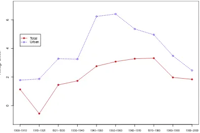
urban population was higher than the AGR of total popula-tion for the considered period. In the 1950’s the largest dif-ference between both AGR’s is observed due to the industrialization policy, the promotion of the urbanization, and rural to urban migration. Thanks to the population pol-icies since the 1970’s, it seems that nowadays both AGR’s are close each other. In 1900, just the 10.6% of the popula-tion lived in one of the 33 Mexican cities. By 2000, 364 cit-ies formed the Mexican urban system with more than 60 million inhabitants (63% of the total).

Some authors such as Unikel [38,43], Garza [40] and

Aguilar and Graizbord [42] have pointed out the

importance of dividing the recent urban history of Mexico in three periods: I. 1900–1939, II. 1940–1979 and III.

1980–2000 (seeTable 1). In 1900, Mexico was a rural

coun-try. The urban population (10.6%) was distributed in 33 cit-ies and six of them concentrated the one half of the total. During the ﬁrst period the percentage of urban population grew around 7% meanwhile the total of cities reached 43 (i.e. 30%).

In the second period (1940–1979), the process of urban-ization took place in a faster rate due to a state policy of industrialization and urbanization. By the beginning of this period, around 20% of the total of population lived in 55 cities, meanwhile by the end the urban population reached 46% and the total of cities was 167. In other words, urban population doubled meanwhile the total of cities tripled.

(3)

brought important transformations in both policy terms and spatial distribution of people. The most important is that urban population surpassed the 50% of the total. The second one is the increment in the total number of cities. By the beginning of the period, there were 220 but by the end the total reached 350. The social and economic impacts of the neoliberal policies during this period are evident. For example, the so-called macroeconomic indica-tors showed a seemingly general advancement, however, the microeconomic ones; that is, those that measure the actual economic status of the majority of population did not exhibited remarkable improvements, indeed, some of these indicators worsened.

The CSD in Mexico along the 20th century is a very interesting problem because of during this period it

evolved from a mainly rural country towards a society that behaves like a mixture of a developed and a developing country.

3. Results and discussion

Prior to describe our results, we provide a brief descrip-tion of some mathematical aspects of Zipf’s and Pareto’s distributions. Zipf’s plots or size-rank distributions have

the formSðrÞ ¼ara_{, where}_S_ð_r_Þ_and_r_{are the size in terms}

of population of the cities and the rank, respectively;a;

a

are ﬁtting parameters[2,44]. Commonly, when

a

¼1 this

relationship is referred as the Zipf’s law or Zipﬁan regime; and when the statistics is based on the probability of

hav-ing cities with sizes bigger thanS, with a functional form

given by,Pð>SÞ Sc_{, it is called Pareto’s law and}

_c

_{is an}

exponent related to the size-rank exponent through,

c

1=

a

[44]. For simplicity, in what follows, we will refer

toPð>SÞas the cumulative distribution function (CDF). To start our analysis of the sizes of cities along the 20th century, we construct the size-rank plots for each decade. Fig. 2shows the statistics of rank against the size of Mex-ican cities for ten censuses. The best ﬁt, using the ordinary least square (OLS), leads to the exponent values showed in Table 2. We observe a clear increasing tendency in the exponents as the time evolves, with values above one for recent data. Interestingly, the CSD exponents since 1900 up to 1960 had a homogeneous behavior expressed by means of practically linear ﬁttings (especially, if Mexico

City is excluded). The

a

-exponents grew from 0.76 until

1.04 during this period; that is, the

a

’s evolved from a value

corresponding to an uneven distribution of cities up to a

02

46

Average Growth

1900−1910 1910−1921 1921−1930 1930−1940 1940−1950 1950−1960 1960−1970 1970−1980 1980−1990 1990−2000

[image:3.544.80.474.53.315.2]

Total Urban

[image:3.544.41.263.396.516.2]

Fig. 1.Annual growth rates for the period 1900–2000. We show the cases of the urban (open circles) and the total (closed circles) population. It is noteworthy that the urban growth is higher that the total one.

Table 1

Main aspects of the three periods along the 20th century (see text for details). The number of cities, the increment of the total number of cities (ITC) and the urban population percentage (UPP) are listed.

Period Year Cities ITC % UPP

I. Post revolution 1900 33 – 10.6

1910 33 0 11.3

1921 37 4 14.4

1939 43 6 17.2

II. Endogenous growth 1940 55 12 20.0

1950 83 28 27.9

1960 120 37 38.3

1979 167 47 46.8

III. Neoliberal 1980 220 53 54.8

1990 306 86 63.5

(4)

more egalitarian distribution; that is, a more evenly spread of the population across the country. This global behavior from 1900 until 1960 can be interpreted within the context

of the ‘‘coherence‘‘ concept coined by Cristelli et al.[27],

which has to do with the internal consistency or complete-ness of the total sample under examination. To exemplify

this concept these authors[27]show how the frequency

of words in the Corpus of Contemporary American English displays a quasi-perfect Zipf’s law and also how the rank of the Gross Domestic Product (GDP) of world countries has a Zipfian behavior for the 30th richest. Another case of a good Zipfian fitting is that corresponding to the CSD of

Nigeria. For the GDP case, Cristelli et al.[27]interpret the

Zipﬁan behavior in terms of globalization as a mechanism of internal coherence of this system. On the other hand, for Nigeria, despite being a developing country, it has an inter-nal coherence stemming from a developing in a more uni-form, isolated and self integrated fashion. Returning to the

Mexico’s case, Fig. 2 shows how from 1960 until 2000,

despite of the

a

exponents are within the interval

½1:045;1:115, the quality of the linear ﬁtting is remarkable

deteriorated, mainly due to the growth of cities with

pop-ulation between 105and 106inhabitants; that is an

accel-erated growing of intermediate city-sizes.

As it can be seen inFig. 6, this notorious deviation is a

contribution of the northern cities located near the border

with USA[45]. Much of this phenomenon has to do with

the great economic ‘‘gradient’’ exercised by a strong econ-omy on a weak one, which is the case in the USA–Mexico interaction.

Next, we evaluate the properties of the scaling behavior

observed inFig. 2from two perspectives: (i) The

concor-dance of the global scaling exponent with the local one; and (ii) the deviation of the size predicted by the Zipf’s

law (

a

¼1) and the real size of each city. Concerning (i),

to asses the behavior of the local exponent,

a

l, along

differ-ent rank scales, we calculate this expondiffer-ent in the following way,

al

¼ dlogSðrÞ

dlogr : ð1Þ

The resulting values of

a

l as a function of the rankrare

showed inFig. 3(a). We show that the local exponent is

not stable, leading to different scaling behaviors, but the rounded crossover between different scales seems to be important when the global (over all scales) ﬁt is performed,

presenting a power law scaling of the form 1=ra_{. A more}

detailed observation of the local exponents reveals the presence of crossings between values below and above one, indicating the scales where the rank statistics deviates from the Zipﬁan regime. Regarding (ii), we use the

approach suggested by González[30]to evaluate the

devi-ation of the real city-sizeSwith respect to the one

pre-dicted by the Zipf’s law (S). The deviation is captured by

the statistics[30],

lnðS=SÞ ¼ ð1=

a

1ÞðlnrlnNÞ ð1=

a

Þ^_e; ð2Þ

100 101 102 103

Rank r

104 105 106

Size (number of citizens)

70 80 90 2000

[image:4.544.150.386.54.228.2]

slope=0.5

Fig. 2.Rank vs. size plot for cities in Mexico along the 20th century. We observe a Zipf’s distribution of the form,SðrÞ ra_{. The value of the exponent}_a

increased from 0:78 to 1:1 during the period under study, revealing changes in the city growth mechanisms. We also notice the deviations from the power-law behavior from year 1970 and up.

Table 2

Summary of scaling exponents observed in Zipf plots and cumulative distributions for cities in Mexico along the 20th century. The values of the exponents (a) for the Zipf’s plots were estimated by means of the ordinary linear regression method, while the exponents for the CDF (c) or Pareto distributions were obtained by means of the MLE method. A good agreement is observed betweenaand^a(wherea^was obtained according to the relationship,^a1=c[44]), except for the values corresponding to 1910, 1930 and 1940 (marked in boldface).

Year Zipf’s exponent (a) CDF exponent (c) ^a¼1=c

1900 0.761 ± 0.026 1.329 ± 0.231 0.752

1910 0.773 ± 0.031 1.187 ± 0.197 0.842

1920 0.846 ± 0.034 1.223 ± 0.195 0.817

1930 0.937 ± 0.031 1.172 ± 0.174 0.853

1940 0.976 ± 0.029 1.198 ± 0.161 0.834

1950 0.972 ± 0.025 1.075 ± 0.117 0.929

1960 1.045 ± 0.018 0.972 ± 0.087 1.028

1970 1.072 ± 0.020 0.944 ± 0.071 1.058

1980 1.124 ± 0.022 0.868 ± 0.057 1.151

1990 1.136 ± 0.025 0.868 ± 0.049 1.155

[image:4.544.35.259.367.479.2]

(5)

whereNis the number of cities,

a

is the observed exponent

and^eis the error in the ﬁt.Fig. 3(b) shows the results of the

calculations from Eq. 2. As it is observed, the value of

lnðS=SÞ is negative for censuses from 1900 up to 1950,

and it becomes positive for 1960 and subsequent censuses for almost all rank scales. This behavior indicates in gen-eral that, for data within the period 1900–1950, the size predicted by the Zipf’s law is smaller than the real one, whereas the opposite situation is presented for 1960– 2000 censuses. We notice that for smaller cities (larger ranks), the deviations (both positive and negative) tend to be close to the zero value, indicating that for these sizes (ranks) both distributions (Zipf’s law and size-rank) tend to be close each other.

In order to get additional information about the city-growth along the 20th century, we construct the scatter

plot ofSðtÞvs.Sðtþ10Þin a log–log plane. The resulting

distributions of points are presented inFig. 4. We observe

a clear tendency of the points to follow a straight line along different scales, which conﬁrms that the rate of growth is

consistent with the Gibrat’s law[29]. However, the

north-ern ‘‘bump’’ present inFig. 2, here it is observed as

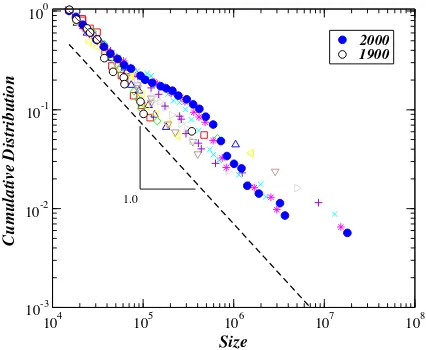
outlier-points. To robust the results obtained by means of the Zipf plots analysis, we also construct the cumulative distribu-tion CDF, that is, the probability of having sizes larger than

a given valueS.Fig. 5shows the CDF for the same data

ana-lyzed inFig. 2. We also ﬁnd that the distributions

approx-imately follow a power law of the formGð>SÞ Sc_{, where}

c

is the Pareto exponent. The maximum-likehood

estima-tion method (MLE)[2]is used to calculate

c

, which leads

to exponents ranging from

c

¼1:32 to

c

¼0:84 for years

1900 and 2000, respectively (seeTable 2). It is noteworthy

that there is a good concordance between the values

esti-mated for

c

and the size-rank exponents

a

, i. e., the

rela-tionship

a

1=

c

is fulﬁlled[44].

Next, we explore the effect of the geographic distribu-tion of cities over the whole statistics described above. To this end, we divide the country into three main regions

namely, north, center and south[46]. In order to get clarity

100 101 102 103

0 1 2 3 4

Local exponent

α

l

1900

10

20

30

40

50

60

70

80

90 2000

(a)

100 101 102 103

rank r

-2

-1 0 1 2

ln

(S/S)*

[image:5.544.124.430.56.300.2]

(b)

Fig. 3.(a) Dependence of local exponentsalon the rank-scale for the Zipf’s plots showed inFig. 2. The variations around the global exponent estimated in Fig. 2, indicate that the global scaling behavior is not true locally. (b) lnðS

=SÞvs. rank-scale for the years showed inFig. 2. In this plot, if the data is close to the zero value, it indicates that the distribution is close to the pure Zipf’s law.

104 105 106 107

Size (t)

104 105 106 107

Size (t+10)

104 105 106 107

1990-2000 1900-1910

1.0

[image:5.544.289.505.357.534.2]

(6)

in the statistics we only considered the data corresponding to the year 2000. The CDF of each region (subset) are

showed inFig. 6, the data indicate that the distributions

for the center and south regions can be well described by

a power law with exponents

c

center¼0:6810:002 and

c

_south¼0:8070:002, whereas the north set leads to

c

north¼0:69220:038, but it is remarkable its deviation from the power law behavior. It is also noteworthy that this deviation observed in the data from the north region,

indicates that the probability of citiesGð>SÞis higher than

the probabilities of the center and the south, for intermedi-ate city sizes. This result conﬁrms the fact that the north region contributes in large extent to the deviation in the

power law behavior of the CSD reported inFig. 2. In order

development between regions, such as the ‘‘bump’’ effect

suggests (seeFigs. 2, 5 and 6). Another peculiarity of

Mex-ican CSD is that for the ten censuses (including the ﬁve

with

a

>1) the size of the largest city (Mexico City) is

greater than the intercept term of the corresponding

ﬁt-tings, unlike those reported by Soo [47], where shows

otherwise for countries with

a

>1.

4. Concluding remarks

The present study shows how along the 20th century

Mexico evolved from low values of

a

at the beginning of

the century up to values above one, since the decade of the 1960’s. These changes coincide with the Mexico’s evo-lution from a rural society towards an urban country. How-ever, nevertheless Mexico passed from an uneven distribution to a more spread population across its terri-tory, the country did not reach the status of developed

country; that is,

a

>1 does not imply economic

develop-ment. Recently, a more suitable interpretation of the

a

behavior was proposed in terms of a concept called

‘‘coher-ence’’[27]. Within this frame the Mexican CSD along the

20th century is better understood. The unequal develop-ment between regions has led to a noticeable deviation from an accurate Zipﬁan behavior even though the mean

a

values are slightly above one. Although some authors

as Soo[47]suggest that political variables appear to matter

more than economic geographic variables in determining the size distribution of cities, the case of Mexico reveals that the economic geography can play a very important role in CSD. In fact, the notorious ‘‘bump’’ observed in

104 105 106 107 108

Size 10-3

10-2

Cumulative Distribution

1.0

Fig. 5.Cumulative distribution of cities for ten censuses. For 1900 data the scaling exponent is close to one (seeTable 2), and for 2000 data the value decreased to 0:79, indicating that the probability of sizesS>105

is bigger than the other datasets from previous years.

104 105 106 107

Size

10-2

10-1 100

Cumulative Distribution

North

Central

South

α=0.7

[image:6.544.41.254.54.229.2]

year 2000

[image:6.544.156.384.465.655.2]

(7)

Mexican data during the last decades of 20th century has a very clear geographic origin. When the Zipf’s plots are observed at local scale, the scaling exponent exhibits vari-ations which indicate that the scaling behavior is not true locally. Thus, only a mean global Zipﬁan analysis is suitable for urban systems of the Mexican-type. In summary, we believe that the CSD in Mexico along the 20th century is a very interesting problem due to peculiarities stemming from its geographic location an its internal social an eco-nomic heterogeneity.

Acknowledgments

We thank I. Fernández-Rosales, R. Hernández-Pérez and I. Reyes-Ramírez for frutiful discussions and suggestions. L. G.-V. and F. A.-B. thank EDI-IPN, COFAA-IPN and CONACYT, México for partial support. E. P. C. thanks to the DGAPA-UNAM [research project [IA300115]: Concen-tration and Diversiﬁcation of the Services Sector in Mexico] for its support.

References

[1]Pareto V. Cours d’economie politique. Librairie Droz; 1964. [2]Newman ME. Contemp Phys 2005;46:323.

[3]Yakovenko VM. In: Ganssmann H, editor. New approaches to monetary theory: interdisciplinary perspectives. Routledge; 2012. p. 104–23.

[4]Hernández-Pérez R, Angulo-Brown F, Tun D. Physica A 2006;359:607.

[5]Kang SH, Jiang Z, Cheong C, Yoon SM. Physica A 2011;390:319. [6]Perc M. J Roy Soc Interface 2012:0491.

[7]Petersen AM, Tenenbaum JN, Havlin S, Stanley HE, Perc M. Sci Rep 2012;2:943.

[8]Oliveira JG, Barabási A-L. Nature 2005;437:1251.

[9]Sornette D. Critical phenomena in natural sciences: chaos, fractals, selforganization and disorder: concepts and tools. Springer Science & Business; 2006.

[10]Perc M. Sci Rep 2013;3:01720.

[11]Kuhn T, Perc Mcv, Helbing D. Phys Rev 2014;X 4:041036. [12]West GB, Brown JH, Enquist BJ. Science 1997;276:122.

[13]Vallina AU. Principles of seismology. Cambridge University Press; 1999.

[14]Gutenberg B, Richter CF. Bull Seismol Soc Amer 1944;34:185.

[15] Bak P, Tang C. J Geophys Res : Solid Earth, 2156-2202 1989;94:15635. Available from: <http://dx.doi.org/10.1029/ JB094iB11p15635>.

[16]Ito K, Matsuzaki M. J Geophys Res: Solid Earth 1990;95:6853. [17]Ioannides YM, Overman HG. Reg Sci Urban Econ 2003;33:127. [18] Marsili M, Zhang YC. arXiv preprint cond-mat/9801289; 1998. [19]Zhang Q, Sornette D. Physica A 2011;390:4124.

[20] Munoz-Diosdado A, Guzmán-Vargas L, Ramírez-Rojas A, del Río-Correa J, Angulo-Brown F. Fractals 2005;13:253.

[21]Pacheco JF, Scholz CH, Sykes LR. Nature 1992;355:71. [22]Dra˘gulescu A, Yakovenko VM. Eur Phys J B 2000;17:723. [23]Dra˘gulescu A, Yakovenko VM. Physica A 2001;299:213.

[24]Dra˘gulescu A, Yakovenko VM. Eur Phys J B-Condens Matter Complex Syst 2001;20:585.

[25]Yakovenko VM, Rosser Jr JB. Rev Mod Phys 2009;81:1703. [26]Banerjee A, Yakovenko VM. New J Phys 2010;12:075032. [27]Cristelli M, Batty M, Pietronero L. Sci Rep 2012;2:1. [28]Eaton J, Eckstein Z. Reg Sci Urban Econ 1997;27:443.

[29]Benguigui L, Blumenfeld-Lieberthal E. Physica A 2009;388:1187. [30] González-Val R. J Reg Sci, 1467-9787 2010;50:952.

[31]Malacarne LC, Mendes R, Lenzi EK. Phys Rev E, 0165-1765 2001;65:017106.

[32]Bee M, Riccaboni M, Schiavo S. Econ Lett, 0165-1765 2013;120:232. [33]Giesen K, Zimmermann A, Suedekum J. J Urban Econ, 0094-1190

2010;68:129.

[34]Black D, Henderson V. J Econ Geog 2003;3:343.

[35]Gisbert FJG, Ivars MM. Revista de Economía Aplicada 2010;18:133. [36]Gangopadhyay K, Basu B. Physica A 2009;388:2682.

[37]Peng G. Physica A 2010;389:3804.

[38]Unikel L. El desarrollo urbano de México. Mexico City: El Colegio de Mexico; 1975.

[39]Moura Jr NJ, Ribeiro MB. Physica A 2006;367:441.

[40] Garza G. La urbanización en México durante el Siglo XX (COLMEX); 2003.

[41] INEGI, Censo general de población y vivienda, 2000; 2002. URL <http://www.inegi.org.mx/est/listacubos/consulta.aspx?p=pob&c= 3>.

[42]Aguilar AG, Graizbord B. In: Geyer HS, editor. International handbook of urban system. Studies of urbanization in advanced and developing countries. Edward Elgar; 2002. p. 419–54. [43]Unikel L. Demografía y Economía 1968;2:139.

[44]Adamic LA, Huberman BA. Glottometrics 2002;3:143. [45]Polèse M, Champagne É. Int Reg Sci Rev 1999;22:102.

Distributions of city sizes in Mexico during the 20th century