From pixels to gestures: learning visual representations for human analysis in color and depth data sequences

From pixels to gestures: learning visual

representations for human analysis in color

and depth data sequences

Antonio Hernández-Vela

Aquesta tesi doctoral

està subjecta a la llicència

Reconeixement- NoComercial

3.0. Espanya

de Creative Commons

.

Esta tesis doctoral está sujeta a la licencia

Reconocimiento -

NoComercial 3.0.

España de

Creative

Commons

.

From pixels to gestures: learning visual

representations for human analysis in color

and depth data sequences

A dissertation submitted by Antonio Hern´andez-Velaat Universitat de Barcelona to fulfil the degree of Doctor en Matem`atiques.

Director Dr. Sergio Escalera

Dept. de Matem`atica Aplicada i An`alisi, Universitat de Barcelona & Centre de Visi´o per Computador

Co-director Prof. Stan Sclaroff

Dept. of Computer Science, Boston University Boston, USA

Thesis Prof. Thomas Baltzer Moeslund

committee Dept. of Architecture, Design and Media Technology, Aalborg University Aalborg, Denmark

Prof. Jordi Vitri`a Marca

Dept. de Matem`atica Aplicada i An`alisi, Universitat de Barcelona & Computer Vision Center

Barcelona, Spain

Dr. Jordi Gonzalez Sabat´e

Dept. Ci`encies de la Computaci´o, Universitat Aut`onoma de Barcelona & Computer Vision Center

Barcelona, Spain

International Dr. Leonid Sigal

evaluators Disney Research &

Dept. of Computer Science, Carnegie Mellon University Pittsbutgh, USA

Dr. Marco Pedersoli

KU Leuven Leuven, Belgium

Prof. Thomas Baltzer Moeslund

Dept. of Architecture, Design and Media Technology, Aalborg University Aalborg, Denmark

This document was typeset by the author using LA_{TEX 2ε.}

The research described in this book was carried out at Universitat de Barcelona and the Computer Vision Center.

Copyright c?2015 by Antonio Hern´andez-Vela. All rights reserved. No part of this publi-cation may be reproduced or transmitted in any form or by any means, electronic or me-chanical, including photocopy, recording, or any information storage and retrieval system, without permission in writing from the author.

ISBN: 978-84-940902-0-2

Acknowledgements

The work presented in this dissertation would not have been possible without the guidance and support of my supervisors. I am extremely thankful to my advisor Sergio Escalera for his continuous efforts, dedication and encouragement during all these years. I am also grateful to Petia Radeva, for her guidance during the early stages of my PhD. Finally, I am especially thankful to my co-advisor Stan Sclaroff for giving me the chance to visit his research group at Boston University and having numerous conversations providing me with valuable feedback and brilliant ideas.

During my short stay in Boston I had the great chance to meet Stan and a lot of nice and brilliant people from the Image and Video Computing research group, from whom I learnt a lot during the five months I spent at Boston University. Among them all, I must give special thanks to Shugao and Kun for his productive conversations and brainstormings. I am also deeply thankful to Ramazan Gokberk and his willingness to help and share useful insights through the numerous e-mail conversations we had during my days in Boston. I would also like to thank Tarique for making my stay in Boston a great time, I felt at home from the very first moment.

I am also really thankful to all my colleagues from the Computer Vision Center, in special to the people I had the great chance to meet during the Master’s academic training: Ekain, Llu´ıs-Pere, David, Jon and Anjan. Special thanks also to Carles, Ivet, Fran, Camp, Joan, Alejandro, Yainubis and all the people I shared a lot of precious moments with; some of you have become really good friends.

I feel very lucky to have seen the birth of the Human Pose and Behavior Analysis (HuPBA) research group at the University of Barcelona. I am really thankful to all my colleagues from HuPBA, in special to Miguel, Miguel ´Angel, V´ıctor, Xavi and Albert. Not only I learnt a lot working with you, but also shared unforgettable moments and laughs.

Muchas gracias a mis amigos de Sabadell, con ellos he pasado gran parte de mi vida y momentos que nunca se olvidan. Gracias tambi´en a las nuevas amistades que he hecho durante estos a˜nos desde que me mud´e a Barcelona; en especial a Rub´en, Oroitz, Xabi, Maria y Aina.

Quiero agradecer a mis padres el apoyo y afecto que siempre me han brindado, as´ı como la educaci´on que me han dado y la paciencia que siempre han tenido conmigo durante todos estos a˜nos. Os quiero mama y papa.

Per ´ultim per`o no per aix`o menys important, vull agra¨ır a la Gisela el seu afecte i la seva paci`encia. Em sento enormement afortunat d’haver-te conegut durant els anys d’aquest viatge. T’estimo molt´ıssim.

Abstract

The visual analysis of humans from images is an important topic of interest due to its relevance to many computer vision applications like pedestrian detection, monitoring and surveillance, human-computer interaction, e-health or content-based image retrieval, among others.

In this dissertation we are interested in learning different visual representations of the human body that are helpful for the visual analysis of humans in images and video sequences. To that end, we analyze both RGB and depth image modalities and address the problem from three different research lines, at different levels of abstraction; from pixels to gestures: human segmentation, human pose estimation and gesture recognition.

First, we show how binary segmentation (object vs. background) of the human body in image sequences is helpful to remove all the background clutter present in the scene. The presented method, based on Graph cuts optimization, enforces spatio-temporal consis-tency of the produced segmentation masks among consecutive frames. Secondly, we present a framework for multi-label segmentation for obtaining much more detailed segmentation masks: instead of just obtaining a binary representation separating the human body from the background, finer segmentation masks can be obtained separating the different body parts.

At a higher level of abstraction, we aim for a simpler yet descriptive representation of the human body. Human pose estimation methods usually rely on skeletal models of the human body, formed by segments (or rectangles) that represent the body limbs, appropriately connected following the kinematic constraints of the human body. In practice, such skeletal models must fulfill some constraints in order to allow for efficient inference, while actually limiting the expressiveness of the model. In order to cope with this, we introduce a top-down approach for predicting the position of the body parts in the model, using a mid-level part representation based on Poselets.

Finally, we propose a framework for gesture recognition based on the bag of visual words framework. We leverage the benefits of RGB and depth image modalities by combining modality-specific visual vocabularies in a late fusion fashion. A new rotation-variant depth descriptor is presented, yielding better results than other state-of-the-art descriptors. More-over, spatio-temporal pyramids are used to encode rough spatial and temporal structure. In addition, we present a probabilistic reformulation of Dynamic Time Warping for gesture seg-mentation in video sequences. A Gaussian-based probabilistic model of a gesture is learnt, implicitly encoding possible deformations in both spatial and time domains.

Resum

La an`alisi visual de persones a partir d’imatges ´es un tema de recerca molt important, degut a la rellev`ancia que t´e a una gran quantitat d’aplicacions dins la visi´o per computador, com per exemple: detecci´o de vianants, monitoritzaci´o i vigil`ancia, interacci´o persona-m`aquina,

e-salut, o sistemes de recuperaci´o d’imatges a partir de contingut, entre d’altres.

En aquesta tesi volem aprendre diferents representacions visuals del cos hum`a, que siguin ´

utils per a la an`alisi visual de persones en imatges i v´ıdeos. Per a tal efecte, analitzem difer-ents modalitats d’imatge com son les imatges de color RGB i les imatges de profunditat, i adrecem el problema a diferents nivells d’abstracci´o, des dels p´ıxels fins als gestos: seg-mentaci´o de persones, estimaci´o de la pose humana i reconeixement de gestos.

Primer, mostrem com la segmentaci´o bin`aria (objecte vs. fons) del cos hum`a en seq¨u`encies d’imatges ajuda a eliminar soroll pertanyent al fons de l’escena en q¨uesti´o. El m`etode presen-tat, basat en optimitzaci´oGraph cuts, imposa consist`encia espai-temporal a les m`ascares de segmentaci´o obtingudes enframesconsecutius. En segon lloc, presentem un marc metodol`ogic per a la segmentaci´o multi-classe, amb la qual podem obtenir una descripci´o m´es detallada del cos hum`a: en comptes d’obtenir una simple representaci´o bin`aria separant el cos hum`a del fons, podem obtenir m`ascares de segmentaci´o m´es detallades, separant i categoritzant les diferents parts del cos.

A un nivell d’abstracci´o m´es alt, tenim com a objectiu obtenir representacions del cos hum`a m´es simples, tot i ´esser suficientment descriptives. Els m`etodes d’estimaci´o de la pose humana sovint es basen en models esqueletals del cos hum`a, formats per segments (o rectangles) que representen les extremitats del cos, connectades unes amb altres seguint les restriccions cinem`atiques del cos hum`a. A la pr`actica, aquests models esqueletals han de complir certes restriccions per tal de poder aplicar m`etodes d’infer`encia que permeten trobar la soluci´o `optima de forma eficient, per`o a la vegada aquestes restriccions suposen una gran limitaci´o en l’expressivitat que aquests models son capa¸cos de capturar. Per tal de fer front a aquest problema, proposem un enfoctop-down per a predir la posici´o de les parts del cos del model esqueletal, introduint una representaci´o de parts de mig nivell basada enPoselets. Finalment, proposem un marc metodol`ogic per al reconeixement de gestos, basat en els

bag of visual words. Aprofitem els avantatges de les imatges RGB i les imatges de profunditat combinant vocabularis visuals espec´ıfics per a cada modalitat, emprantlate fusion. Proposem un nou descriptor per a imatges de profunditat invariant a rotaci´o, que millora l’estat de l’art, i fem servir pir`amides espai-temporals per capturar certa estructura espaial i temporal dels gestos. Addicionalment, presentem una reformulaci´o probabil´ıstica del m`etodeDynamic

Time Warpingper al reconeixement de gestos en seq¨u`encies d’imatges. M´es espec´ıficament,

modelem els gestos amb un model probabilistic Gaussi`a que impl´ıcitament codifica possibles deformacions tant en el domini espaial com en el temporal.

Contents

Acknowledgements i

Abstract iii

Resum v

1 Introduction 1

1.1 Motivation . . . 1

1.2 Objective of this thesis . . . 3

1.3 Contributions . . . 4

1.4 Thesis outline . . . 5

I

Human body segmentation

7

2.2 Basic concepts . . . 11

2.3 Graph topology . . . 12

2.4 Energy minimization in binary problems . . . 12

2.4.1 Unary potential . . . 13

2.4.2 Pair-wise potential . . . 13

2.5 Multi-label generalization . . . 14

2.5.1 α-βswap . . . 14

2.5.2 α-expansion . . . 15

3 Binary human segmentation 19 3.1 Introduction . . . 19

3.2 Related work . . . 19

3.3 GrabCut segmentation . . . 20

3.4 Spatio-temporal GrabCut segmentation . . . 21

3.4.1 Spatial Extension . . . 22

3.4.2 Temporal extension . . . 22

3.5 Experiments . . . 23

3.5.1 Data . . . 23

3.5.2 Methods . . . 24

3.5.3 Validation measurements . . . 25

3.5.4 Spatio-Tempral GrabCut Segmentation . . . 26

viii CONTENTS

3.5.5 Face alignment . . . 26

3.5.6 Human pose estimation . . . 30

3.6 Discussion . . . 34

4 Multi-label human segmentation 35 4.1 Introduction . . . 35

4.2 Related work . . . 35

4.3 Method overview . . . 36

4.4 Random Forests for body part recognition . . . 37

4.5 Multi-limb human segmentation . . . 40

4.6 Experiments . . . 41

4.6.1 Data . . . 42

4.6.2 Methods and validation . . . 43

4.6.3 Random forest pixel-wise classification results . . . 43

4.6.4 Multi-label segmentation results . . . 44

4.7 Discussion . . . 47

II

Human Pose Estimation

51

5.2 Pictorial structures . . . 56

5.2.1 Inference . . . 57

5.2.2 Learning . . . 57

5.3 Deformable Part Models . . . 58

5.3.1 Inference . . . 59

5.3.2 Learning . . . 59

6 Contextual Rescoring for Human Pose Estimation 61 6.1 Introduction . . . 61

6.2 Related work . . . 61

6.3 Method overview . . . 63

6.4 Mid-level part representation . . . 64

6.4.1 Hierarchical decomposition . . . 64

6.4.2 Poselet discovery . . . 65

6.5 Contextual rescoring . . . 66

6.6 Deformable part model formulation . . . 68

6.7 Pictorial structure formulation . . . 69

6.8 Experiments . . . 71

6.8.1 Data . . . 71

6.8.2 Methods and validation . . . 72

6.8.3 Experiments with deformable part models . . . 73

6.8.4 Experiments with pictorial structures . . . 75

CONTENTS ix

III

Gesture Recognition

85

7 BoVDW for gesture recognition 89

7.1 Introduction . . . 89

7.2 Related work . . . 90

7.3 Bag of Visual Words . . . 91

7.4 Bag of Visual and Depth Words . . . 92

7.4.1 Keypoint detection . . . 92

7.4.2 Keypoint description . . . 92

7.4.3 BoVDW histogram . . . 94

7.4.4 BoVDW-based classification . . . 94

7.5 Experiments . . . 95

7.5.1 Data . . . 95

7.5.2 Methods and validation . . . 95

7.5.3 Results . . . 96

7.6 Discussion . . . 96

8 PDTW for continuous gesture recognition 99 8.1 Introduction . . . 99

8.2 Related work . . . 99

8.3 Dynamic Time Warping . . . 100

8.4 Handling variance with Probability-based DTW . . . 101

8.4.1 Distance measures . . . 103

8.5 Experiments . . . 103

8.5.1 Data . . . 103

8.5.2 Methods and validation . . . 104

8.5.3 Results . . . 105

8.6 Discussion . . . 105

IV

Epilogue

109

9.2 Final conclusions . . . 112

9.3 Future work . . . 114

A Code and Data 117

B Publications 119

List of Figures

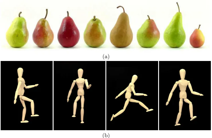
1.1 (a) Pears are an example of objects which are simple to detect, since little variations can be found among different samples. (b) In contrast, articulated objects can suffer significant changes in their shape given their high deforma-bility, hence are harder to detect. . . 2 1.2 Understanding still life scenes (a) just requires to detect the objects it is

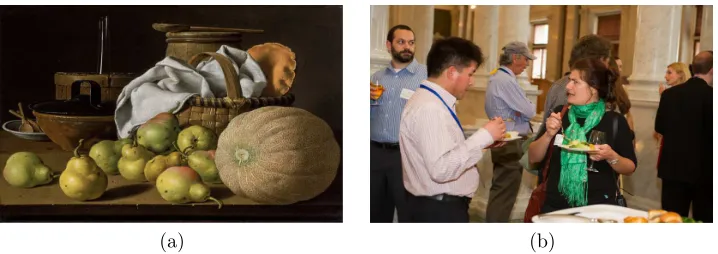
composed of. In contrast, understanding scenes of people (b) entail human pose detection, facial expression recognition, or gesture recognition (in the case of video sequences). . . 3 1.3 (a) Binary human body segmentation. (b) Multi-label human body

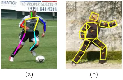
segmen-tation. . . 4 1.4 Skeleton-based representations of the human body formed by (a) segments,

and (b) rectangles. . . 4 1.5 Gestures for letters “J” and “Z” in the American Sign Language. . . 5

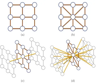
2.1 (a) Example topology ofG for a typical computer vision application for 2-D images. (b) Example of a cut and the resulting labeling of the nodes. . . 12 2.2 Common graph topologies in computer vision applications. 2-D grids

(im-ages): (a) 4-connectivity, and (b) 8-connectivity. 3-D grids (video sequences): (c) 6-connectivity, and (d) 26-connectivity (brown edges show intra-frame con-nections, yellow edges show inter-frame connections). . . 13 2.3 Graph topologyGαforα-expansion energy minimization. Additional aribtrary

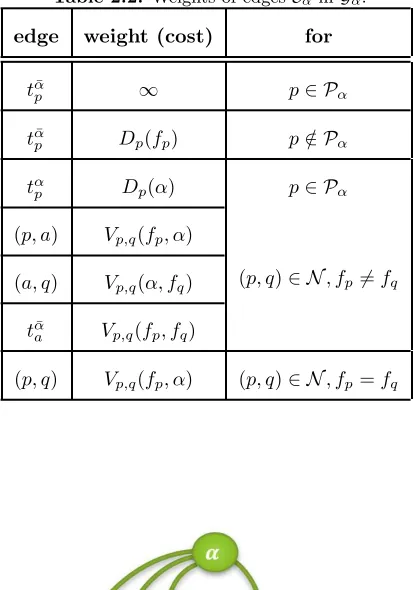
nodesap,q and respectivet−links tαp¯ are depicted in red color. . . 17 3.1 STGrabcut pipeline example: (a) Original frame, (b) Seed initialization, (c)

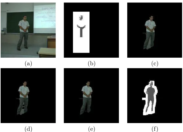
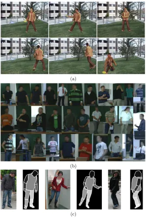
GrabCut, (d) Probabilistic re-assignment, (e) Refinement and (f) Initialization mask forIt+1_{.. . . . 23} 3.2 (a) Samples of the cVSG corpus and (b) UBDataset image sequences, and (c)

HumanLimb dataset. . . 25 3.3 From left to right: left, middle-left, frontal, middle-right and right mesh fitting. 28 3.4 Segmentation examples of (a) UBDataset sequence 1, (b) UBDataset sequence

2 and (c) cVSG sequence. . . 29 3.5 Samples of the segmented cVSG corpus image sequences fitting the different

AAM meshes. . . 29 3.6 Pose recovery results in cVSG sequence. . . 31 3.7 Application of the whole framework (pose and face recovery) on an image

sequence. . . 31

xii LIST OF FIGURES

3.8 Human Limb dataset results. Upper row: body pose estimation without ST-GrabCut segmentation. Lower row: body pose estimation with ST-ST-GrabCut segmentation. . . 33 3.9 Application of face alignment on human body limb dataset. . . 33

4.1 Pipeline of the presented method, including the input depth information, Ran-dom Forest, Graph-cuts, and the final segmentation result. . . 38 4.2 Graph topology introducing temporal coherence. . . 41 4.3 Interface for semi-automatic ground-truth generation. . . 42 4.4 Qualitative results; Ground Truth (a), RF inferred results (b), RWalks results

(c), frame-by-frame GC results (d), and Temporally-coherent GC results (e). 46 4.5 Results from RF classification in the case of hands. First row shows the

ground-truth for two examples. Second row shows the RF classification re-sults. Third row shows the finalα-expansion GC segmentation results. . . 48 4.6 Comparison of results without (a) and with (b) spatially-consistent labels. . . 48

5.1 Pedestrian detection as a classic sliding-window approach for object detection. HOG features extracted from candidate bounding boxes in the image are tested against a Linear SVM trained on images of people, which predicts a positive (green) or negative (red) answer for each candidate window. . . 55 5.2 (a) Sample pictorial structure for human pose estimation; blue rectangles

de-pict the different parts of the model (corresponding to parts of the human body) and yellow springs show the flexible connections between parts. (b) The corresponding CRF for the pictorial structure model in (a); blue nodes represent the parts of the model and yellow edges codify the spring-like con-nections. . . 56 5.3 Different poses of the human body. . . 58

6.1 Proposed pipeline for human pose estimation. Given an input image, a set of basic and mid-level part detections is obtained. For each basic part detection

li, a contextual representation is computed based on relations with respect to the set of mid-level part detections. Using these contextual representations, basic part detections are rescored using a classifier for that particular basic part class. The original and rescored detections for all basic parts are then used in inference on a pictorial structure (PS) model to obtain the final pose estimate. . . 63 6.2 Sample Poselet templates. Body joints are shown with colored dots, and their

corresponding estimated Gaussian distributions as blue ellipses. . . 64 6.3 Two sample images depicting a reference detection bounding boxBiin yellow

(for the right ankle), and the set of contextual mid-level detectionsPin blue, orange and green for the upper body, lower body and full body, respectively. 67 6.4 Sample poselets from the LSP dataset. (a) Poselets with highest precision.

(b) Poselets discovered by our selection method, maximizing precision and enforcing covering of the validation set. . . 73 6.5 Qualitative results for the proposed rescoring approach incorporated in the

DPM model from Yang and Ramanan [96], in the LSP dataset . . . 74 6.6 Qualitative results for the proposed rescoring approach incorporated in the

LIST OF FIGURES xiii

6.7 Position prediction comparison in (a) LSP and (b) PARSE datasets. In each plot, PCP performance is shown as a function ofβu

p. We compare our proposed rescoring approach when usingP= 47 poselets, automatically selected by our proposed poselet discovery method, w.r.t. the position prediction from [69] withP = 1,013 andP = 47 poselets. . . 76

6.8 Comparison of different mid-level representations in (a) LSP and (b) PARSE datasets. In each plot, PCP performance is shown as a function ofβu

p. We compare our poselet selection maximizing precision and enforcing covering against (1) the manual hierarchical decomposition from [69], (2) selecting the poselets with maximum precision, and (3) the poselet selection greedy method from [15]. . . 77

6.9 Failure cases in (a) LSP and (b) PARSE datasets. Our proposed method cannot recover the human pose correctly, mainly due to upside-down poses and cases with extra people close to the actual subject. . . 80

6.10 Contextual feature selection histograms computed from the learnt decision treesqθ, grouped by subsets of joints: (a) upper-body limbs, (b) lower-body limbs, (c) head & torso, and (d) full body. . . 81

6.11 Qualitative results on LSP dataset. (a) Gaussian-shaped position prediction from [69], (b) Estimated pose from [69] (just predicting position), (c) Esti-mated pose from [69] (full model), (d) Position prediction with our proposed rescoring, and (e) Our results. White crosses in columns (a) and (d) show the part being rescored in each case; from the first row to the last one: rightmost ankle, rightmost wrist, leftmost ankle, leftmost wrist. . . 82

6.12 Qualitative results on PARSE dataset. (a) Gaussian-shaped position predic-tion from [69], (b) Estimated pose from [69] (just predicting posipredic-tion), (c) Estimated pose from [69] (full model), (d) Position prediction with our pro-posed rescoring, and (e) Our results. White crosses in columns (a) and (d) show the part being rescored in each case; from the first row to the last one: right ankle, right wrist, right ankle, left ankle. . . 83

7.1 (a) An example of the bag of words representation for text classification. (b) Bag of visual words representation for image categorization. . . 92

7.2 BoVDW approach in a Human Gesture Recognition scenario. Interest points in RGB and depth images are depicted as circles. Circles indicate the assign-ment to a visual word in the shown histogram – computed over one spatio-temporal bin. Limits of the bins from the spatio-spatio-temporal pyramids decom-position are represented by dashed lines in blue and green, respectively. A detailed view of the normals of the depth image is shown in the upper-left corner. . . 93

7.3 (a) Point cloud of a face and the projection of its normal vectors onto the planePxy, orthogonal to the viewing axisz. (b) VFHCRH descriptor: Con-catenation of VFH and CRH histograms resulting in 400 total bins . . . 94

7.4 Confusion matrices for gesture recognition in each one of the 20 development batches. . . 97

xiv LIST OF FIGURES

8.2 (a) Different sequences of a certain gesture category and the median length sequence. (b) Alignment of all sequences with the median length sequence by means of Euclidean DTW. (c) Warped sequences set ˜Sfrom which each set of

t-th elements among all sequences are modelled. (d) Gaussian Mixture Model learning with 3 components. . . 102 8.3 Examples of idle gesture detection on the Chalearn data set using the

probability-based DTW approach. The line below each pair of depth and RGB images represents the detection of a idle gesture (step up: beginning of idle gesture, step down: end) . . . 106

List of Tables

1.1 Symbols and conventions for chapters 2- 4 . . . 9

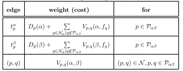
2.1 Weights of edgesEαβ in Gαβ. . . 15

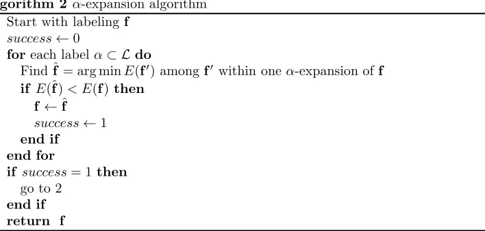
2.2 Weights of edgesEα inGα. . . 17

3.1 GrabCut and ST-GrabCut Segmentation results on cVSG corpus. . . 26

3.2 AAM mesh fitting on original images and segmented images of the cVSG corpus. 30 3.3 Face pose percentages on the cVSG corpus. . . 30

3.4 Pose estimation results: overlapping of body limbs based on ground truth masks. . . 31

3.5 Overlapping percentages between body parts (intersection over union), wins (comparing the highest overlapping with and without segmentation), and matching (considering only overlapping greater than 0.6). ∗_{STGrabCut was} used without taking into account temporal information. . . 32

4.1 Average per class accuracy in % calculated over the test samples in a 5-fold cross validation. ψθ represents features of the depth comparison type from Eq. (4.1), while ˆψθ - the gradient comparison feature from Eq. (4.13). Omax is the upper limit of theuand voffsets, and dmax stands for the maximal depth level of the decision trees. . . 44

4.2 Average per class accuracy in % obtained when applying the different GC approaches –TC: Temporally coherent, Fbf: Frame-by-Frame– , and the best results from the RF probabilities [79] and the RWalks segmentation algorithm [44], in the first and second rows, respectively. . . 45

4.3 Symbols and conventions for chapters 5- 6 . . . 53

6.1 List of contextual features included incBi,Bp. For clarification, the detection score is encoded classwise in a sparse vector, i.e. a vector of size P set to zeros except the position corresponding to the class of the detection, which contains the detection score. . . 68

6.2 Pose estimation results for LSP dataset. The table shows the PCP for each part separately, as well as the mean PCP. Columns with two values indicate the PCP for the left and right parts, respectively. The methods in the table are grouped according to the features they use, namely: HOG (H), HOG + RGB (HC) and Shape context (SC). We compare our rescoring proposal and mid-level image representation computed with our proposed poselet selection method, against the state of the art. ∗ They use extra 11,000 images for training. ⋄14 parts. †(P = 1,013). ‡(P= 47, pred-pos only). . . 78

xvi LIST OF TABLES

6.3 Pose estimation results for PARSE dataset. See Table 6.2 for table legend. *They use extra 11,000 images for training. ⋄14 parts. † (P = 1,013). ‡

(P = 47, pred-pos only). . . 79 6.4 Running time (in seconds) of the test pipelines from [69] (Algorithm 8) and

our proposal (Algorithm 9). . . 81 6.5 Symbols and conventions for chapters 7- 8 . . . 87

7.1 Mean Levenshtein distance for RGB and depth descriptors. . . 96 7.2 Mean Levenshtein Distance of the best RGB and depth descriptors separately,

as well as the 2-fold and 3-fold late fusion of them. Results obtained by the baseline from the ChaLearn challenge are also shown. Rows 1 to 20 represent the different batches.

. . . 98

Chapter 1

Introduction

1.1

Motivation

In the quest for artificial intelligence, the ultimate goal could be envisioned as the creation of “intelligent” robots, i.e. robots which have an “intelligent” behavior, following the guidelines of our human intelligence. This intelligence can be defined in many different ways, depending on the different processes that take place in our brains in order to perform a certain task. Among them all, it has been proven that visual intelligence –the reasoning processes related to our visual system– plays an important role in our global intelligent behavior, and this fact can be easily illustrated by imagining ourselves performing daily tasks like commuting or even preparing breakfast without perceiving and processing visual information.

Visual intelligence can be defined as understanding the 3-D spatial world that surrounds us from 2-D projections of it,i.e. images, captured by our retinae. While we are not aware of it, our brain is constantly processing visual information in order to understand our environ-ment, and it is pretty good at it, though it is a really challenging task. In our daily lives we are generally able to recognize objects, people and faces without much trouble, even though our 3-D world is full of objects that occlude each other and we are able to infer it from just 2-D projections. Moreover, we are able to recognize objects under different viewpoints or projections, usually implying a change in their appearance. However, when trying to accomplish these tasks artificially by means of computers, we realize the challenging nature of the problem and the power of our brains.

Computer vision is the field of Artificial Intelligence dedicated to the acquisition and processing of images, trying to replicate the human visual intelligence using computer soft-ware and hardsoft-ware. Visual tasks like object recognition have been vastly researched during many years and they are still a challenge for researchers in the field. The main problems to face when designing algorithms for object recognition are: changes in illumination, changes in viewpoint, presence of occlusions or object class variability, among others. While some objects may have little appearance variations in size, color or shape things get complicated in the case of articulated objects composed by movable parts (see Fig. 1.1). Such deformable objects can eventually change their shape appearance considerably, thus complicating the process of learning patterns of their appearance.

Besides object detection and recognition, people detection has caught the attention of many researchers, because of its multiple applications,e.g. pedestrian detection, monitoring and surveillance, human-computer interaction e-health, or content-based image retrieval. Detecting people in images is challenging, in the first place, due to the the articulated

2 INTRODUCTION

(a)

(b)

Figure 1.1: (a) Pears are an example of objects which are simple to detect, since

little variations can be found among different samples. (b) In contrast, articulated objects can suffer significant changes in their shape given their high deformability, hence are harder to detect.

nature of the human body: people can adopt a wide range of poses and consequently, the body shape has a large variability. Not only that, but certain poses may also incur in self-occlusions of some body parts, thus making it more difficult to detect. In addition, different clothing can also result in slight changes in the shape of the body, plus a significant change in color appearance. Finally, humans are animated entities that are able to perform different actions with different purposes in comparison with static objects. Therefore, understanding images of people is much more complicated, since human behavior or social signal come into play (see Fig. 1.2).

1.2. Objective of this thesis 3

(a) (b)

Figure 1.2: Understanding still life scenes (a) just requires to detect the objects it

is composed of. In contrast, understanding scenes of people (b) entail human pose detection, facial expression recognition, or gesture recognition (in the case of video sequences).

pose estimation and gesture recognition for human-computer interaction. Nevertheless, such low-cost range imaging solutions still present some issues in outdoor applications, rendering them almost useless in those cases, in front of RGB cameras.

1.2

Objective of this thesis

In this thesis, we are interested in learning different visual representations of the human body that are helpful for the visual analysis of humans in images and video sequences. To that end, we analyze both RGB and depth image modalities and address the problem from three different research lines, at different levels of abstraction; from pixels to gestures:

1. Human body segmentation:At the lowest level of abstraction, we consider

segmen-tation in order to obtain a pixel-wise represensegmen-tation of the human body. Segmensegmen-tation methods aim to partition an image in different segments, usually containing different objects or classes of interest. On one hand, we consider binary segmentation (object vs. background) as a pre-processing step in order to remove all the background clutter. After that, further techniques for a deeper analysis of the human body (e.g. human pose estimation) can be applied in much smaller image regions of interest, where the actual body is located. On the other hand, multi-label segmentation methods can be also applied for a much more detailed pixel categorization; instead of just obtian-ing a binary representation separatobtian-ing the human body from the background, finer segmentation masks can be obtained separating the different body parts (see Fig 1.3).

2. Human pose estimation: At a higher level of abstraction, we aim for a simpler

4 INTRODUCTION

(a) (b)

Figure 1.3: (a) Binary human body segmentation. (b) Multi-label human body

segmentation.

(a) (b)

Figure 1.4: Skeleton-based representations of the human body formed by (a)

seg-ments, and (b) rectangles.

3. Gesture recognition: A deeper analysis and understanding of human behavior from

visual information, usually requires to take into account the temporal dimension,i.e. to process video sequences instead of just still images. Topics like gesture recognition aim to detect specific motion patterns outlined by different body parts along time. Usually, these motion patterns have to be put in correspondence with finer-grained spatial configurations of the body parts,e.g. the hands, in order to detect complex gestures like in sign language (see Fig. 1.5), for example. Furthermore, gesture recognition can be used for recognizing higher-level semantic units related to human behavior, e.g. human activity recognition.

1.3

Contributions

We summarize the contributions of this thesis in the following list, classified by the corre-sponding research line:

1.4. Thesis outline 5

Figure 1.5: Gestures for letters “J” and “Z” in the American Sign Language.

• We propose a fully-automatic method for binary segmentation of people (i.e. segment-ing the human body from the background) appearsegment-ing in video sequences. Our pro-posed method extends the formulation of GrabCut to video sequences, incorporating spatio-temporal consistency by means of Mean Shift clustering (spatial consistency) and a mask initialization algorithm that enforces smooth changes between consecutive frames (temporal consistency).

• We present a generic framework for spatio-temporally consistent multi-label object segmentation based on Random Forest classification and Graph-cuts theory. The presented methodology is applied to human limb segmentation in depth data, yield-ing a more detailed segmentation of the human body compared to a simple fore-ground/background mask.

Human pose estimation

• We propose a contextual rescoring methodology for predicting the position of body parts in a human pose estimation framework based on pictorial structures. This rescor-ing approach encodes high-order body part dependencies by means of a mid-level part representation, yielding more confident position predictions of the body parts while keeping a tree-structured CRF topology in the pictorial structure framework.

• We propose an algorithm for the fully-automatic discovery of a compact contextual mid-level part representation based on Poselets. This contextual representation is able to capture pose-related information that is exploited by our proposed contextual rescoring methodology for human pose estimation.

Gesture recognition

• We propose a framework for gesture recognition based on the bag of visual words framework. We leverage the benefits of RGB and depth image modalities by combining modality-specific visual vocabularies in a late fusion fashion. A new rotation-variant depth descriptor is presented, yielding better results than other state-of-the-art de-scriptors. Moreover, spatio-temporal pyramids are used to encode rough spatial and temporal structure.

• We present a probabilistic reformulation of Dynamic Time Warping for gesture seg-mentation in video sequences. A Gaussian-based probabilistic model of an idle gesture is learnt, implicitly encoding possible deformations in both spatial and time domains.

1.4

Thesis outline

6 INTRODUCTION

recognition. For the reader’s convenience, the symbol notation of each part is summarized in a table at the beginning of each part. Given the multidisciplinary nature of this thesis, most of the chapters are structured in a similar way, including an introduction, then present-ing related work, method formulation, experimental section and a final discussion section summarizing the contributions.

In Part I, we start in chapter 2 by introducing the basis of Graph cuts optimization for both the binary case and its multi-label generalization, used in the following chapters. In chapter 3 we present a method for binary segmentation of subjects in video sequences using graph cuts theory. Finally, in chapter 4 we take advantage of the multi-label generalization of the graph cuts framework to present a methodology for multi-limb segmentation of upper bodies in multi-modal video sequences including RGB and depth data.

Part II is dedicated to Human Pose Estimation. Chapter 5 introduces two widely used frameworks for articulated object detection and consequently, for the problem of human pose estimation: deformable part models and pictorial structures. In chapter 6 we present a contextual rescoring method for obtaining more robust part detections in part-based object detection frameworks like those introduced in chapter 5.

Part III contains our contributions in Gesture Recognition. In chapter 7 we present a Bag-of-Visual-and-Depth-Words representation for gesture recognition in multi-modal RGBD data sequences. In Chapter 8 we propose an extension of Dynamic Time Warping by defining a distance metric based on a probabilistic formulation.

Finally, conclusions and contributions of the thesis are summarized in chapter 9, as well as future lines of research.

Part I

Human body segmentation

Symbol notation in Part I

Table 1.1: Symbols and conventions for chapters 2- 4

G=<V,E> Graph formed by a set of nodesV and a set of edgesE P Set of non-terminal nodes

{s, t} Set of terminal nodes: sourcesand sinkt

N Set of non-terminal edges

T ={ts

p, ttp|p∈ P} Set of terminal links

C={Ps,Pt} A cut onG: a binary partition of nodesP intoPs,Pt

L Set of labels

f={fp|p∈ P} Labeling of non-terminal nodesP E Energy function

D Unary potential inE V Pair-wise potential inE α, β, γ Random labels

I Image

z Array of pixels inI

zi= (xi, yi, Ri, Gi, Bi) Pixel information: spatial coordinates (xi, yi) and color compo-nentsRi, Gi, Bi

N Number of pixels inI T ={TF, TB, TU} GrabCut trimap

θ={π, µ, σ} GMM parameters: mixing weights, mean and covariance matrix

k Array of pixel GMM component assignments

β Statistics of boundaries inI

Γ Pair-wise potential weight.

I={It

|t= 1, ..., M} Video sequence

M Number of frames in the video sequenceI

B Bounding box around the detected person

R Central subregion ofB hskin Skin color model

δ(zi, hskin) Function that returns a subset of pixels with high likelihood P(hskin|zi)

mh Mean-shift modes F Image segmentation mask

STe Structuring element O Overlapping factor

g Texture vector

µg, σs2 Mean and variance of elements ofg

10

¯

x Mean shape

¯

g Mean texture

Qs,Qg Matrices designing modes of variation

X A shape in the image

St(x) Similarity transformation

E Fitting error

ℑF,ℑR,ℑL Face meshes for frontal, right lateral and left lateral views L={li|i= 1, ..., P} Configuration of body partsli

li= (x, y, o) Parametrization of partli: postion (x, y) and orientationo Υ Unary potential in energy function for human pose estimation Ψ Pair-wise potential in energy function for human pose estimation

λ∈Λ Random tree in random forest Λ

ψθ(zi) Depth comparison feature for pixelzi θ= (u, v) A pair of offsets

Φ Set of node splitting criteria φ= (θ, τ)

τ Threshold onψθ

Z Set of random training pixels to trainλ

ZL, ZR Subsets of pixels resulting from a splitting node inλ G(·) Information gain function

H(·) Entropy function

Pλ(c|zi) Probability density function stored at the leafs ofλ,c∈ L dmax Averaged maximum depth level of trees in Λ

Omax Upper limit for the module of offsetθ Ω1(fi, fj),Ω2(fi, fj) Label cost functions between labelsfi, fj

rs

c Friedman relative ranking for strategysand labelc∈ L Rs Friedman mean ranking for strategys

k Number of strategies for Friedman test

Chapter 2

Graph cuts optimization

2.1

Introduction

Graph cuts optimization has been extensively used in different Computer Vision applications like image segmentation, image restoration, stereo matching, or any other problem that can be formulated as an energy minimization problem [17, 20]. Graph cuts are able to find the optimal solution (the one with minimum energy) in the case of binary problems, and near-optimal approximate solutions in the multi-label case, as long as the defined energy function satisfies some conditions.

In this chapter we review the theory behind Graph cuts optimization and its properties, which will be later applied in chapters 3- 4 for segmenting the human body.

2.2

Basic concepts

LetG=<V,E>be a graph formed by a set of nodesVand a set of edgesEconnecting them. The set of nodesV ={s, t} ∪ P can be decomposed in two subsets. On one hand, we note the terminal nodess (source) andt(sink) (light-blue-filled nodes in Fig. 2.1(a)). On the other, we denote byP the set of non-terminal nodes (dark-blue-lined nodes in Fig. 2.1(a)). The edgesE=N ∪T can be also divided in two classes. We first denote byN ={(p, q)∈ E |p, q∈ P}the set of edges connecting two non-terminal nodes, also referred to asn−links

(see brown-colored edges in Fig. 2.1(a)). Secondly, we consider the set oft−links,i.e. the links connecting a non-terminal node with the terminal nodessandt: T ={ts

p, ttp|p∈ P}, wheretsp= (s, p), t

t

p= (p, t) (black-colored edges in Fig 2.1(a)). Finally, every other edge in the graph is assigned a cost, defined by the energy function that we want to minimize.

A “cut”C ={Ps,Pt}of the graphG is a partitioning of the nodesP into two disjoint subsets Ps and Pt, named after the terminal nodes s (source) and t (sink), respectively. Therefore, a cut unequivocally assigns each nodep∈ P to one of thet−links, producing a labellingf ={fp|p∈ P}, wherefp∈ L (L={0,1}for the binary case). The cost of a cutC is then defined as the sum of the costs of edgesE in the graphG. An example of a cut is shown as an orange dotted line in Fig. 2.1(b), and the corresponding partitioning of the nodes in green and purple colors.

12 GRAPH CUTS OPTIMIZATION

(a) (b)

Figure 2.1: (a) Example topology ofGfor a typical computer vision application for

2-D images. (b) Example of a cut and the resulting labeling of the nodes.

2.3

Graph topology

In computer vision applications, typical topologies forGare in the shape ofN-D grids, being

N= 2 the most common case, arranging the nodes in the graph following the 2-D lattice of an image (see Fig. 2.1). Given two contiguous pixelsiandjin an imageI, nodesp, q ∈ P

represent them in the graph, and an edge (p, q)∈ N represents their neighborhood property. Similarly, we can imagine a 3-D grid topology in order to process spatio-temporal volumes

i.e. video sequences.

Different neighboring patterns can be considering to give shape to theN-D grid topolo-gies. The most popular neighborhood patterns in the case of 2-D lattices, are the 4-connectivity and the 8-4-connectivity. While the former just considers two nodes to be con-tiguous if they share either the x or they coordinates (see Fig. 2.1(a-b)), the latter also considers nodes placed in the diagonals. Similarly, typical neighborhood systems in a 3-D grid are 6-connectivity or 26-connectivity (see Fig. 2.1(c-d)).

2.4

Energy minimization in binary problems

Themin−cut/max−f low algorithm is able to efficiently find the exact solutionf with minimum energy, as long as the problem is binary (L ={0,1}), and the potentials in the defined energy function are of order 2 at most. In other words, only functions which can be expressed as a sum of functions that take into account at most 2 variables at a time, are allowed. The standard form of such energy functionsE is:

E(f) =? p∈P

Dp(fp) + ?

(p,q)∈N

Vp,q(fp, fq), (2.1)

2.4. Energy minimization in binary problems 13

(a) (b)

(c) (d)

Figure 2.2: Common graph topologies in computer vision applications. 2-D grids

(images): (a) 4-connectivity, and (b) 8-connectivity. 3-D grids (video sequences): (c) 6-connectivity, and (d) 26-connectivity (brown edges show intra-frame connections, yellow edges show inter-frame connections).

2.4.1

Unary potential

The unary potentialDp in Eq. 2.1, computes the cost of assigning the labelfp to node p, based on observed data. This cost is assigned to edgestspandt

t

pin casefp= 1 andfp= 0, respectively.

A common definition of the unary potential in many computer vision applications is the negative log likelihood:

Dp(fp) =−logP(p|fp). (2.2) This way, the likelihood probabilityP(p|fp) (which we are interested in maximizing in our solution) is converted to a cost, so finding the minimum value (remember we are interested in minimizingE) corresponds to finding the maximum likelihood.

2.4.2

Pair-wise potential

The pair-wise potential (Vp,qin Eq. 2.1) is the responsible for assigning costs to edges (p, q)∈

14 GRAPH CUTS OPTIMIZATION

labels fp, fq to contiguous nodesp, q, based on observed data like in the case of the unary potential. This pair-wise potential is meant to enforce “smoothness” in the solution, fostering similar pixels to have the same label. Therefore,Vp,q is meant to be a non-convex function of|fp−fq|,i.e. a discontinuity-preserving function.

An important and widely used example for such discontinuity-preserving function is the Potts model:

Vp,q(fp, fq) = [fp?=fq], (2.3) where [χ] is an indicator function that takes the value 1 if condition χ is satisfied, or 0 otherwise. Therefore, this model encourages solutions consisting on different regions such that pixels in the same region are assigned the same label.

2.5

Multi-label generalization

Although graph cuts optimization is inherently binary, the same framework has been also extended to multi-label problems 1_{,i.e. when |L| >2. The generalization of a binary cut}

C={S,T }to a multi-label case can be then formulated as a partitioningP={Pl|l∈ L}, wherePl={p∈ P |fp=l}.

Given that|L|>2, the number of label combinations in the boundaries of a possible cut

C can be much higher (it grows quadratically on |L|). Hence, more interesting versions of the Potts model can be taken into consideration where different values can be assigned to different pairs of labelsα, β∈ L.

Exact multi-label optimization is only possible when labelsLcan be linearly ordered, and the pair-wise potential is defined as a specific convex functionVp,q=|fp−fq|, but in practice for computer vision applications, the obtained result is oversmoothed. However, there are more interesting algorithms that get approximate solutions: α-βswap andα-expansion. We review them in the following subsections.

2.5.1

α

-

β

swap

This algorithm is able to find an approximate solution (without any guarantee of closeness to the optimal solution), as long as the pair-wise potential satisfies the following conditions for any pair of labelsα, β∈ L:

V(β, α) =V(α, β)≥0 (2.4)

V(α, β) = 0 ⇐⇒ α=β. (2.5)

In case the above mentioned conditions are satisfied, we callV a semi-metric on the space of labelsL.

The α-β swap algorithm (see Algorithm 1) is based on the concept of a “swap” move, as its name indicates. A “swap” move between labelsα, β∈ Lis summarized as generating a new labelingf′ (partitioningP′) from an arbitrary labelingf, such thatPl=Pl′ for any labell?=α, β. In other words, an α-βswap move from f to f′ can just swap labels fromα

toβ, or viceversa.

We denote by Gαβ =<Vαβ,Eαβ >the graph construction for multi-label optimization withα-β swap, which is very similar to that presented for the binary case,G. In this case, the set of nodesVαβ={α, β} ∪ Pαβ is formed by terminal nodesαandβ, plus non-terminal

1_{While we use here the term “multi-label” following the bibliography, we think it would be more}

2.5. Multi-label generalization 15

Algorithm 1α-β swap algorithm

1: Start with labeling f

2: success←0

3: foreach pair of labels {α, β} ⊂ Ldo

4: Find ˆf = arg minE(f′) amongf′ within oneα-β swap off

5: if E(ˆf)< E(f)then

6: f ←ˆf

7: success←1

8: end if

9: end for

10: if success= 1then 11: go to 2

12: end if

13: return f

Table 2.1: Weights of edgesEαβ inGαβ.

edge weight (cost) for

tα

p Dp(α) + ? q∈Np|q /∈Pαβ

Vp,q(α, fq) p∈ Pαβ

tβ

p Dp(β) + ? q∈Np|q /∈Pαβ

Vp,q(β, fq) p∈ Pαβ

(p, q) Vp,q(α, β) (p, q)∈ N, p, q∈ Pαβ

nodesPαβ=Pα∪ Pβ. Similarly, the set of edgesEαβ=N ∪ Tαβ, whereN is the set of edges connecting non-terminal nodes, and Tαβ ={tαp, tβp |p∈ Pαβ}. The assignment of costs to edgesEαβ is summarized in Table 2.1.

Finally, energy minimization is performed by a min−cut algorithm on Gαβ, like in the binary case. It has been proven by Boykov et al. [19] that finding the solution ˆf with minimum energy (step 4 in Algorithm 1) is equivalent to finding the minimum cutConGαβ.

2.5.2

α

-expansion

In contrast to the previous algorithm,α-expansion ensures finding a solution within a known factor (as small as 2) from the optimal one. However, in addition to conditions in Eq. 2.4 and Eq. 2.5, the following condition must be also satisfied:

V(α, β)≤V(α, γ) +V(γ, β), (2.6) for anyα, β, γ ∈ L. If all these conditions are satisfied, then we say that V is a metric on the space of labelsL, andα-expansion can be successfully applied.

16 GRAPH CUTS OPTIMIZATION

Algorithm 2α-expansion algorithm

1: Start with labeling f

2: success←0

3: foreach labelα⊂ Ldo

4: Find ˆf = arg minE(f′_{) amongf}′ _{within oneα-expansion off}

5: if E(ˆf)< E(f)then

6: f ←ˆf

7: success←1

8: end if

9: end for

10: if success= 1then

11: go to 2

12: end if

13: return f

The graph construction for α-expansion is quite different from the previous case. In this case, a graph Gα =< Vα,Eα > is built, where the set of nodes Vα contains not only the terminal nodes αand ¯α and non-terminal nodesP, but an additional set of arbitrary non-terminal nodesap,q:

Vα={α,α¯} ∪ P ∪ ?

(p,q)∈N,fp?=fq

ap,q. (2.7)

Arbitrary nodesap,qare introduced in the graph connecting neighboring nodesp, q∈ N that have different assigned labels,i.e.fp?=fq(see Fig. 2.3). The set of edges is then defined as:

Eα={ ?

p∈P

{tα p, tαp¯},

?

(p,q)∈N,fp?=fq

Ep,q, ?

(p,q)∈N,fp=fq

(p, q)}, (2.8)

where tα

p, tαp¯ are the usual t−links, and Ep,q = {(p, a),(a, q), tαp¯a} is a triplet containing non-terminal links connecting nodes pand q (which are assigned different labels) through an arbitrary nodea=ap,q, and at−link tαa¯ connectingato the ¯αterminal node. Table 2.2 summarizes the assignment of costs to edgesEα.

2.5. Multi-label generalization 17

Table 2.2: Weights of edgesEαinGα.

edge weight (cost) for

tα¯

p ∞ p∈ Pα

tα¯

p Dp(fp) p /∈ Pα

tα

p Dp(α) p∈ Pα

(p, a) Vp,q(fp, α)

(p, q)∈ N, fp?=fq (a, q) Vp,q(α, fq)

tα¯

a Vp,q(fp, fq)

(p, q) Vp,q(fp, α) (p, q)∈ N, fp=fq

Figure 2.3: Graph topology Gα for α-expansion energy minimization. Additional

Chapter 3

Binary human segmentation

3.1

Introduction

One of the main problems that computer vision methodologies have to face when analyzing real-world scenes is the background clutter. Many objects can appear in a given scene, while we might be interested just in some of them, depending on the application. In our case, we are interested in understanding humans, so we would like to separate human shapes from the background.

In this chapter, we present a fully-automatic Spatio-Temporal GrabCut human segmen-tation methodology for video sequences that combines tracking and segmensegmen-tation. GrabCut initialization is performed by a HOG-based person detection, face detection, and skin color model. Spatial information is included by Mean Shift clustering whereas temporal coher-ence is considered by the historical of foreground and background color models computed from previous frames, as well as segmentation initialization for upcoming frames. Finally, we show how segmentation can help higher-level human understanding processes like face alignment, or human pose estimation. Results over public datasets including a new Human Limb dataset show a robust segmentation and recovery of both face and body pose using the presented methodology.

3.2

Related work

Human segmentation in uncontrolled environments is a hard task because of the constant changes produced in natural scenes: illumination changes, moving objects, changes in the point of view or occlusions, just to mention a few. Because of the nature of the problem, a common way to proceed is to discard most parts of the image so that the analysis can be performed on a reduced set of small candidate regions. In [30], the authors propose a full-body detector based on a cascade of classifiers [88] using HOG features. This methodology is currently being used in several works related to the pedestrian detection problem [42]. GrabCut [74] has also shown high robustness in Computer Vision segmentation problems, defining the pixels of the image as nodes of a graph and extracting foreground pixels via iterated Graph cuts optimization. This methodology has been applied to the problem of human body segmentation with high success [39, 40]. In the case of working with sequences of images, this optimization problem can also be considered to have temporal coherence. In the work of [28], the authors extended the Gaussian Mixture Model (GMM) of

20 BINARY HUMAN SEGMENTATION

Cut algorithm so that the color space is complemented with the derivative in time of pixel intensities in order to include temporal information in the segmentation optimization pro-cess. However, the main problem of that method is that moving pixels correspond to the boundaries between foreground and background regions, yielding an unclear discrimination between the two classes.

Once a region of interest is determined, pose is often recovered by the determination of the body limbs together with their spatial coherence (also with temporal coherence in case of image sequences). Most of these approaches are probabilistic, and features are usually based on edges or appearance. In [71], the author propose a probabilistic approach for limb detection based on edge learning complemented with color information. The body is modeled as a Conditional Random Field (CRF) where each node represents a different body limb, and they are connected following a tree structure, so optimization can be performed via belief propagation. This method has obtained robust results and has been extended by other authors including local GrabCut segmentation and temporal refinement of the CRF model [39, 40].

3.3

GrabCut segmentation

In this section we review the GrabCut segmentation method, given its relevance to the proposed methodology for automatic human segmentation in video sequences.

In [74], the authors proposed an approach to find a binary segmentation (background and foreground) of an image by formulating an energy minimization scheme, and solving it using graph cuts [17, 20, 55], extended to color images (instead of gray-scale ones).

Given a color image I, let us consider the array z = (z1, ..., zi, ..., zN) of N pixels where zi = (xi, yi, Ri, Gi, Bi), contains the spatial coordinates (xi, yi) and the RGB val-ues Ri,Gi,Bi. The segmentation is defined as array f = (f1, ...fN), fi ∈ {0,1}, assigning a label to each pixel of the image indicating if it belongs to background or foreground. A trimap T is defined by the user (in a semi-automatic way) consisting of three regions:

TB,TF andTU, each one containing initial background, foreground, and uncertain pixels, respectively. Pixels belonging to TB and TF are clamped as background and foreground respectively—which means GrabCut will not be able to modify these labels, whereas those belonging toTU are actually the ones the algorithm will be able to label. Color information is introduced by GMMs over theRGBcomponents of pixels in z. A full covariance GMM ofKcomponents is defined for background pixels (fi= 0), and another one for foreground pixels (fi= 1), parametrized as follows

θ={π(f, k), µ(f, k),Σ(f, k), f∈ {0,1}, k= 1..K}, (3.1) beingπthe mixing weights,µ the means and Σ the covariance matrices of the model. We also consider the array k ={k1, ..., ki, ...kN}, ki ∈ {1, ...K}, i ∈ {1, ..., N} indicating the component of the background or foreground GMM (according tofi) the pixelzibelongs to. The energy function for segmentation is then formulated as

E(f, k,θ, z) = N ?

i=1

Di(fi, ki,θ, zi) + ?

{i,j}∈N

Vi,j(fi, fj, zi, zj), (3.2)

following the standard form of energy functions suitable for minimizing via graph cuts, as reviewed in chapter 2. Hence, Di is the unary or likelihood potential for pixeli, based on the probability distributionsp(·) of the GMM:

3.4. Spatio-temporal GrabCut segmentation 21

and V is a the pair-wise potential or regularizing prior assuming that segmented regions should be coherent in terms of color, taking into account a neighborhood N around each pixel

Vi,j(fi, fj, zi, zj) = Γ[fi?=fj] exp(−β?zi−zj?2), (3.4) where Γ ∈R+ is a weight that specifies the relative importance of the pair-wise potential w.r.t. the unary potential, and β = ?2?(zi−zj)2?

?−1

is the expected value of the pixel differences among the whole image. With this energy minimization scheme and given the initial trimapT, the final segmentation is performed using amin−cut/max−f low[17, 18, 20]. The classical semi-automatic GrabCut algorithm is summarized in Algorithm 3.

Algorithm 3Original GrabCut algorithm

1: T ←Trimap initialization with manual annotation.

2: fi←0,∀i∈TB

3: fi←1∀i∈TU∪TF.

4: θ←Initialize Background and Foreground GMMs withk-means, usingf.

5: k←Assign GMM components to pixels.

6: θ←Learn GMM parameters from dataz.

7: f ←Estimate segmentation: Graph cuts (min−cut algorithm).

8: Repeat from step 5, until convergence.

3.4

Spatio-temporal GrabCut segmentation

We propose a fully-automatic Spatio-Temporal GrabCut human segmentation methodology, which benefits from the combination of tracking and segmentation. First, subjects are de-tected by means of a HOG-based classifier. Face detection and a skin color model are used to define a set of seeds used to initialize GrabCut algorithm. Spatial information is taken into account by means of Mean Shift clustering, whereas temporal information is considered taking into account the pixel probability membership to the color-based Gaussian Mixture Models of the previous frames.

Our proposal is based on the previous GrabCut framework, focusing on human body seg-mentation, being fully automatic, and extending it to take into account temporal coherence. We define a video sequenceI={I1_{, ..., I}t_{, ..., I}M

22 BINARY HUMAN SEGMENTATION

3.4.1

Spatial Extension

Once we have initialized the trimap, we can initialize the background and foreground GMM models, as shown in step 4 of original GrabCut (Algorithm 3). However, instead of applying

k-means for the initialization of the GMMs we propose to use Mean-Shift clustering (step 6 in Algorithm 4), which also takes into account spatial coherence. Given an initial estimation of the distribution modesmh(x0) and a kernel functiong, Mean-shift iteratively updates the mean-shift vector with the following formula:

mh(x) =

?n

i=1zig(? x−_hzi ?2) ?n

i=1g(?

x−zi

h ?2)

, (3.5)

until it converges, wherendetermines the neighborhood of a pixelzi(CIELuv space is used instead of RGB), and returns the centers of the clusters (distribution modes) found.

3.4.2

Temporal extension

After initializing the color modelθ1_{, at the first frame of the sequenceI, we apply the} iter-ative minimization shown in steps 5-8 in Algorithm 3, obtaining in our case a segmentation ˆ

ft of frameIt_{(step 10 in Algorithm 4) and the updated foreground and background GMMs} θt, which are used for further initialization for frame It+1_{. The result of this step is shown} in Figure 4.1(c). Finally, we refine the segmentation of frame It _{eliminating false positive} foreground pixels. By definition of the energy minimization scheme, GrabCut tends to find convex segmentation masks having a lower perimeter, given that each pixel on the boundary of the segmentation mask contributes on the global cost. Therefore, in order to eliminate these background pixels (commonly in concave regions) from the foreground segmentation, we re-initialize the trimapT as follows:

TB = {i|fˆit= 0} ∪            i| t ?

u=t−m p(zti|fˆ

t i = 0, k

t i,θ

u )

m >

t ?

u=t−m p(zti|fˆ

t i = 1, k

t i,θ

u ) m            ,

TF = {i∈δ(zit, hskin)},

TU = {i|fˆit= 1} \TB\TF, (3.6) where the pixel background probability membership is computed using the GMM models of previousmframes (step 12 in Algorithm 4). This formulation can also be extended to detect false negatives. However, in our case we focus on false positives since they appear frequently in the case of human segmentation. The result of this step is shown in Figure 4.1(d). Once the trimap has been redefined, false positive foreground pixels still remain, so the new set of seeds is used to iterate again GrabCut algorithm (steps 13-16 in Algorithm 4), resulting in a more accurate segmentationft, as we can see in Figure 4.1(e).

Considering ˆFt_{as the binary image representing ˆf}t _{(the one obtained before the} refine-ment), we initialize the trimap forIt+1_{(step 17 in Algorithm 4) as follows:}

TF = {i|(xti, y t i)∈( ˆF

t

⊖STe)}, TU = {i|(xti, y

t i)∈( ˆF

t

⊕STd)} \TF,

3.5. Experiments 23

(a) (b) (c)

(d) (e) (f)

Figure 3.1:STGrabcut pipeline example: (a) Original frame, (b) Seed initialization,

(c) GrabCut, (d) Probabilistic re-assignment, (e) Refinement and (f) Initialization mask forIt+1_.

where⊖and⊕are erosion and dilation operations with their respective structuring elements

STe and STd, and\ represents the set difference operation. The structuring elements are simple squares of a given size depending on the size of the person and the degree of movement we allow fromIt_toIt+1_{, assuming smoothness in the movement of the person. An example} of a morphological mask is shown in Figure 4.1(f). The whole segmentation methodology is detailed in the ST-GrabCut Algorithm 4.

3.5

Experiments

In this section we provide an experimental evaluation of the proposed ST-GrabCut methodol-ogy for human segmentation in video sequences. Moreover, we also show experimentally how the proposed segmentation method can be substantially helpful for other applications related to human understanding, like face alignment and human pose estimation. We first present the data, methods and parameters of the comparative, and the validation measurements. Next, we present quantitative and qualitative results for all the experiments.

3.5.1

Data

24 BINARY HUMAN SEGMENTATION

Algorithm 4Spatio-Temporal GrabCut algorithm.

1: B ←Person detection onI1

2: hskin←Face detection and skin color model learning

3: T ←Trimap initialization withB and hskin

4: f1

i ←0,∀i∈TB

5: f1

i ←1,∀i∈TU∪TF

6: θ1_{←Initialize GMMs with Mean-shift, usingf}

7: fort = 1 ... M do

8: kt ←Assign GMM components to pixels, usingT 9: θt _{←Learn GMM parameters from dataz}t

10: ˆft _{←Estimate segmentation: Graph cuts (min−cut algorithm)}

11: Repeat from step 8, until convergence

12: T ←Re-initialize trimap (Equation (3.6))

13: kt _{←Assign GMM components to pixels, usingT}

14: θt _{←Learn GMM parameters from dataz}t

15: ft _{←Estimate segmentation: Graph cuts (min−cut algorithm)}

16: Repeat from step 13, until convergence

17: T ←Initialize trimap using ˆft _{(equation 3.7) forI}t+1

18: end for

make segmentation difficult: object textural complexity, object structure, uncovered extent, object size, Foreground and Background velocity, shadows, background textural complexity, Background multimodality, and small camera motion.

As a second database, we have also used a set of 30 videos corresponding to the defense of undergraduate thesis at the University of Barcelona to test the methodology in a different environment (UBDataset). Some samples of this dataset are shown in Figure 3.2(b).

Moreover, we present the Human Limb dataset, a new dataset composed by 227 images from 25 different people. At each image, 14 different limbs are labeled (see Figure 3.2(c)), including the “do not care” label between adjacent limbs, as described in Appendix 3.

3.5.2

Methods

We test the classical semi-automatic GrabCut algorithm for human segmentation comparing it with the proposed ST-GrabCut algorithm. In the case of GrabCut, we set the number of GMM componentsk= 5 for both foreground and background models. Furthermore, the already trained models used for person and face detectors have been taken from the OpenCV 2.1.

3.5. Experiments 25

(a)

(b)

(c)

Figure 3.2: (a) Samples of the cVSG corpus and (b) UBDataset image sequences,

and (c) HumanLimb dataset.

3.5.3

Validation measurements

26 BINARY HUMAN SEGMENTATION

overlapping factorOas follows

O= ?

F∩FGT ?

F∪FGT

(3.8)

whereFandFGT are the binary masks obtained for spatio-temporal GrabCut segmentation and the ground truth mask, respectively.

3.5.4

Spatio-Tempral GrabCut Segmentation

First, we test the proposed ST-GrabCut segmentation on the sequence from the public cVSG corpus. The results for the different experiments are shown in Table 3.1, in an incremental fashion. In order to avoid the manual initialization of classical GrabCut algorithm, for all the experiments, seed initialization is performed applying the commented person HOG de-tection, face dede-tection, and skin color model. First row of Table 3.1 shows the overlapping performance of Equation (3.8) applying GrabCut segmentation withk-means clustering to design the GMM models. Second row shows the overlapping performance considering the spatial extension of the algorithm introduced by using Mean Shift clustering (Equation (3.5)) to design the GMM models. One can see a slight improvement when using the second strat-egy. This is mainly because Mean Shift clustering takes into account spatial information of pixels in clustering time, which better defines contiguous pixels of image to belong to GMM models of foreground and background. Third row in Table 3.1 shows the overlapping results adding the temporal extension to the spatial one, considering the morphology refinement based on previous segmentation (Equation (3.7)). In this case, we obtain near 10% of per-formance improvement respect the previous result. Finally, last result of Table 3.1 shows the full-automatic ST-GrabCut segmentation overlapping performance introducing full tem-poral coherence via the segmentation refinement introduced in Equation (3.6). One can see that it achieves about 25% of performance improvement in relation with the previous best performance. Some segmentation results obtained by the GrabCut algorithm for the cVSG corpus are shown in Figure 3.4. Note that the ST-GrabCut segmentation is able to robustly segment convex regions. We have also applied the ST-GrabCut segmentation methodology on the image sequences of UBDataset. Some segmentations are shown in Figure 3.4.

Table 3.1: GrabCut and ST-GrabCut Segmentation results on cVSG corpus.

Approach Mean overlapping

GrabCut 0.5356

Spatial extension 0.5424 Temporal extension 0.6229 ST-GrabCut 0.8747

3.5.5

Face alignment

We combine the proposed segmentation methodology with Shape and Active Appearance Models (AAM) to define three different meshes of the face, one near frontal view, and the other ones near lateral views. Temporal coherence and fitting cost are considered in conjunction with GrabCut segmentation to allow a smooth and robust face alignment in video sequences.