1
Study of the effects of signal filtering on the processing
gain in acousto-optic correlators
BAZZI Oussama, MOHANNA Yasser, KHALIL Fadi
Physics department, Faculty of Sciences I, Lebanese University, Beirut, LEBANON obazzi@ul.edu.lb, yamoha@ul.edu.lb, fkhalil@ul.edu.lb
Abstract
The effects of signal filtering on the processing gain in acousto-optic correlators (AOC) in direct-sequence spread-spectrum receivers are considered. Different filters are considered. The results are given in terms of the code rate to the filter bandwidth. Analytical expressions are derived for ideal AOC’s. For real AOC’s results are obtained from numerical simulation.
Keywords: acousto-optics, correlation, signal-to-noise ratio
1
Introduction
Acousto-optic correlators are considered attractive for processing spread-spectrum (SS) signals as they offer real-time operation and high dynamic range. Different architectures are described in the literature [1-3]. The effects of integrating the AOC in a spread spectrum receiver are presented in this paper. The AO correlator and the SS receiver are first briefly reviewed. The receiver model is equivalent, in the baseband, to a low-pass filter acting on the received signal. Three different types of filters are considered: ideal low-pass, RC, and Raised-Cosine filters.
The performance of the correlator is measured as the processing gain obtained compared to an ideal system. Analytical derivation is obtained for the three types of filters in the case of ideal AOC’s. For real AOC’s the results are obtained from numerical simulation.
2
The AO correlator
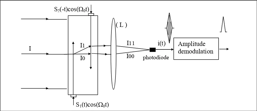
The principle of signal correlation is presented in Fig.1. The 2 signals are modulated by ultrasonic waves and are sent in opposing directions in a Bragg cell illuminated by coherent light. The product of the two signals is realized by two successive acousto-optic interactions [1]. The integration is realized by the output lens (L). The incident optical beam I will interact with the first signal s1 to yield a
modulated beam I1 and aresidual I0 . In their turn, I1 and I0 will , on interaction with s2, be splitted
respectively into I11,I10 and I01 and I00 .
The incident beam I is represented by its electric field vector: ) t 0 ( j
e k0.r
i A
2
t and r designate respectively the time and space coordinates.
The acoustic waves of frequency Ω0 and wavevector K are represented by :
) t 0 ( j 2 , 1 2
,
1 (t) S e
s = Ω ±K.z (2)
where S1,2=±1 (BPSK modulation). In relation with Fig. 1, one of the signals is time-reversed in order
to obtain correlation.
The AO interaction may be considered (at low efficiency) as a linear amplitude modulation associated with frequency and wavevector shifts equal to those of the acoustic waves.
Hence, for an efficiency α, the electric field of the fist diffracted beam is : k0 K).r
1 A
E =α j(ω0+Ω0)t−j( + 1 e
S (3)
The residual field is:
E0 = 1−α2Ei (4) The expression of all other field components are derived in the same manner. Particular interest is in the 2 parallel output beams having close frequencies :
E
00)E
iE
11 2j 0t 2E
00 21 2
e
)
t
(
S
)
t
(
S
and
1
(
−
α
=
α
=
Ω(5)
The detection is realized by the system (Lens + photodiode). The output current is :
(t) cos(2 t) S1(u)S2(u t)du C12(t)cos(2 0t)
L
0
0 − =Γ Ω
Ω Γ
=
∫
i (6)
[image:2.595.84.528.503.695.2]Where Γ is a constant factor and C12(t) designates the correlation of the two signals S1 ansd S2.
Figure 1 – The AO correlator.
Amplitude demodulation S2(-t)cos(Ω0t)
S1(t)cos(Ω0t)
I
( L )
I1 I0
I11
3
s(t)
3
The SS receiver
A view of the equivalent SS receiver diagram using an AOC is given in Fig. 1. The receiver role is to down-convert the received SS signal into baseband before performing correlation with a reference code. We distinguish the two filters of frequency responses H1(f) and H2(f) where :
1. filter H1(f) is proper to the AO correlator. It represents the acousto-optic interaction
frequency response and affects both the received and the reference signals. The equivalent normalized baseband representation of H1(f) is[3]:
)
∆f f sinc( (f)
H1 = (7)
Where
x ) x sin( ) x ( c sin
π π
= ,
f is the acoustic frequency, and ∆f is the cutoff frequency at –4dB corresponding to half the first-null bandwidth.
2. filter H2(f) is the receiver filter which characterizes the receiver channel. This filter affects the
received signal. Three different receiver filters are considered: ideal low-pass, RC filter and raised-cosine filter.
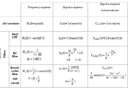
The characteristics of the AO correlator and the different receiver filters are given in Table1.
Figure 2 – The SS receiver
4
Analysis of the receiver performance
The received signal s(t) in Fig.1 consists of a desired signal Ac(t) corrupted by an additive zero-mean white Gaussian noise of power spectral density (PSD) equal to η :
s(t)=Ac(t)+n(t) (8)
where A is the amplitude of the received signal, n(t) denotes a sample function of the noise process.
At the receiver input the signal to noise ratio is:
η
σ
2 2 2 i
(SNR) A A
i =
= (9)
reference code
ideal correlator H2(f)
down converter antenna
receiver filter
H1(f)
H1(f) cf(t)
sff(t) output
4
Where
σ
i2 is the input noise power computed in a bandwidth equal to the chip rate which is, for convenience, normalized to one.The processing gain is defined as the enhancement obtained in the signal to noise ratio (SNR) as the signal goes through the receiver. In an ideal receiver (infinite bandwidth), the processing gain is equal to the spreading factor N i.e the number of chips in the code period [6]. When N is large, the autocorrelation of the code can be approximated by [6]:
Ccc(t)=tri(t) (10)
Where the chip rate is normalized to one and tri(t)=1-abs(t) for abs(t)<1 and 0 otherwise. At the receiver output, referring to Fig. 2, the signal obtained is:
i(t)=
N 1
[sff (t) *cf N
(-t)] (11)
where * is the convolution operator, the reference code is time–reversed in order to obtain correlation. The subscript (ff)refers to a two-stage filtering of signals: first in the receiver filter and second in the AO correlator. The subscript (f) refers to AO filtering alone. The superscript N refers to a single period of the code given by:
cN(t)=c(t)rect(
N t
) (12)
where rect(x)=1 for abs(x)<0.5 and 0 otherwise . Eq. (11) can be split as :
i(t) =
N 1
[Acff (t)+nff (t)]* cf N
(-t)
=
N A
[cff (t)* cf N
(-t)] +
N 1
[nff (t)* cf N
(-t)]
= s0(t)+n0(t) (13)
where s0(t) and n0(t) represent respectively signal and noise at the correlator output.
The signal to noise ratio (SNR)0 at the correlator output is defined as the ratio of the signal
correlation peak power
s
0(
0
)
2, at the coincidence instant, to the output noise varianceσ20[7] :2
0 2 0 0
) 0 ( )
(
σ
s
SNR = (14)
Using Eq.(4) and (9), the SNRE can be written as :
2 0 2 0
2 i 0
) 0 ( s A ) SNR (
) SNR ( SNRE
σ η =
= (15)
4.1 Signal and noise analysis
The detailed analysis of s0(t) and n0(t) is found in Ref. [4] and [5] .The expressions for s0(t) and
5
s0(t) = A [Ccc(t)*Ch1h1(t)*h2(t)] (16)
and ηC (t)*C (t)*C (t)*C (t) N
1 (t)
Cn0n0 = h1h1 h1h1 cc h2h2 (17)
where h1(t) and h2(t) are the impulse responses of the AO correlator and the receiver filter
respectively. Cxx(t) denotes the autocorrelation of x(t).
The output noise variance is given by the autocorrelation peak value Cn0n0(0) in Eq. (17).
4.2 Analysis of the correlator performance
The performance is studied in terms of two parameters:
1. the ratio α of the code chip rate (normalized to one) to the cutoff frequency ∆f of the AOC:
f 1 ∆ =
α (18)
2. the ratio β of the code chip rate to the receiver filter bandwidth.
4.2.1 Analytical results
Analytical results of the SNRE in the system are found in the case of ideal AOC : H1(f)=1.
Eqs. (11) and (12) reduce, in this case, to:
s0(t) = ACcc(t)* h2(t) (19)
and Cn0n0(t) = η/Ν [ Ccc(t)* Ch2h2(t)] (20)
The filter characteristics are given in Table 1.
The SNRE enhancement ratio is obtained from Eqs. 15, 19 and 20 as:
0 2
0 n 0 n
2
s
(
0
)
)
0
(
C
A
SNRE
==
η
(21)6
Figure 3 – SNRE loss in the receiver (ideal AOC)
4.2.2 Simulation results
Results in the general case (real AOC) are obtained from numerical simulation of the system (receiver + correlator) as defined in Fig. 2 and as described in Eqs. 16 and 17.
The value N has been taken equal to 1023 with 100 samples per chip. Results are presented in Fig. 4 for the three filters considered.
[image:6.595.195.420.92.284.2]We see that as α increases the curves become broader and the AOC filtering effects become dominant.
Figure 4 – SNRE losses (in dB) for different receiver filters: a) Ideal low-pass
b) RC filter
c) full roll-off rasied csosine β
α = 5
α = 0
α = 1
α = 2
α = 3
α = 0
α = 1
α = 2
α = 3
α = 5
β
α = 0
α = 1
α = 2
α = 3
α = 5
β
(a) (b) (c)
β
S
N
R
E
l
o
ss
(i
n
d
B
)
(1)
(2)
(3) (1): RC filter
(2): ideal low-pass
7
5
Conclusion
[image:7.595.29.531.276.622.2]The effects of different receiver filters on the processing gain in acousto-optic correlators are analyzed using a signal processing approach which is presented. Ideal, RC and full roll-off raised-cosine filters are considered. Analytical expressions are obtained for ideal correlators in terms of the ratio of the code rate to the filter bandwidth. In the general case, results are obtained from numerical simulation.
Table 1 –AO correlator and different receiver filter characteristics.
Frequency response Impulse response
Impulse-response
autocorrelation
AO correlator H1(f)=sinc(αf) h1(t)=(1/α)rect(t/α) Ch1h1(t)= (1/α) tri(t/α)
Ideal LPF H
2(f) = rect(βf/2) h2(t)= 2/βsinc(2t/β) Ch2h2 (t)=(2/β)sinc(2t/β)
R ec ei v er F il te rs RC filter ) RC 2 ( jf 1 1 ) f ( H2 π = β β + = 0 t 0 0 t e 2 ) t ( h t 2 2 < = ≥ β π = β π − t 2 2 h 2
h
(
t
)
e
C
β π −β
π
=
Raised-cosine filter (full roll-off) β 1 f 0 f)] β cos(π [1 2 1 (f) H2 < < += (1 x )
sinc(x) β
1 (t)
h2 2
− = (x = β 2t )
Ch2h2(t) =
8
6
Appendix
The analytical results derived in [4] and [5] for the different filters are here reported.
6.1 Ideal low-pass filter:
SNRE = N I(β) =
N
sin
c
(
f
)
df
/ 1 / 1 2
∫
β + β − (22)6.2 RC filter:
(23)
Where b=1/β and (24)
6.3 Raised-cosine filter:
) β 2π (π 1)Si 2 β ( ) β 2π Si(π 1) 2 β ( ) Si( β ) β 2π 2Si( 2π A (0) s0 − − + + + + π − = (25)
{
}
) β 2π Si(2π 2 1 ) β 2π Si(2π 2 1 ) β 2π (π 2)Si ( ) β 2π Si(π 2) ( ) Si( β ) Si(2 β ) β 2π 3Si( 4N (0) Cn0n0 − − β + + + β + − − β + + + β + π − π − π η = 2 (26)Where Si(x) denotes the Sine-Integral function:
dt
t
sin(t)
Si(x)
x 0∫
=
(27))]
1
e
(
b
1
1
b
)}
e
2
e
1
(
b
1
b
t
1
{
N
SNRE
b 2 2 bt ) 1 t ( b 2m m m
9
Acknowledgements
This work wassupported by the National Council for Scientific Research – Lebanon.
References
[1] N. J. Berg and J. N. Lee, Acousto-Optic signal processing, Dekker, New York, (1983).
[2] S. Kim, R. Narayanan, W. Zhou, and K. Wagner, “Time-integrating acousto-optic correlator for wideband random noise radar,”Proc. SPIE5557, 216-222, (2004).
[3] O. Bazzi, M.G. Gazalet, R. J. Torguet, J. M. Rouvaen and C. Bruneel, “Effects of acousto-optic correlator bandwidth on coded pulse compression,” Opt. Eng., 35(6),1656-1661 (1996).
[4] O. Bazzi, M. G. Gazalet, Y. Mohanna, A. Alaeddine, A. Hafiz, “Study of the effects of signal filtering on acousto-optic correlator performance”, Opt. Eng., 45(12), 128201, (2006).
[5] O. Bazzi, Y. Mohanna, F. Khalil and J. Assaad, “Effects of raised-cosine pulse shaping on processing gain in acousto-optic correlators”, Microwave and Optical Technology Letters, pp. 1558-1561, (2008).
[6] J. Proakis, Digital Communications, 4th ed., McGraw Hill, NY, (2001).