Detecting collusion on highway procurement

(1)

Económica, La Plata, Vol. LIX, Enero-Diciembre 2013 127

DETECTING COLLUSION ON HIGHWAY PROCUREMENT

M. FLORENCIA GABRIELLI

RESUMEN

Este trabajo se focaliza en el estudio de comportamientos cooperativos en mercados de subastas. Este artículo tiene dos objetivos principales. En primer lugar, desarrollar una metodología para detectar la presencia de cárteles usando el enfoque estructural. En segundo lugar, aplicar esta metodología a una base de datos de licitaciones para la construcción de carreteras en California. A través de la comparación de un modelo de competencia y un modelo de colusión se encuentra evidencia que sugiere que un subgrupo de firmas podría haber estado involucrado en un esquema colusivo.

Clasificación JEL: C14, C72, D44.

Palabras Clave: Subastas, Cartel, Enfoque Estructural, Colusión, Competencia.

ABSTRACT

This paper proposes a procedure to detect collusion in asymmetric first-price procurement. The main objective is twofold. First, to provide a methodology to detect collusion using a structural approach, and second to apply the methodology to field data on procurement auctions for highway construction in California. I identify two different sets of firms as potential ring members. Relying on an exogenous number of bidders and the assumption that within each type bidders are symmetric, I find evidence supporting the collusive scheme, for the two mentioned sets of firms by comparing a model of competition and a model of collusion.

JEL Classification: C14, C72, D44.

(2)

128 ECONÓMICA

DETECTING COLLUSION ON HIGHWAY PROCUREMENT

M. FLORENCIA GABRIELLI*

I. Introduction

Despite the vulnerability to bidder collusion, auctions and procurements are widely used mechanisms for allocating goods and services. Most government acquisitions are competitively procured (see Kelman, 1990). As Marshall and Meurer (2001) point out, construction and highway projects are typically procured by the government, assets of bankrupt businesses are usually liquidated by means of an auction, the federal government is the biggest auctioneer in the U.S. and offshore oil leases as well as timber from national forests are sold by means of auctions. There are several reasons why a good understanding of cooperative behavior in auctions or procurements is desired. The argument made most frequently in the literature is that collusion creates inefficiencies. In an auction context, the traditional view is that bidder collusion depresses seller revenue. In particular, in markets involving the government as a buyer or seller it is argued that collusion leads to increased government expenditures at procurements and decreased revenues at auctions. An additional problem in the case of the government is that raising government’s funds through distortionary taxes creates inefficiencies. Thus, the increased revenue spent in procurements because of collusion is not simply a wealth transfer.

Auctions are susceptible to bid rigging where bidders collude to dwarf the competition, thereby hurting the taxpayers. Bid rigging is pervasive in various markets, such as public construction, school milk supply, stamps; see Comanor and Schankerman (1976); Feinstein, Block, and Nold (1985); Lang and Rosenthal (1991); Porter and Zona (1993); Bajari (2001); Porter and Zona (1999); Pesendorfer (2000); Asker (2008); Harrington (2008) and municipal bonds among others. Marshall and Meurer (2001) argue that criminal and civil enforcement of the antitrust laws has deterred price–fixing in some market settings, but not bidder collusion. In particular they mention that many cases in the 1980’s and more recent high–profile cases serve as a reminder that the success of anti–collusive policies is limited in auction and procurement

(3)

DETECTING COLLUSION ON HIGHWAY PROCUREMENT 129

markets. Since bid rigging either lowers the revenue collected or increases the cost of procurement and if this shortfall were met through some distortionary taxes then it creates further inefficiencies. Thus, the increased revenue spent on procurements due to collusion is not simply a wealth transfer from taxpayer to the colluders. For example, in the case of United States of America v. Carollo, Goldberg and Grimm, the accused bidders are charged for rigging bids in many municipal bonds auctions cost state and local governments billions of dollars; see Taibbi (1986). It is important to detect and stop collusion as soon as possible.

Previous empirical work on collusion either rely on data from civil lawsuits to estimate the welfare cost of collusion or use reduced form estimation that ignores potential strategic interactions amongst colluders leading to misspecification errors.1_{It is not an exaggeration to say that such data from}

lawsuits are very hard to come by and even if they do, in most cases, it is already too late.

Identifying the characteristics of competitive behavior is a necessary first step towards collusion detection. Using the structural approach to analyze auction data, the main objective of this paper is to develop a methodology to detect collusive behavior. The idea is to compare two alternative models. Both models share the feature that bidders are allowed to be ex ante asymmetric (across types). As argued by Bajari (1997) and Bajari and Ye (2003), realistic models of bidding for procurement contracts should consider asymmetries among bidders. There are many sources that can create asymmetries among which the most important ones are location and capacity constraints. Other reasons often cited in the literature are different managerial skills, different information about the project, and the presence of a bidding ring, to name a few.

In this paper I identify two different sets of firms as potential ring members. Relying on an exogenous number of bidders and the assumption that within each type bidders are symmetric, I find evidence supporting the collusive scheme for the two mentioned sets of firms. This paper seeks to contribute to a better understanding of the implications of collusion. However I do not claim that this procedure can and should replace wiretapping and thorough criminal investigations. If anything, the procedure should be taken only as a first step in assessing the likelihood of bid rigging. On a technical ground, the paper also

(4)

130 ECONÓMICA

seeks to contribute to the literature on empirical auction pioneered by Guerre, Perrigne, and Vuong (2000) by expanding their testable implications of first-price auction models by including a model of collusion; see also Flambard and Perrigne (2006).

This paper is organized as follows. Section II outlines the theoretical model that leads to the econometric model. I first discuss the maintained assumptions throughout the paper. Then I present the theoretical framework that encompasses both, the competitive model and the collusive model. In this section I also provide some arguments for distinguishing the two competing models. Section III contains the econometric methodology followed in this paper. A description of the data and the market for construction projects in California is given in section VI. Section V shows how I classify different firms into different types of firms. In section VI I present the main results of this study and section VII concludes. Finally, an appendix collects some practical issues; in particular the choices of kernels and bandwidths used to estimate the models are discussed.

II. Structural analysis

In this section I describe the environment for a procurement model with private information in which firms compete for a construction project. Specifically I consider a first–price sealed–bid auction within the Independent Private Value (IPV) paradigm with asymmetric bidders and an exogenous number of bidders. First I discuss the assumptions maintained throughout the paper in the following section. Then, I introduce the case in which firms bid competitively and after that I adapt the model to allow for collusion.

II.1. Assumptions

(5)

Therefore, the number of bidders is exogenous. That is, firms do not make entry decisions on the basis of perceived profitability. Thus, the number of potential bidders, , and the number of actual bidders, , is the same. This implies that the reserve price is nonbinding. An announced binding reserve price, , or an entry fee, , are screening devices for participating in the auction. As pointed out by Perrigne and Vuong (1999) this complicates the nonparametric identification and estimation of the model.

There are few theoretical models in the literature which address endogenous entry decisions by means of a two–stage game (see e.g. Levin and Smith, 1994). However, in this kind of models the participation decision and the bidding decision of each firm are independent. This implies that in the second stage the bidding behavior is basically the same as the one described in this paper. To the best of my knowledge, there is no model in the literature considering a two–stage game in which both decisions are correlated. Thus, this is outside the scope of this paper.2

Let , and denote the number of participants for type 0, 1, and 2, respectively, which are observed by all firms. In other words, firm knows its actual competitors.

The distribution of private costs is given by . These three distributions are common knowledge with common support . Let denote the corresponding densities which are assumed to be continuously differentiable and bounded away from zero on their support.

II.2. Model for competitive bidding (Model A)

In the competitive framework, group 1 characterizes large firms that bid simultaneously (on a pairwise basis) more than a handful of times. Group 2 contains the remaining large firms and group 0 the other (small) bidders.3

Each firm of type submits a bid, , which depends on its own project cost . Firm maximizes its expected profit.

The expected profit of type bidders is:

2_{Recently some papers have taken endogenous participation into account, e.g.}_{Haile, Hong, and} Shum (2003); Marmer, Shneyerov, and Xu (2011); Krasnokutskaya and Seim (2011).

(6)

132 ECONÓMICA

( ) ( )

( )( [ ( )]) ( [ ( )]) ( )

where denotes type equilibrium strategy.

Lebrun (1996, 1999) and Maskin and Riley (2000a, b, 2003) among others, have studied the existence and uniqueness of the Bayesian–Nash equilibrium in asymmetric first–price, sealed–bid auctions.4_{It is known from this literature}

that the equilibrium strategies , and satisfy the following system of differential equations:

(1)

subject to the boundary conditions , and .5_{The above system of equations does not have a closed}

form solution, introducing a major difficulty for estimating the model. In this way, the application of direct estimation procedures to field data becomes cumbersome and only some numerical methods could be use but they require the numerical determination of the equilibrium strategies for any trial parameter value (see Perrigne and Vuong (1999, 2008) for further details).

To complete the specification of the econometric model that follows from the theoretical model, let be the distribution of bids corresponding to

4_{The assumptions about}

and described above guarantee that the type–specific equilibrium of this game exists and is unique.

(7)

bidders of type , and let denote the corresponding density. Following a similar argument to achieve identification as the one in Guerre, Perrigne, and Vuong (2000), system (1) above can be expressed as follows:

( )

(2)

This set of conditions establishes that unobserved private costs are identified from observed bids and bidders’ identities.

II.3. Model for efficient collusion (Model B)

The environment in which the collusive game takes place is similar to the one for the competitive model. That is, I assume that firms are engaged in a first–price sealed–bid auction where they compete for construction projects. The difference with the previous model arises in the way type 1 firms decide their bidding strategies.

In order to adapt the model developed above, I assume that the cartel behaves efficiently. This assumption can be justified if one thinks that there are side payments among ring members, a practice that has been used in cases in which collusion has been detected.6 I assume that side payments are cleared among all cartel firms before the target auction takes place. The cartel operates as follows; all ring members submit bids according to the strategy given by the first order conditions (see below). Moreover, the designated winner is the firm with the lowest cost. Hence, cartel members communicate before an auction is conducted to compare their cost estimates. Therefore the model in section II.2 can be adapted to this case. Thus, this model is a special case of the asymmetric IPV framework described above.

Under efficient collusion, both competitive firms and cartel firms participate in an auction. As before, there are 3 types of bidders. I label cartel firms as type 1 bidders. Large competitive firms are named as type 2 firms and

(8)

134 ECONÓMICA

small competitive (fringe firms) will be type 0 bidders. From the perspective of a type 1 bidder, there is only one such firm participating (seriously) in an auction. Hence, for this group of firms.7_{As before, there are} _and

bidders of type 0 and type 2, respectively. I maintain the assumption that bidders of type draw their private costs independently from a distribution

, .

I present now the maximization problem for each type of bidder and derive the first order conditions that private costs satisfy under a Bayes–Nash equilibrium. The expected profits for type bidders in this model are exactly as in the competitive case.

For type 1 bidders the expected profits under collusion are:

( ) ( )

Side payments are not included in the expected profits for type 1 bidders given that they are paid before the target auction whether or not the bidder wins (see above).

The first order conditions derived for type 0 and type 2 bidders are exactly the same as in the competitive model. For type 1 bidders, i.e. cartel members, only the minimum bid, can be rationalize by the FOC. After using a similar argument for identification as the one in Guerre, Perrigne, and Vuong (2000), type 1 costs can be expressed as follows:

(3)

Notice that under efficient collusion, expected profits, , are different only for type 1 bidders. Hence, the expression for private costs is also different for this type of bidders as compared to the competitive case. As mentioned above only the minimum bid is used for this type of players.

(9)

II.4. Comparing the two alternative models

As shown in sections II.2 and II.3, for each competing model there is an expression for private costs for each type of bidder (see equations (2) and (3)). Moreover, the difference between models boils down to the difference between type 1 costs in each case.

The idea now is to test whether the data are best explained by an Asymmetric IPV model in which there is no collusion (Model A), or by an Asymmetric IPV model in which type 1 bidders collude efficiently (Model B). To control for possible heterogeneity across auctions I consider the variable , , which denotes relevant characteristics of the project.8_{Therefore all the distributions are conditional distributions namely}

and . In particular, bid distributions depend on the number of bidders. I further assume that the vectors , are independent and identically distributed across .9

In order to be able to distinguish which of the two models described above best explains the behavior of bidders during the sample period considered, I rely on the following observation. The underlying distributions of private costs in the “right” model should not change with the number of bidders. This is a direct consequence of our exogeneity assumption. In other words, if it were the case that bidders are just asymmetric and therefore Model A is the appropriate one to use, then the underlying distributions of private costs for each type of bidder should be the same regardless of how many bidders participate in an auction when the competitive model is estimated. At the same time, under this scenario I expect to see more variation in cost distributions for the collusive model across . On the other hand, if type 1 bidders indeed act as an efficient cartel so that Model B is the relevant one to use, it must also be the case that the distributions of private costs do not change with the number of bidders and again some variation is expected for the competitive framework in this case.

The logic of the method is very simple and straightforward and relies heavily on the exogenous entry assumption as mentioned above. Suppose the true data generating process (DGP) is competition (Model A), then the conditional density of the recovered cost of bidders will be independent of the

(10)

136 ECONÓMICA

number of opponents, in other words, the recovered density should remain the same even when the number of actual bidders in each category changes. However, the estimated density under the misspecified model of collusion will be very sensitive to the number of bidders in each auction. This property is a direct consequence of exogenous entry assumption and is also symmetric because if the true DGP was collusion (Model B) then it would lower the competition faced by bidders from other type 1 bidders but the recovered cost distribution is still independent of the number of other bidders. But, under competition I expect the density to vary with the number of bidders.

I show that using this intuitive method a collusive model does rationalize the observed bids suggesting that the bidders (in the empirical application) might be colluding. The result of this method will be explained using the recovered conditional densities under various scenarios and the conclusion about the true DGP will be reached by way of “eyeballing” the figures (collected in the Appendix). Although the conclusion of this method is sensitive to the way bidders’ type are determined, because it affects the effective competition by affecting size of the collusive ring, the method can be used with all forms of auction data.

It is important to emphasize that failure to see unchanged cost distributions as the number of bidders varies could also be due to asymmetries within types. The model allows for asymmetric bidders across types, but symmetry is assumed for bidders of the same type. It is also possible that not all ring members are included in the group defining type 1 bidders. Moreover, other (non-identified) cartels could be operating during the sample period as well. If this were the case, then these firms would be (wrongly) labeled as type 0 or type 2 bidders thus yielding misleading results.

The method is based on structural estimation and does not require any prior knowledge about collusion but exploits the difference between the inverse bidding behavior with and without collusion, this is an advantage of this methodology with respect to reduced form analysis. Finally, the comparison of the models boils down to distinguishing between the cost distributions for type 1 bidders in each competing model.

(11)

In this section I outline the econometric strategy implemented to obtain the distribution of private costs for each subgroup. In the same spirit as Guerre, Perrigne, and Vuong (2000) I use a two step nonparametric procedure. In the first step I apply kernel methods to estimate the distribution and density of observed bids for each group of bidders. The second step then uses these estimated functions to recover pseudo private costs which are used to obtain the corresponding estimated densities.10

I first discuss some practical issues. The skewness of the bid distribution is a typical problem encountered with auction data. In addition, the use of kernel estimators is subject to the so_–called boundary effect so that some kind of trimming is often used.11 As a consequence it is common practice among empirical researchers to use a logarithmic transformation in order to keep a substantial number of observations after trimming (see for example [?]). For notational simplicity I suppress the dependence of the distributions on . Later, when presenting the estimators I include these variables explicitly. Applying the log transformation to system (2) yields:

( )

for j=0,2 and:

(4)

For system (3) the transformed system of equations differs from system (4) above only in the expression for , namely:

(5)

(12)

138 ECONÓMICA

where , is the cdf of and is its corresponding density, for . I abuse the notation and use to mean the lowest bid amongst type 1 bidders because under collusion the remaining bids are just cover bids and hence arbitrary. Henceforth, in estimating Model B, I shall always only use the lowest bid.

As noted earlier, some kind of trimming is often needed due to the bad behavior of kernel estimators close to the boundaries of the support of bids. In line with Guerre, Perrigne, and Vuong (2000) I adopt the following:

̂ {

for , and , where and are the minimum and maximum of log bids respectively, , are bandwidths and is the length of the support of the kernel.12

Let . Then, the hazard rate functions involved in the expressions for private costs given by the system of equations (4) and (5) can be written as follows:

for . Let denote the total number of observations for bidders of type . I consider auctions in which different types of bidders participate. Thus bidder , of type participates in auction . Relabeling bidders such that , i.e. the th bidder in auction , the sample consists of observation .13,14_{Thus, the estimators involved}

in the first step are:

12_{Without loss of generality I set}

.

13_{To keep the notation simple, I just include} _{in the formulas above. However, for the} computation of the estimator I have used , and separately.

(13)

̂ ∑

And

̂ ∑ ̂

With the sample of pseudo private costs _̂I estimate the cost densities in a second step as follows:

̂ ̂_̂

where

̂ ∑

and

̂ ∑

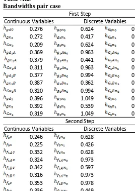
The functions and are kernels. The bandwidths for the continuous variables are denoted and . The bandwidths for the discrete variables are and The appendix discusses the choices of kernels and bandwidths.

(14)

140 ECONÓMICA

IV. Data description and awarding process

The California Department of Transportation (Caltrans) allocates construction projects using a First Price Sealed–Bid mechanism. The awarding process used by Caltrans is subject to Federal Acquisition Regulations and is therefore similar to other states’ procedures. This process is conducted in three steps: First, the Caltrans Headquarters Office Engineer announces a project that is going to be let and invites firms to submit bids. This corresponds to the Advertising Period, which lasts between 4 and 10 weeks depending on the size and complexity of the job. Second, potential bidders may submit sealed bids based on bid proposals that explain the project’s characteristics. Third, on the letting day, the bids received are opened and ranked. The project is awarded to the lowest bidder, provided that the firm fulfills certain responsibility criteria. After each letting, the information about all bids and their ranking is made public. The winning firm is awarded the job no more than 30 days after the letting date.

This section discusses the observable variables and provides descriptive statistics of the data. The sample consists of a subset of the Caltrans database on procurements of highway and road construction projects between January 2002 and January 2008.15_{During the sample period, Caltrans awarded 2,152}

contracts for a total of $7,645 million. The information available on every project awarded consists of the Bid Opening Date, Contract Number, Location, Number of Bidders, Number of Working Days, Engineers’ Estimate, Amount of the Bid and the Rank of the Bid for each of the bidding firms. Also there is information on the identity of each bidder and the address of the firm.16

In line with the theoretical model I only consider auctions in which at least 2 bidders participate and the winning bidder is the one with the lowest bid. There are 1,907 such projects, with a total of $6,989 million. A total of 823 firms submit bids on at least one of these 1,907 projects. The subset containing

(15)

big projects, which I define as those for which the engineers’ estimate is at least $1 million, has 438 bidders in 780 contracts awarded for a total of $6,502 million, 85% of the total. Given that the main purpose of this paper is to develop a methodology to detect potential collusive behavior, I restrict my attention further to big projects with engineers’ estimates ranging between $1 and $20 million. In this subset there are 724 projects and 413 bidders participating with 202 winning at least once. The total value of the winning bids is $2,408 million, which represents 31% of the total. I make a first classification of bidders on the basis of their revenue share in the sample. Thus, there are 25 firms with at least 1% revenue share. I call these firms Main Firms. In the theoretical model there are three types of firms. Thus, it is reasonable to think that potential cartel candidates are among the main firms. Although the exact nature of collusion and how it is sustained is not known, I think having subcontractors facilitates collusion as main bidders compete for the same subcontractors. This effect is more pronounced for the bidders who participate in several auctions and have some non–trivial market share, hence the 1% cutoff. Table 1 summarizes the bidding activity of these 25 (type 1 and type 2) bidders. All of the remaining bidders will be treated as type 0 fringe/small bidders.17

The first column in Table 1 gives the number of bids of each main firm. These bids represent 34% of all bids in the sample. The second and third columns show the number of times each main firm has won a contract and the “expected number” of wins, respectively. For example, firm A bids on a total of 50 projects against a varying number of firms, for, then expected number of wins is defined to be _∑ . By comparing these two columns it can be seen that with the exception of five firms, main firms tend to win more contracts than expected. In other words, this is suggesting that some firms win too often. The fourth column reports the average bid of each main firm in the sample and the fifth column the revenue share computed as the total value of the firm’s winning bid as a fraction of the total value of winning bids for all contracts. The last column in Table 1 contains the participation rate (i.e.

(16)

142 ECONÓMICA

the bid frequency rate). There is variation in this rate across firms with a remarkable 44% for firm D.

Table 2 provides summary statistics for a subset of variables in the sample. The mean number of bidders per project is above four with most of the contracts receiving between two and five bids. On average the winning bid is $3.33 million. This number is smaller than the average engineers’ estimate which is $3.77 million. The difference between the winning bid and the second lowest bid, “Money on the table”, reveals the existence of imperfect information among bidders. In the sample this difference is on average $300,000. The engineers’ estimate is highly positively correlated with bids (the correlation coefficient is 0.95). Despite this high correlation, it seems that the engineers’ estimate is not binding as a screening device since in 30% of the cases the winning bid is above the engineers’ estimate.

With the information in the database it is possible to construct measures of distance and backlog for each firm in each project. Distance is expressed in miles and refers to the distance between the location of each firm and that of the county where the project takes place. One would expect that closer firms have a cost advantage which should be reflected in bidding strategies. Even though there is a positive correlation between distance and bids in the sample, the magnitude of this correlation is small (0.012) suggesting that the location of the project does not influence bidding decisions much. The way the variable distance was constructed takes into account the longitudinal and latitudinal coordinates of the county where the project takes place and the coordinates corresponding to the zip code the firms have reported as their location. This variable is subject to measurement problems which could result in a low distance–bid correlation coefficient.

(17)

firm’s backlog at a given point in time; it is defined as the ratio of backlog to capacity.18

It is reasonable to expect that bidding rings would prefer to operate in markets with limited competition. Figure 1 below displays the distribution of the number of bidders per contract. The chart shows that most of the contracts have between two and five bidders with a peak at four. The fact that we see many few bidders is in line with the idea that competition is low in big projects. In general higher valued projects (between $1 million and $20 million as is the case in this application) attract relatively fewer bidders, suggesting that it is the main bidders who can gain the most by colluding and moreover, larger projects are more profitable, ceteris paribus.

V. Classifying bidders

Recall that according to the theoretical model there are three types of bidders. Here I explain how I classify participating firms as type 0, type 1 or type 2 bidders. The key point is to determine which firms are considered type 1 firms, since then the remaining main firms will be considered type 2 bidders and all other (small) firms will be treated as type 0 bidders. The natural candidates for type 1 bidders are the 25 main firms. I start by looking at the number of simultaneous bids among these main firms on a pairwise basis, I select those pairs with at least fifteen simultaneous bids as potential type 1 bidders. The result is fifteen pairs of firms involving fifteen main firms. Table 3 below shows the pairs selected. In the first column the total number of simultaneous bids submitted by each pair is reported. The second column gives the “expected” number of wins in those projects computed according to the level of competition in each one. These two columns together reveal that main firms participate (simultaneously with another candidate) more than expected. The next two columns contain the actual number of times the first member of the pair (third column) as well as the second (fourth column) wins a contract, respectively. Comparing the numbers in each of these columns to their expected counterparts in column two suggests that at least one member of the pair wins often which is in line with previous findings (see Table 1).

18

(18)

144 ECONÓMICA

A couple of interesting features arising from the comparison between Table 1 and Table 3 are worth mentioning. First, firm A bids almost exclusively against firm D. Second, firm E bids remarkably frequently with both firm A and firm D. This triplet of firms could be in principle one candidate. Also from Table 3 it can be seen that firms D and P (along with (A,D)) have the largest number of simultaneous bids. Due to availability of data for each pair, I concentrate especially on those with a large number of simultaneous bids; the pair (D,P) constitutes a candidate in this respect. To further investigate the behavior of these pairs of firms I follow Bajari and Ye (2003). These authors develop two conditions that must hold in equilibrium when bidding is competitive. The first condition states that conditional on observables, bids are independently distributed. The second condition refers to exchangeability of the bid distribution. As Bajari and Ye (2003) point out, these conditions may fail when bidding is collusive. In order to assess which pair of firms may be labeled as type 1 bidders I test for conditional independence and exchangeability.19,20

To test for independence I use a regression–based approach and consider the fifteen pairs of firms bidding frequently described above.21_{The model used}

is the following:

(6)

(7)

19_{This set of conditions is necessary for competitive bidding. However rejection does not imply} that bidding is collusive.

20_{Asymmetry amongst bidders can be attributed to their locations, carrying capacity,} informational differences and hence any realistic model of procurement auction should allow asymmetry, (Bajari, 2001; Bajari and Ye, 2003). Typically, only construction companies who participate mostly on highly valued project are called the regular bidders. It is important to note that using this test to narrow the set of potential colluders is just one possible way. For instance, Conley and Decarolis (2011) exploit some special features in Italian procurement data to identify the bidding rings.

(19)

where the regressors have been already discussed above. refers to the logarithm of distance and refers to the logarithm of the minimum of distances of all firms on project , excluding .

Thus, if firm is among the fifteen firms in Table 3, i.e. a main firm that frequently bids against another main firm, I use equation (6) with firm–varying coefficients. If firm is not one of the largest fifteen firms I use equation (7). For the estimation both equations are pooled and I include project fixed effects.

Let be the correlation between the residual to firm ’s bid function and firm ’s bid function, ̂ and ̂ , respectively. I use Pearson’s correlation test. Among all pairs, the null hypothesis of independence is rejected for all but one pair using a 5% two sided test.

Next, I test for exchangeability and, as before, I follow Bajari and Ye (2003) to construct two kinds of tests: Exchangeability at the Market Level by pooling the fifteen firms in one group and Exchangeability on a Pairwise basis. The null hypothesis of the test is: for all and for all

Let be the number of observations, the number of regressors and the number of constraint implied by . I consider the following statistic:

which is asymptotically distributed as F with parameters under the null hypothesis.

At the market level, the restricted model imposes that the effect of the four explanatory variables is the same for potential cartel members and the remaining firms (i.e. this is the exchangeability hypothesis). The null hypothesis of exchangeability is rejected when comparing the group of potential cartel members against the remaining bidders. Next, I conduct pairwise tests by pooling firms accordingly and find that the hypothesis of exchangeability is rejected at conventional levels for 13 out of 15 pairs including the pair (D,P) as well as (A,D) and (D,E).

(20)

146 ECONÓMICA

taking into account the number of simultaneous bids, firms D and P bid simultaneously more than a handful of times. Also, the triplet (A,D,E) is chosen as a potential cartel candidate. Therefore for the subsequent analysis I concentrate on two groups of candidates, namely the pair (D,P) and the triplet (A,D,E) as type 1 bidders.

V.1. Summary statistics for type 1 bidders

Firms D and P bid, on average, in projects of smaller size than the remaining thirteen large firms (i.e. type 2 bidders in the model) and roughly of the same size as the small firms (type 0 bidders). At least one of the firms participates in 325 projects winning 113 out of 724 contracts with and average winning bid of $3.67 million. On average the engineers’ estimate in these projects is above the winning bid. The average number of bidders participating in the 325 contracts is 4.65. Generally speaking, the data reveal that this pair tends to participate more often in small size projects with less competition. The other main firms tend to bid on larger projects and participate in 312 lettings. Type 0 bidders (i.e. the remaining smaller firms in the sample) participate in almost all auctions (666 out of 724). Table 4 below contains summary statistics per type when type 1 bidders are the pair (D,P).

Firms in the triplet (A,D,E) tend to bid also in smaller size projects relative to type 2 bidders. At least one of the firms participates in 329 projects winning 117 times. The average winning bid for this group is $3.70 million which is below the average of the engineers’ estimate. There are about five bidders participating in the projects where the triplet bids. Table 5 shows some summary statistics.

VI. Empirical results

(21)

include the same set of firms in each case (see Tables 4 and 5). Thus, there are two sets of results: one corresponding to the situation in which the firms (A,D,E) are type 1 bidders and the other to the case in which the firms (D,P) are type 1 bidders. I will refer to the former as the “triplet–case” and to the latter as the “pair–case”.22

There are both continuous and discrete variables involved in the estimation procedure. The set of continuous variables is given by the log of the bid for the th bidder in project and , the log of the engineers’ estimate in project .23_{For the discrete variables I include} _, _and _{, namely the number of}

bidders of type 0, 1 and 2 in each project.

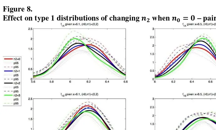
As discussed above, the main purpose is to determine which model best describes the bidding behavior of the different types of bidders considered in this analysis. Moreover, both the competitive model and the collusive model differ only in the underlying distribution of private costs for type 1 bidders. It is then natural to attempt to find differences across the models by looking at these two distributions. Inspection of the expressions for the costs for each type of bidder in each model (see equations (4) and (5)) reveals that one should expect to find the greatest differences when: both and are small and is large. A number of combinations among , and satisfy these conditions. I first discuss the results obtained from changing the number of bidders for types 0 and 2, respectively. The idea is then to assess the effect on type 1 distributions across models. I present results for two values of the (log) engineers’ estimate, namely 6.1 and 6.5. The first corresponds to fairly small projects (around $1.3 million). The second value is roughly the log of the average value in the sample.

Figures 2 and 3 below contain the estimated densities of private values for type 0 bidders in the triplet–case and the pair–case, respectively. The distribution of private costs for type 0 bidders exhibits some variation with respect to for both the triplet–case and the pair–case. The variability observed could be reflecting the randomness in the data. However, at least three other explanations are possible. First, the exogeneity assumption could be inappropriate for these firms. Second, it could be that there are asymmetries

22_{In all the figures presented below the dashed lines show 95% (bootstrapped) quantile of the} estimated distributions and the dotted lines represent 5% (bootstrapped) quantiles.

(22)

148 ECONÓMICA

across type 0 bidders, which are assumed away in the theoretical model. The case of endogenous entry would require one to explicitly include in the model a description of how firms decide whether or not to participate in an auction, which as discussed before is outside the scope of this paper. Finally, it could be that not all cartel members are captured in the group of type 1 bidders. It is most likely that the results found for type 0 bidders are a combination of the premises outlined above. Nevertheless, type 0 bidders are fringe firms which hardly ever win a contract.

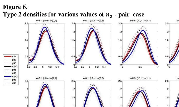
Type 2 bidders’ distributions do not show great variation for different values of . In Figures 4 and 5 I present the results for the triplet–case and in Figure 6 for the pair_–case. Unlike the case of type 0 bidders, these results are more in line with what one would expect if bidders are symmetric (within types) and the number of bidders is exogenous, as assumed in this paper. Moreover, even when there are type 0 bidders participating (see Figure 5 and second row of Figure 6), the distributions for type 2 bidders are remarkably similar.

In order to control for (to the greatest extent possible) other sources of variation, I decide to analyze how the distributions for type 1 bidders change as changes. This is mainly driven by the above considerations regarding how the distributions of type 0 and type 2 bidders behave when the number of bidders changes.

For the triplet–case, Figure 7 shows the effect on the distributions of type 1 bidders in the competitive model (Model A, see the first row) and in the collusive model (Model B, see the second row) when or and . The results for the case (not reported) are similar. The distribution of type 1 bidders shows less variation in the collusive setup. That is, under the exogeneity assumption and the assumption of symmetry within types, this piece of evidence suggests that firms (A,D,E) could be engaged in a collusive agreement.

(23)

and the pair–case could be driven by the fact that firm D is a type 1 bidder in both cases.

Overall, the evidence in the sample tends to favor the collusive model over the competitive model.

It is worth noting that I do not use a formal test, such as the Kolmogorov– Smirnov (KS) test, to distinguish between the two models. The main reason is that conducting this kind of test is not straightforward in this case. Recall that private costs are unobserved and I recover pseudo private costs, _̂, nonparametrically. Therefore a formal test should take into account the nuisance parameters introduced by the fact that _̂ is used instead of to estimate the distribution of private costs. This is not a trivial issue.24_Moreover,

the distribution of private costs obtained is conditional on the engineers’ estimate which is a continuous variable. This further complicates the formal comparison of the distributions of type 1 bidders across models. For the outlined reasons the KS test merits a separate paper.25

VII. Conclusions

This paper proposes a methodology to detect cartels acting in procurement– auctions. Two competing models within the asymmetric IPV paradigm are used to investigate the behavior of firms competing for construction projects. In the first model (Model A) firms are engaged in a competitive game. On the other hand, in the second model type 1 bidders behave cooperatively. The method is applied to field data on highway construction projects in California. Relying on the assumptions of an exogenous number of bidders and symmetry among firms of the same type (but not across types) I find evidence suggesting collusive behavior during the sample period analyzed. I acknowledge that some of my assumptions are strong. However even under this restricted framework I find evidence supporting the operation of cartels.

Relatively few empirical papers analyze the presence of bid–rings in auction markets within the structural approach. This paper contributes to this

(24)

150 ECONÓMICA

literature. The exogeneity assumption is restrictive. For instance it precludes endogenous entry. However, a model in which entry is endogenous leads to a number of challenges.

(25)

[image:25.595.55.403.129.513.2]

Table 1.

Revenue shares and participation of main firms

Note: Only firms with revenue shares >1% are reported.

Firm ID Number of _Bids Number of _wins

Exp. Number of

wins

Average bid (Mill. $)

Revenue Share

Participation rate

A 50 9 10.34 4.83 0.02 0.07

B 34 13 10.51 3.21 0.012 0.05

C 43 9 10.46 5.32 0.013 0.06

D 319 97 87.32 3.61 0.145 0.44

E 46 11 10.15 4.49 0.015 0.06

F 42 15 10.7 3.63 0.016 0.06

G 25 12 5.84 4.09 0.027 0.03

H 26 6 5.16 5.03 0.011 0.04

I 21 7 4.27 4.54 0.012 0.03

J 20 9 4.69 3.84 0.015 0.03

K 34 4 6.9 8.44 0.019 0.05

L 35 16 7.95 4.32 0.02 0.05

M 29 13 6.94 3.69 0.016 0.04

N 9 3 1.55 6.33 0.012 0.01

O 31 5 6.82 6.37 0.011 0.04

P 50 16 12.95 4.03 0.027 0.07

Q 33 9 6.31 3.35 0.017 0.05

R 28 10 8.1 3.48 0.012 0.04

S 47 12 8.82 4.37 0.021 0.06

T 25 13 5.99 3.75 0.021 0.03

U 68 16 15.22 4.77 0.026 0.09

V 26 7 4.78 5.75 0.025 0.04

W 41 11 7.18 2.92 0.019 0.06

X 41 7 10.27 4.5 0.021 0.06

Y 11 4 1.89 6.04 0.012 0.02

(26)

[image:26.595.56.367.131.281.2]

152 ECONÓMICA

Table 2.

Summary statistics

Note: All dollar figures are expressed in millions.

Table 3.

Simultaneous bids

No. observations Mean SD

No. Bidders 724 4.62 2.37

Winning bid 724 3.33 3.11

Money on the table 724 0.3 0.46

Engineers’ Estimate 724 3.77 3.49

All Bids 3347 3.79 3.51

Backlog 3347 4.3 9.76

Distance (miles) 3347 123.98 162.93

Capacity (across firms) 413 2.3 5.69

Utilization rate 3347 0.2 0.32

Firm Pair Simultaneous Bids

Expected Wins

First Bidder Wins

Second Bidder Wins

(A,D) 44 9.03 9 5

(A,E) 20 4.05 3 6

(B,D) 29 9.51 12 10

(C,D) 17 5.65 5 9

(D,E) 41 8.67 8 9

(D,F) 26 7.46 5 9

(D,H) 19 3.92 7 3

(D,I) 18 3.68 1 7

(D,O) 25 5.16 7 5

(D,P) 44 11.08 13 14

(D,R) 27 7.96 10 10

(D,V) 22 4.2 5 6

(D,W) 19 2.97 2 3

(M,X) 22 4.91 11 2

[image:26.595.58.362.327.571.2]

(27)

[image:27.595.59.401.127.375.2]

Table 4.

Summary statistics per type

Number of

observations Mean SD

Number of observations

Mean SD

No. Bidders 666 4.81 325 4.65 312 5.17

2.36 2.46 2.77

Winning bid 488 3.07 113 3.67 123 4.01

2.93 3.08 3.65

Money on the table 488 0.28 113 0.29 123 0.36

0.46 0.34 0.53

Engineers’ Estimate 666 3.64 325 3.74 312 4.32

3.38 3.27 3.72

All Bids 2520 3.69 369 3.66 458 4.41

3.49 3.18 3.81

Backlog 2520 1.37 369 24.6 458 4.05

3.4 16.44 6

Distance (miles) 2520 116.98 369 194.29 458 105.85

168.91 98.51 157.12

Capacity (across firms) 398 1.67 2 39.12 13 15.73

4.09 32.07 6.09

Utilization rate 2520 0.16 369 0.42 458 0.25

0.32 0.26 0.32

(28)

[image:28.595.59.400.126.375.2]

154 ECONÓMICA

Table 5.

Summary statistics per type

Figure 1.

Bidder concentration

Mean SD

Number of

observations Mean SD

No. Bidders 666 4.81 329 4.66 306 5.08

2.36 2.45 2.76

Winning bid 488 3.07 117 3.7 119 3.99

2.93 3.12 3.63

Money on the table 488 0.28 117 0.3 119 0.36

0.46 0.34 0.54

Engineers’ Estimate 666 3.64 329 3.76 306 4.35

3.38 3.34 3.77

All Bids 2520 3.69 415 3.85 412 4.3

3.49 3.34 3.75

Backlog 2520 1.37 415 22.75 412 3.62

3.4 16.64 5.39

Distance (miles) 2520 116.98 415 146.87 412 143.74

168.91 100.69 172.66

Capacity (across firms) 398 1.67 3 31.72 12 15.63

4.09 26.84 5.72

Utilization rate 2520 0.16 415 0.42 412 0.23

0.32 0.28 0.3

[image:28.595.53.388.400.574.2]

(29)

[image:29.595.56.399.118.321.2]

Figure 2.

Type 0 densities for various values of - triplet–case

Figure 3.

[image:29.595.49.406.147.565.2]

(30)

[image:30.595.56.401.115.321.2]

156 ECONÓMICA

Figure 4.

[image:30.595.54.402.347.550.2]

Type 2 densities for various values of and - triplet–case

Figure 5.

(31)

[image:31.595.54.402.113.321.2]

Figure 6.

[image:31.595.49.402.304.547.2]

Type 2 densities for various values of - pair–case

Figure 7.

(32)

[image:32.595.55.402.115.324.2]

158 ECONÓMICA

Figure 8.

[image:32.595.52.403.123.516.2]

Effect on type 1 distributions of changing when – pair-case

Figure 9.

(33)

References

Aryal, G., and M. F. Gabrielli (2012). “Estimating Revenue Under Collusion -Proof Auctions.” Working Paper, The Australian National University and Universidad Nacional de Cuyo.

Aryal, G., and M. F. Gabrielli (2013). “Testing for Collusion in Asymmetric First Price Auction.” International Journal of Industrial Organization, Vol.31: 26–35.

Asker, J. (2010). “A Study of the Internal Organisation of a Bidding Cartel.” American Economic Review, Vol. 3(100): 724-762.

Bajari, P. (1997). “The First Price Auction With Asymmetric Bidders: Theory and Applications.” University of Minnesota Ph.D. thesis.

Bajari, P. (2001). “Comparing Competition and Collusion: A Numerical Approach.” Economic Theory, Vol. 18: 187–205.

Bajari, P., and L. Ye (2003). “Deciding Between Competition and Collusion.” Review of Economics and Statistics, Vol. 85: 971–989.

Comanor, W. S., and M. A. Schankerman (1976). “Identical Bids and Cartel Behavior.” Bell Journal of Economics, Vol. 7: 281–286.

Conley, T. G., and F. Decarolis (2011). “Detecting Bidders Groups in Collusive Auctions.” Working Paper, University of Wisconsin, Madison. Esendorfer, M. (2000). “A Study of Collusion in First–Price Auctions.” Review of Economic Studies, Vol. 67: 381–411.

Feinstein, J. S., M. K. Block, and F. C. Nold (1985). “Asymmetric Information and Collusive Behavior in Auction Markets.” The American Economic Review, Vol. 75(3): 441–460.

Flambard, V., and I. Perrigne (2006). “Asymmetry In Procurement Auctions: Evidence From Snow Removal Contracts.” The Economic Journal, Vol. 116: 1014-1036.

(34)

160 ECONÓMICA

Haile, P., H. Hong, and M. Shum (2003). “Nonparametric Tests for Common Values In First-Price Sealed-Bid Auctions.” NBER Working Paper Series. Härdle, W. (1991). Smoothing Techniques with Implementation in. S. Springer-Verlag New York, Inc.

Harrington, J. E. (2008). “Detecting Cartels” in Handbook in Antitrust Economics, ed. by P. Buccirossi. MIT Press.

Kelman, S. (1990). Procurement and Public Management: The Fear of Discretion and the Quality of Public Performance. American Enterprise Institute Press.

Krasnokutskaya, E., and K. Seim (2011). “Bid Preference Programs and Participation in Highway Procurement Auctions.” American Economic Review, Vol. 101: 2653–2686.

Land, K., and R. W. Rosenthal (1991). “The Contractor’s Game.” The RAND Journal of Economics, Vol. 22: 329–338.

Lebrun, B. (1996). “Existence of an Equilibrium in First Price Auctions.” Economic Theory, Vol. 7: 421–443.

Lebrun, B. (1999). “First–Price Auction in the Asymmetric N Bidder Case.” International Economic Review, Vol. 40: 125–142.

Levin, D., and J. Smith (1994). “Equilibrium in Auctions with Entry.” American Economic Review, Vol. 84: 585–599.

Li, T., and I. Perrigne (2003). “Timber Sale Auctions with Random Reserve Prices.” The Review of Economics and Statistics. Vol. 85: 189–200.

Marmer, V., A. Shneyerov, and P. Xu (2011). “What Model for Entry in First -Price Auctions? A Nonparametric Approach.” Working Paper, University of British Columbia.

Marshall, R., and M. Meurer (2001). The Economics of Auctions and Bidder Collusion, Game Theory and Business Applications. Kluwer Academic Publishers, Norwell.

(35)

Maskin, E., and J. Riley (2000a). “Asymmetric Auctions.” Review of Economic Studies, Vol. 67: 413–438.

Maskin, E., and J. Riley (2000b). “Equilibrium in Sealed High Bid Auctions.” Review of Economic Studies, Vol. 67: 439–454.

Maskin, E., and J. Riley (2003). “Uniqueness of Equilibrium in Sealed High– Bid Auctions.” Games and Economic Behavior, Vol. 45: 395–409.

Perrigne, I., and Q. Vuong (1999). “Structural Econometrics of First-Price Auctions: A Survey of Methods.” Canadian Journal of Agricultural Economics, Vol. 47: 203_–223.

Perrigne, I., and Q. Vuong (2008). Auctions: Empirics. Palgrave McMillan, second edition.

Porter, R., and D. Zona (1993). “Detection of Bid–Rigging in Procurement Auctions._”Journal of Political Economy, Vol. 101: 518_–538.

Porter, R., and D. Zona (1999). “Ohio School Milk Markets: An Analysis of Bidding._”Rand Journal of Economics, Vol. 30: 263_–288.

(36)

162 ECONÓMICA

Appendix

Choices of Kernels and bandwidths

As it is well known in the nonparametric econometric literature, the choice of kernel is not crucial in practice. The estimators in this paper are multivariate kernels which are computed as the product of univariate kernels. That is:

where refers to the multivariate kernel, and denote the univariate kernels corresponding to the continuous variables A and B, say, and is the kernel for the discrete variables. Recall that .

The econometric procedure follows closely that of Guerre, Perrigne, and Vuong (2000). Accordingly, the kernels for continuous variables are required to be symmetric with bounded supports (see Assumption A3 in Guerre, Perrigne, and Vuong, 2000). Thus, I decide to use the triweight kernel function defined as for these variables, namely , and . The compact support of this function implies that only non-trimmed private costs are used in the second step to obtain the corresponding latent densities.

For the kernels involving discrete variables I use a Gaussian kernel. The main reason to change the kernel functions for the discrete variables has to do with the nature of these variables. That is, given that relatively small variation in the number of bidders it is desirable to give more weight to observations farther from the point at which estimation takes place. This is best achieved with a kernel with unbounded support.26

The smoothness of the distribution of private values is denoted by R, I assume R=1. The bandwidths' choice is critical in nonparametric estimation. To ensure the uniform consistency at the optimal convergence rates of the estimators the bandwidths for the continuous variables are of the following form:

(37)

̂ _, _̂ _, ̂ _, _̂ _. The constant term comes from the so-called rule of thumb and the factor 2.978 is the one corresponding to the use of triweight kernels instead of Gaussian kernels (see Härdle, 1991) and denotes the number of observations kept after trimming.

(38)

[image:38.595.53.326.128.511.2]

164 ECONÓMICA

Table A.1.

Bandwidths for the triplet-case

0.276 0.624 0.481

0.272 0.417 0.321

0.209 0.624 0.481

0.372 0.826 0.676

0.382 0.735 0.601

0.313 0.826 0.676

0.377 0.836 0.601

0.389 0.586 0.676

0.320 0.836 0.689

0.400 0.894 0.732

0.394 0.734 0.600

0.323 0.894 0.732

0.246 0.628

0.224 0.426

0.334 0.628

0.326 0.852

0.334 0.979

0.316 0.852

0.360 0.854

0.339 0.726

0.854 0.932 0.730 0.932 First Step

Continuous Variables Discrete Variables

Second Step

(39)

[image:39.595.53.321.129.506.2]

Table A.2.

Bandwidths pair case

0.276 0.624 0.481

0.272 0.417 0.321

0.209 0.624 0.481

0.369 0.963 0.791

0.379 0.441 0.362

0.311 0.963 0.791

0.377 0.994 0.820

0.387 0.362 0.298

0.320 0.994 0.820

0.396 1.049 0.856

0.392 0.539 0.439

0.319 1.049 0.856

0.246 0.628

0.225 0.426

0.332 0.628

0.324 0.973

0.342 0.597

0.316 0.973

0.353 0.978

0.336 0.449

0.978 1.086 0.548 1.086 First Step

Continuous Variables Discrete Variables

Second Step