How does dollarization affect real volatility and country risk?

Universidad Nacional de La Plata

Quintas Jornadas de Economía

Monetaria e Internacional

La Plata, 11 y 12 de mayo de 2000

How does dollarization affect real volatility and country risk?

Jorge Eduardo Carrera (CACES-UBA y UNLP),

Mariano Féliz (CACES-UBA, PIETTE-CONICET y UNLP) y

Demian Tupac Panigo (CACES-UBA, PIETTE-CONICET y

How does dollarization affect real volatility and country risk?

*

Jorge Eduardo Carrera1 (CACES-UBA, UNLP)

Mariano Féliz (CACES-UBA, PIETTE-CONICET, UNLP)

Demian Tupac Panigo (CACES-UBA, PIETTE-CONICET, UNLP)

Version: January/2000

Abstract

This study gives a non-traditional framework for the evaluation of the convenience of an asymmetric monetary association (such as dollarization), from the point of view of the country that gives up its monetary sovereignty.

In the analytical part we discuss the relationship between nominal volatility, real volatility and country risk. Given the social loss function of the policymaker, we determine the necessary conditions for dollarization to improve social welfare. With this in mind, we concentrate in the analysis of two main aspects: 1) the degree of synchronization existing between the cycle of the leader and associated country, and 2) the effect and relative importance of the different channels (the trade and financial channels) that transmit the shocks from the central country (the United States).

In the empirical part we perform an application of our analytical framework to the case of Argentina. To estimate the synchronization of the business cycles we use the coefficient of cyclical correlation, calculated for four different methodologies of de-trending. The effect and relative importance of the financial channel and the trade channel were extracted from the impulse-response functions and variance decompositions of a Vector Error Correction Model (VECM). We analyze the stability of the results altering the order of the variables, re-estimating the model with rolling sub-samples and modifying the deterministic component in the error correction mechanism.

As a general result dollarization in Argentina would not only reduce the risk of devaluation but also reduce the real volatility of the economy and so the country risk. For that reason, from the financial point of view the advantages of dollarization will depend on how much society values the alternative of keeping open the possibility of adjusting to extraordinary shocks with the exchange rate parity.

Keywords: monetary union, dollarization, VECM, risk, volatility, transmission channels, JEL codes: C5, F3

* _{The views expressed in this paper do not necessarily represent those of the institutions to which the authors belong. As usual,}

mistakes and omissions are the authors exclusive responsibility.

How does dollarization affect real volatility and country risk?

*

Jorge Eduardo Carrera1 (CACES-UBA, UNLP)

Mariano Féliz (CACES-UBA, PIETTE-CONICET, UNLP)

Demian Tupac Panigo (CACES-UBA, PIETTE-CONICET, UNLP)

Version: January/2000

Contents

1. INTRODUCTION...1

2. TRADITIONAL REQUISITES FOR A MONETARY UNION...2

3. COSTS AND BENEFITS OF DOLLARIZATION...2

4. DOLLARIZATION, NOMINAL VOLATILITY AND REAL VOLATILITY...4

5. VOLATILITY AND COUNTRY RISK...5

6. HOW DOES THE UNITED STATES’ CYCLE TRANSMIT IN THE CONTEXT OF AN ASYMMETRIC MONETARY UNION?...6

7. THE PROBLEM OF THE POLICYMAKER CONFRONTED WITH THE ALTERNATIVE OF DOLLARIZATION...8

8. DOLLARIZATION, REAL VOLATILITY AND COUNTRY RISK. AN APPLICATION TO THE CASE OF ARGENTINA...12

8.1. EFFECT AND RELATIVE IMPORTANCE OF THE DIFFERENT CHANNELS OF TRANSMISSION OF THE BUSINESS CYCLE. A VEC MODEL APPROACH...13

8.2. CORRELATION BETWEEN THE CYCLES...20

9. CONCLUSIONS...22

10. REFERENCES...24

11. APPENDIX...28

11.1. THE DATA: VARIABLES, SOURCE, FREQUENCY AND SAMPLE SIZE...28

11.2. RELATIONSHIP BETWEEN REAL VOLATILITY AND COUNTRY RISK (ARGENTINA)...29

11.3. RELATIONSHIP BETWEEN THE VARIABLES OF THE HYPOTHESIS IN EQUATIONS (2), (3), AND (5)...30

11.4. UNIT ROOT TESTS...31

11.5. TEST TO DETERMINE THE OPTIMAL LAG LENGTH FOR THE VEC MODEL...32

11.6. UNIT ROOT TEST FOR THE RESIDUAL FROM ERROR CORRECTION MECHANISM. ...33

11.7. SENSITIVITY ANALYSIS RESULTS. ...34

Keywords: dollarization, VECM, risk, volatility JEL classification codes: C5, F3

* _{The views expressed in this paper do not necessarily represent those of the institutions to which the authors belong. As usual,}

mistakes and omissions are the authors exclusive responsibility.

How does dollarization affect real volatility and country risk?

*

Jorge Eduardo Carrera1 (CACES-UBA, UNLP)

Mariano Féliz (CACES-UBA, PIETTE-CONICET, UNLP)

Demian Tupac Panigo (CACES-UBA, PIETTE-CONICET, UNLP)

Version: January/2000

1. Introduction

Dollarization is a key issue in the economic policy agenda of several emerging countries. After the crisis of the nineties, the discussion as regards the virtues of the different exchange rate regimes has reappeared. Nowadays, the alternative of dollarizing an economy2 has become extremely relevant, in academic as well as in political spheres. In Latin America the proposal has been discussed in general terms by a number of economists and even at an official level it has been presented and discussed by the President of Argentina's Central Bank (BCRA)3. At the same time, the Federal Reserve and a United States Senate committee have evaluated Argentina's proposal of a Treaty of Monetary Association. While some aspects of the discussion on the costs and benefits of dollarization relate to the contrast between flexible and fixed exchange rate regimes, a deeper analysis requires advancing in other aspects of a process of dollarization4.

Most of the studies on monetary unions have centered on the transmission of shocks through trade flows. On the contrary, the main objective of this paper is to concentrate on the financial aspects of a monetary association given the fact that, contrary to the experience of the 60s (when the optimal currency area theory was born), the freedom of capital movements of today has increased the importance of financial flows in the determination of the costs and benefits of dollarization.

For that reason we focus our analysis on the relationship between dollarization and volatility. We show how recent literature has attributed importance mainly to nominal volatility, like the case of excessive nominal volatility caused by central bank's discretionary policy (political shocks), or the nominal volatility needed for nominal contracts to work as a mechanism of hedging against economic shocks. We introduce the effects of real volatility and its direct influence on country risk. While dollarization directly reduces the risk of devaluation, its effects on the country risk are ambiguous. To make a precise statement with respect to the final effect of dollarization in financial terms, we must find out the sign and magnitude of its effect on the real volatility of the economy and thus on country risk.

In the analytical part of the paper we discuss the concepts of real and nominal volatility, the behavior of the channels of transmission of external shocks and the relationship between real volatility and country risk. We define the objective function of the policymaker and establish the necessary conditions for dollarization to reduce the aggregate risk (that is, the sum of devaluation risk plus country risk).

In the empirical section we apply this analytical framework to the case of Argentina. To estimate the association of the business cycles we use coefficients of cyclical correlation calculated from four different de-trending methodologies. The effect and relative magnitude of the financial and trade channels were extracted from the impulse-response functions and variance decompositions of a Vector Error Correction Model (VECM). We analyze the stability of the results altering the order of the variables, re-estimating the model with rolling sub-samples and changing the deterministic component in the error correction mechanism.

* _{The views expressed in this paper do not necessarily represent those of the institutions to which the authors belong. As usual,}

mistakes and omissions are the authors exclusive responsibility.

1 _{jcarrera@isis.unlp.edu.ar}

2 _{In general terms, dollarization can be understood as the resignation that a country makes of its monetary sovereignty to introduce the}

US dollar as its domestic currency.

3 _{Pou, P.(1999) "Más dolarización para profundizar la convertibilidad", Clarín 05/26/1999. Other Latin American countries, such as}

Ecuador, are discussion this alternative. See Roubistein (1999) for an approach favorable to dollarization and Posen (2000) for an analysis of the position of the United States on the issue.

4 _{The analytical part of this paper is also useful for the discussion of the case of "euroization" that is of interest in several European}

Finally, in the conclusions we combine the deductions of the analytical section with the results of the empirical part.

2. Traditional requisites for a monetary union

The dollarization of an economy can be understood as the conformation of a monetary union between a country that substitutes the US dollar for its domestic currency. The important characteristic of this type of union is that it is asymmetric, in the sense that there is a big country which acts as leader (the United States) while the rest of the countries (those opting for dollarization) act as followers5.

To analyze the effects of a process of dollarization it is useful to review the recommendations of the theory of optimum currency areas (OCA). If the countries fulfil the conditions for an OCA then they are able to optimally coordinate their economic policies. This theory initiated in the sixties with the works of Mundel (1961), McKinnon (1963) and Kenen (1969)6.

The traditional elements required to evaluate the optimality of a "monetary association" between two countries are:

1. The degree of similarity in their economic structures (Kenen criterion): the greater the degree of similarity in the structures, the greater the effects of external common shocks and the higher (and positive) the correlation between the business cycles.

2. The level of integration of the economies as measured by the volume of total trade between the countries (McKinnon criterion): the more integrated two nations are, the greater the transmission of shocks between them and thus, the more correlated their business cycles will be.

3. The existence of trade not based on comparative advantages: a high degree of intra-industrial trade will contribute to the equalization of the economic structures making shocks more similar.

4. Price and wage flexibility: the more rigid the nominal variables are, the most useful the exchange rate policy becomes as an instrument for changing relative prices7.

5. Mobility of factors of production such as labor and capital across countries or regions (Mundel criterion): the greater the mobility of factors in response to asymmetrical shocks, the greater the compensatory flows of factors will be (including migrations).

6. The existence of inter-jurisdictional fiscal transfers: this allows for countries to compensate for asymmetrical shocks with an instrument different from that of changing the bilateral exchange rate. The common argument in the traditional framework is that if shocks are similar (that is, if we find that the correlation of business cycles is positive, with similar intensity and duration), then using exchange rate policy (between partners) is not effective to compensate for shocks.

3. Costs and benefits of dollarization

To evaluate the specific impact of dollarization it is convenient to review synthetically the traditional view of the costs and benefits of a monetary union.

The benefits can be grouped, according to Fenton and Murray (1993), in four types: reducing transaction costs, reducing uncertainty, improving credibility and anti-inflationary discipline and improving the behavior of

5 _{The level of asymmetry is a characteristic that differentiates dollarization from the European Monetary Union (see Cohen and Wyploz,}

1990, or De Grawe, 1992). While in Europe the issue refers to the degree of marginal influence of each country in the decisions of a supra-national institution, in the case of dollarization it seems difficult to think about the incorporation of the countries, abandoning their domestic currencies, into the Board of the Federal Reserve Bank of the United States.

The are several papers that study the problem of monetary unions in the framework of game theory under a symmetric set up. However, only few do so in an asymmetrical context. Amongst these we find the work of Canzoneri, Henderson and Sweeney (1987) for a game between Europe and the United States, Cooper (1991) for an application of a Stackelberg solution and Carrera (1995) for the specific case of an asymmetric monetary union within a leader-follower framework.

6 _{In the nineties there has been a revalorization of this theory (for an analysis with recent developments see Masson and Taylor, 1991).}

In the theoretical aspects of the discussion Cassella (1993) gives microfundations to the OCA. Ghosh and Wolf (1994) have established a genetic approach to define its optimality and Mélitz (1991) has suggested an important theoretical reformulation. As regards the empirical aspects of the discussion Bini Smaghi and Vori (1993) study the European case and Chamie, DeSerres and Lalonde (1994), Bayoumi and Einchengreen (1992) and Rogoff (1991) study the case of NAFTA.

7 _{For shock asymmetry to be a problem, a certain price and wages inflexibility (especially downwards) is required. If domestic prices}

the monetary system.

Amongst the costs we find the loss of independence in macroeconomic policies and, consequently, the possible increase in real macroeconomic instability (due to the reduction in the number of instruments available to stabilize production, inflation or the current account). The importance of this loss will be determined by the weight of trade within the area (with respect to total trade) and by the degree of symmetry of shocks (Krugman, 1991)8.

The growing importance of the financial system in the determination of macroeconomic policies has created the need to redefine the costs and benefits of a monetary union, with a better understanding of some of the aspects already mentioned in the traditional view and incorporating some new ones of financial character. Blending the traditional view with the financial view (and remembering the asymmetry that exists in the case of a monetary union such as dollarization) we can put together a more accurate description of the costs and benefits of replacing the domestic currency by the dollar of the United States.

Benefits

A first benefit is the increased credibility of the monetary policy. When a country lacks such virtue it can import it delegating its monetary sovereignty to a "credible" partner that will guarantee a certain anti-inflationary discipline (Giavazzi y Giovannini, 1989; Carrarro y Giavazzi, 1990).

In association with this, we have the benefit of the reduction in the risk of devaluation. With the US dollar as the domestic currency, economic agents will no longer be in danger of suffering capital losses9.

Moreover, the reduction in the risk of devaluation implies a reduction in the cost of servicing the external debt (however, that the risk of devaluation is reduced with respect to the US dollar does not mean that the country risk disappears. The reason is that there is still the risk of default from the public sector as well as from the private one)

Additionally, if dollarization reduced the devaluation risk as well as the country risk, the domestic interest rate would fall, having a positive impact on investment, growth and perceived wealth (in this last case due to the reduction in the inter-temporal discount rate).

We should also stress the positive effect of dollarization on international trade between the United States and the associated country. By reducing transaction costs, dollarization induces increased trade in goods and services between the countries that do so in the same currency (Bergsten, 1999).

Costs

An important cost of dollarization is the reduction in the number of financial instruments available to hedge against real shocks since it implies the disappearance of nominal assets denominated in domestic currency (Helpman and Razin, 1982).

In addition, when opting for dollarization the country will periodically have to buy an important amount of dollars from the Federal Reserve to compensate for additional demand for money. In this situation the country cannot print domestic currency or gain interest on reserves10.

Furthermore, with dollarization foreign investors, which determine the country risk, know that there are no exchange instruments available to adjust relative prices and that public expenditure (in dollars) is mainly domestic payments and external debt payments (interest and capital, both in dollars). In a recession, to keep servicing its debt the government should reduce public sector expenditures in dollars or increase taxes. Thus, all of the adjustment will fall, in the short run, on fiscal measures. The perceived risk of fiscal default will increase. Also the probability that the government (having trouble to generate more revenues or reduce expenditures in dollars) will also be obliged to reduce its external debt payments will increase. In other words, dollarization would require a fiscal system even better than that of several US states since probably the associate country will not have access to the US Treasury's help through compensatory transfers, as the US states now do11.

8 _{Hit by a specific shock εif the country is dollarized and trades little with the United States (or with other countries with fixed exchange}

rate with the dollar), εwill be important in relationship with intra-area trade. In such a case, there will be a need for a great change in relative prices to compensate for the shock through trade within the area. If trade is important in relationship to ε, then the change in relative prices needed to compensate for the shock will be smaller.

9 _{Actually, only with respect to the dollar since there might be potential losses or gains with respect to other currencies.}

10 _{Levi Yeyati and Sturzenegger (1999) calculate that for the case of Argentina this senoriage is equivalent to 0.33% of GDP, assuming}

a growth rate of 5%, and inflation rate of 5% and a ratio circulating money/GDP of 3.4%.

11 _{Sachs and Sala-i-Martin (1991) found that in a negative shock any region of the United States gets a federal compensation of 30-40}

An additional specific cost would fall to the financial system which could no longer count on the Central Bank acting as a lender of last resort in a bank crisis (although potentially that role could be taken by the Federal Reserve or an ad-hoc Fund). This is not only a problem of tough and costly regulations. Even in the United States, where there are serious regulations, there have been crises where the Federal Reserve has had to intervene such as the case of the investment fund Long Term Capital (LTC) in 1998, or the crises of the regional banks in the eighties.

In those countries which now have a Currency Board regime there exists an extra cost from dollarization They would have to negotiate with the US government the loss of the interest in their international reserves now in deposit in the United States12.

Finally, another significant cost is the little importance that the United States places to its external sector in comparison with smaller countries. For that reason the dollar is allowed to fluctuate widely with respect to the Euro or Yen without the Federal Reserve or the Treasury expressing excessive preoccupation, contrary to the attitude of any small country which trades mainly with the rest of the world13.

4. Dollarization, nominal volatility and real volatility

In the analysis of the role of the exchange rate system there are two relevant factors that we wish to highlight 1) its effects on growth, and 2) its effects on the business cycle and the volatility of the economy.

With respect to the first aspect, the exchange rate regime is not a source of growth in the long run but it could reduce it if it generates excessive volatility of the economy. De Grawe (1988) shows how in a context of neoclassical growth with increasing returns to scale, it is possible that a reduction in exchange rate uncertainty, which reduces the interest rate, could increase the rate of growth. The adoption of a specific exchange rate regime could be used to: 1) reduce nominal uncertainty (or volatility), 2) control inflation (Calvo and Vegh, 1993; Fanelli and González Rozada, 1998), or 3) reduce real volatility14.

As it has been pointed out by Helpman and Razin (1982), changing from a monetary regime with a central bank to a monetary union implies a trade-off between the benefits of reducing excessive exchange rate volatility15 and the cost of reducing the number of financial assets available in the economy. With imperfect financial markets a flexible exchange rate regime is superior to a fixed exchange rate one because it increases the efficiency with which economic agents diversify risk (Helpman and Razin, op.cit.)16. A typical example of an instrument for hedging that is lost with a monetary union is the possibility of devaluation to adjust relative prices in response to shocks.

When policymakers have a propensity to generate policy shocks which are expected by the population there will exist an inflationary bias whose volatility could be influenced by short run electoral objectives; in such a case a monetary rule could be optimal. Neumeyer (1998) states that a monetary union is desirable when the gains from the elimination of excess volatility generated by policy shocks ("bad" nominal volatility) exceed the costs of reducing the number of instruments available to hedge against risk.

Our paper moves a step forward and complements the perspective of works already discussed by taking into account the problem of how an exchange rate regime (dollarization) affects the real volatility of the economy. We believe that the effects of dollarization on "good" and "bad" nominal volatility as well as on real volatility should be considered.

Behind this idea is the problem highlighted by Poole (1970) in his pioneering paper on what the most convenient regime to reduce real volatility is depending on the source of the shocks. If shocks come from the monetary market (they affect the LM curve) then the fixed exchange rate regime seems better, while if shocks originate in the goods market (affecting the IS curve) a flexible exchange rate regime would reduce

12 _{Dollars that would partially return to the country as circulating money}

13 _{For example, in the United States an important increase in productivity has occurred in recent years, which has induced a revaluation}

of the dollar with respect to the Mark (Euro) and the Yen. The country that wished to change its domestic currency for the dollar would have to at least equal the productivity performance of the United States to maintain its competitive capacity. Thus, dollarization implies importing external policy shocks (such as the greater US's real exchange rate volatility) not necessarily compatible with domestic preferences.

14 _{Since exchange rate changes (to modify relative prices) can help to absorb shocks in the presence of price rigidities or market}

imperfections (Roubini, 1999).

15 _{From the financial point of view we can make a distinction between "good" or "bad" nominal volatility of the exchange rate whether its}

origin is a "political" shock or a real shock (in preferences, in resources or in productivity). This last type of volatility is functional to the reallocation of factors and resources in an efficient way (Neumeyer, 1998).

16 _{An important assumption in this case is that there are adequate instruments for risk diversification within the countries but not}

the volatility of output.

From this section we can conclude that the effect of the exchange rate regime on real fluctuations is relevant for two motives. First, the greater the real volatility, the greater the domestic price changes the economy will require and, thus, the greater the advantages of a flexible exchange rate regime that admits certain nominal volatility ("good" volatility in the sense expressed by Helpman and Razin, 1982). In the second place, the greater the real volatility, the bigger the country risk implied in domestic assets. In the next section we discuss this last proposition in depth.

5. Volatility and country risk

When there are no restrictions on the mobility of capital and agents are neutral towards risk, the condition of uncovered interest rate parity has been widely used to evaluate the possibilities of arbitrage between different financial markets. Under these conditions any deviation is a white noise, unpredictable and of transitory character. Kaldor (1939) stated that in the activity of arbitrage it is necessary to allow for a risk premium that takes into account the problem of uncertain expectations and that more dispersion in expectations should imply a greater risk premium. In recent decades the importance of country risk to justify observed interest rate differentials between similar assets from different countries has been pointed out (Dooley, 1995). We can thus obtain the risk-adjusted interest parity condition17:

t e t

t

t

=

r

−

r

−

E

∆

e

−

u

*

δ

(1)

where δ is the difference in the interest rate between two assets of the same maturity and risk characteristics, r is the domestic interest rate, r* is the international interest rate,

E

∆

e

_eis the expected rate of devaluation and u is an IID random variable. Roubini (1999) states that the country risk (δ) can be interpreted as the risk of default of domestic assets.

Since the 1994 Mexican crisis and the successive Asian, Russian and Brazilian crises, in the case of the so called emerging countries, attention has been focussed on the role of the country risk in explaining the abrupt dismissal of exchange rate regimes and/or the recession that came with the process of absorption of negative shocks.

Some authors such as Calvo, Leiderman and Reihart (1993) and Calvo (1998) study the incidence of contagion effects on country risk. Others such as Avila (1998) and Rodríguez (1999) focus on the negative effect of country risk on the rate of change of output. However, what does not seem to have been analyzed with equal depth is the inverse relation. That is, what is the effect on the country risk of increased expected output volatility? For example, output volatility could be caused by growing efforts to reduce the nominal volatility with a rigid exchange rate regime (such as dollarization).

The relationship between volatility and country risk is highly intuitive: greater expected real volatility of output implies greater uncertainty as regards the profitability of investment and economic agents' consumption plans. This raises doubts as to the possibility of recovering invested capital or with respect to expected profits from holding domestic assets. Greater uncertainty will make agents require bigger returns from domestic assets in comparison with similar assets in countries with less real volatility.

To determine which theoretical position is the best answer to this problem, we check in the case of Argentina the relationship between the volatility of the business cycle and the country risk. Based on different econometric methodologies, we found that there exists a positive (and very significative) relationship between these variables, with increased volatility of the business cycle increasing the country risk18.

Based on these results we may state that the effect of dollarization on country risk (through its impact on real volatility) will depend on:

1) The exchange rate regime of the leader (in this case the United States) vis à vis the rest of the world. 2) The characteristics of the business cycle of the leader, since he is a source of shocks from which it is not

possible to insulate19.

17 _{Edwards (1999) applies a similar formula, that includes the equivalent rate when there are capital controls, for the discussion of}

equilibrium interest rates differentials.

18 _{In the section 2 of the appendix we present the results for cross-correlation coefficients and linear regression model between these}

variables.

19 _{The associated country could insulate from this shocks only with its fiscal policy. However, a country can use its fiscal policy if and}

In 1) the exchange rate regime of the United States could insulate the associated country (AC) from shocks from the rest of the world or generate additional shocks (i.e., the appreciation of the dollar caused by a shock of productivity in the USA would generate a change in relative prices in the AC).

In 2) it is stressed that the business cycle of the United States is a source of external shocks and depending on how fluctuations are transmitted they could amplify or reduce the cyclical volatility of the country associating with the dollar. To move forward in our analysis we concentrate on how fluctuations in the Unites States' output are transmitted and what effect they have on the country that associates as a follower in this asymmetric monetary union (dollarization).

6. How does the United States’ cycle transmit in the context of an asymmetric monetary union?

The business cycles of the different countries, understood as the variations of output around its trend, do not relate directly but through channels that transmit shocks from one economy to the other.

In the case of an asymmetric relationship big country-small country the transmission of the effects of the business cycle originated in the main economy to the different small countries occurs mainly through the transactions of goods (and services) and of financial assets (Canova and Ubide 1997; Schmitt-Grohé, 1998)20.

With the aim of simplifying the theoretical and empirical analysis, we may decompose the channels of transmission into two great groups: the financial channel and the trade channel.

The financial channel is related to the effects of the international interest rate on the level of capital flows to the emerging economies. This effect could be very significant as regards the size of fluctuations in the periphery for two reasons: 1) its determination is dominated by the economic conditions of the main center and thus they do not necessarily respond to the counter-cyclical needs of the emerging countries; 2) the high level of dependence on external savings by the emerging economies makes them very vulnerable to the perturbations in the international interest rate (Calvo, Leiderman and Reinhart, 1993).

In the trade channel, on the other hand, the effect of fluctuations in the business cycle of the leading economy (the United States) is transmitted through the movements in the trade flows (due to changes in quantities as well as in the terms of trade).

The relative size of each channel will indicate the magnitude of the effect on the economy hit by the shocks. If the channel has a very small magnitude in relationship to the economy under study, shocks coming through it will have only moderate effects on the cycle.

To summarize the previous analysis we present a simplified representation of the channels of transmission of cyclical fluctuations from USA to the AC (Figure 1)21.

20 _{For a survey on the correlation of the macroeconomic aggregates in the countries of the OECD see Blackburn and Ravn (1991) and}

Backus et at. (1992) for a presentation in the context of the Real Business Cycle theory.

21 _{The signs and relative importance of the different channels will be analyzed in the empirical section of the paper using vector error}

[image:10.612.144.440.54.380.2]

Figure 1 Channels of transmission of the United States' business cycle

GDP USA

GDP AC

i *

i Bilateral Trade

USA - AC

Balace Trade

AC-USA

Domestic Shocks

Domestic Shocks

Extra union trade shocks

Extra union finatial shocks

where AC is the country associated to the dollar, i is the interest rate that prevails in AC and i* is the interest rate determined by the Federal Reserve.

Each country suffers from domestic shocks but the small associated country also receives the influence of external shocks that are transmitted from the main center (the United States). The two channels of transmission are the financial channel (represented by the level of the United States interest rate) and the trade channel (represented by trade between the two countries)22. This effect can be decomposed into two stages represented by the complete lines: a) the impact of United States' imports and of the Federal Reserve's interest rate on trade from AC and on the interest rate of AC, respectively, and 2) the effect of this later variables on the GDP of the associated country.

From the perspective of AC, the economic intuition behind this simplified representation of analysis for the transmission of economic shocks is as follows: the United States' economy transmits its shocks through the trade channel and through the financial channel. When the USA's GDP is hit by a positive shock, two simultaneous processes begin: a) United States imports increase (affecting positively the GDP of AC through the trade channel), and b) the Federal Reserve increases the interest rate to slow down the economy to avoid over-heating (transmitting a shock through the financial channel that will affect negatively AC).

These hypotheses which refer to the mechanism of transmission of the business cycle may be formalized in the following expressions:

0

>

∂

∂

₋

USA AC USA

GDP

M

₍₂₎

0

*

_>

∂

∂

USA

GDP

i

₍₃₎

1

=

∂

∂

− − AC USA USA AC

M

X

₍₄₎

0

*

>

∂

∂

i

i

₍₅₎

0

>

∂

∂

−USA AC AC

X

GDP

₍₆₎

0

<

∂

∂

i

GDP

_{AC (7)}

where

X

_AC−USA represents exports from AC to the United States (symmetrically,

M

_USA−AC represents United States' imports coming from the country dollarizing its monetary system).

In section 2 of the appendix we present the econometric estimations and/or bibliographic references that provide empirical support for the hypothesis of equations (2), (3) and (5). Equation (4) derives from an accounting identity23, while the hypotheses contained in equations (6) and (7) will be confronted24 in the empirical section of the paper when we apply this analytical framework to the case of Argentina.

7. The problem of the policymaker confronted with the alternative of dollarization

The adoption of a more rigid exchange rate system such as dollarization could reduce real volatility if it acted as an automatic stabilization mechanism of the economy. This is a very important issue since a risk averse policymaker will prefer a more stable growth rate since this reduces the country risk perceived by (also risk averse) investors.

To make an evaluation of the aggregate effect of dollarization, we use a unified framework that takes into account the different effects (from the financial point of view) that are associated with this asymmetric monetary union. We want to specify which are the necessary conditions to ensure that dollarization will increase social welfare. We assume that the policymaker wants to minimize a social loss function that represents the external and financial fragility of the country (Fanelli and Gonzalez Rozada, 1998), where the control variable is the degree of rigidity of the exchange rate system (d).

[

RD

(

d

),

H

(

d

),

RP

(

_.

(

d

))

]

f

L

_d

=

σ

_GDPAC (Policymaker's social loss function) (8)

where RD(d) is the risk of devaluation, H(d) represents the number of financial instruments available to

compensate for (or cover against) real shocks to the economy (Helpman and Razin, 1982),

RP

(

σ

_GDP.AC

(

d

))

is the country risk (a positive function of the real volatility of domestic GDP) and d is a continuous variable representing the degree of rigidity of the exchange rate system25.

Differentiating the loss function with respect to d (under the assumption that, for example, this change takes the form of the conformation of an asymmetric monetary union such as dollarization) we obtain equation (9).

d

d

RP

f

d

H

f

d

RD

f

d

L

GDPAC

RP H RD

∂

∂

+

∂

∂

+

∂

∂

=

∂

∂

(

σ

_.

(

))

₍₉₎

We find that the result will depend, as we expected, on the assumptions (to be tested econometrically) made about the signs of the different coefficients.

With respect to the signs of the coefficients involved we assume that:

23 _{It is obvious that}

AC USA USA

AC

M

X

₋

=

₋ .

24 _{We will confront the hypotheses of equations (16) and (17) (to be presented in the following pages) which put together those in}

equations (4) and (6), and (5) and (7), respectively.

25 _{The sequence would be flexible exchange rate, "administered" or "crawling" exchange rate, flotation bands, traditional exchange rate}

0 > RD

f _{, (10)}

0

<

H

f

_{, (11)}

0 >

RP

f _{. (12)}

The sign of (10) is positive in as much as the social loss increases with the increase in the risk of devaluation. This risk characterizes the "bad" volatility that is related to the inflationary bias of the system when there is a discretionary monetary policy.

With respect to (11) its sign depends on the results from Helpman and Razin (1982) where a greater number of nominal financial instruments reduces the social loss since it allows for better risk diversification by allowing the fluctuations in the exchange rate that act as an instrument for the diversification of real risk. Finally, equation (12) implies that, as with the risk of devaluation, the social loss increases when the country risk increases.

With respect to the rest of the partial derivatives from the different sources of social loss involved with respect to dollarization, we assume the following signs:

0 < ∂ ∂ d RD ₍₁₃₎ 0 < ∂ ∂ d H ₍₁₄₎

0

.

))

(

(

) / ( . ) ( . .

<

=

>

∂

∂

∂

∂

=

∂

∂

− + +

d

RP

d

d

RP

_GDPAC

AC GDP AC GDP

σ

σ

σ

(15)

In (13) we state that a movement towards a more rigid exchange rate regime such as dollarization reduces the space for independent policies by the central bank thus eliminating the risk of devaluation26. In equation (14) we simply indicate that dollarization reduces the set of available nominal financial instruments in the economy.

The central point in our analytical framework relates to the sign of equation (15) that will determine the final result of equation (9). The central problem is to determine the effect of dollarization on the country risk. To find this result we need to remember our previous discussion on how the United States' business cycle is transmitted through the financial channel (FC) and the trade channel (TC). Combining equations (4) and (6) we obtained the expected effect of a shock transmitted through the trade channel on the associated country's GDP:

0

>

∂

∂

−AC USA AC

M

GDP

₍₁₆₎

In a similar fashion, combining (5) and (7) we may find the expression that summarizes the effect of the financial channel on AC's GDP27:

0

*

<

∂

∂

i

GDP

AC (17)

Without loss of generality we present a functional form in which real volatility

σ

_GDP.AC depends on the relationship between the business cycles of the United States and the associated country, and the relative importance of each channel. Thus we have the following expression:

26 _{Levi Yeyati and Sturzenegger (1999) show that even dollarization could be reversed. They state certain conditions under which there}

are perverse incentives for the policymaker in a country that is receiving the dollars it needs to substitute its domestic money supply (sharing the benefits of senioriage). They show that under certain conditions, the policymaker may renounce the compromise and reinstate the domestic currency. However, this seems more a case of theoretical importance than of practical significance given the high punitive power of an agent such as the Federal Reserve.

            +

= GDP_ACUSA

FC FC FC TC TC TC AC GDP IMP IMP VDS IMP IMP VDS g

d . /

. ρ

∂

∂σ ₍₁₈₎

with

g

′

>

0

g

´´<

0

where g is a monotonically increasing (at decreasing rates) function in the argument, VDSTC and VDSFC

indicate, respectively, the participation of the trade channel and the financial channel in the volatility of AC's product, IMPi represents the effect of each channel in the product of AC (thus, the ratio IMPi/|IMPi| with i=

(FC, TC) allows us to obtain the sign of the effect of a change in the variable that represents each channel of transmission28) and

USA AC

GDP /

ρ

indicates the correlation between the cycle of AC's GDP and the cycle of United States' GDP29.

Assuming the hypothesis of equations (2), (3), (16) and (17), equation (18) implies that:

1) In the case of the trade channel (TC), when the two economies are in an expansionary phase of the cycle (outputs are positively correlated), an increase in the demand in the United States produces an increase in exports from AC towards the USA. Since exports are a component of aggregate demand this works as an additional external positive impulse that gives an additional pull to the business cycle in AC. In this case the trade channel increases real volatility. On the contrary, if the cycles are negatively correlated, when AC is in a downward phase of the cycle the United States is expanding. In this case an increase in external demand for goods from the United States implies an increase in exports from AC and, thus, a positive impulse in its GDP. In this case the trade channel reduces real volatility.

2) With respect to the financial channel, let us assume that the two economies were positively correlated and both expanding. In this case the increase in the interest rate by the Federal Reserve to avoid over-heating the USA's economy would produce a similar effect in the economy of AC30. In this way, the cycle would be contained, reducing the range of fluctuation of the growth rates in AC. On the contrary, if the two economies were negatively correlated, that is when the United States is growing the associated country is in recession, the increase in the Federal Reserve's rate would increase the downturn in the AC's economy.

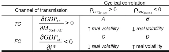
Table 1 resumes the previous discussion. With synchronized cycles (

USA AC

GDP /

[image:13.612.161.437.445.530.2]

ρ

>0) the financial channel (FC) reduces the volatility of the cycle and the trade channel (TC) increases it. On the contrary, with cycles negatively correlated, the FC increases real volatility and the TC reduces it.

Table 1 Change in the volatility of AC GDP

Cyclical correlation

Channel of transmission 0

/U S A> AC GDP

ρ 0

/U S A< AC GDP

ρ

TC >0

∂ ∂ −AC USA AC M GDP A

↑ real volatility

B

↓ real volatility

FC

₀

*

<

∂

∂

i

GDP

_AC C

↓ real volatility

D

↑real volatility

From this framework of analysis we may establish the following two propositions: Proposition 1:

Assuming the usual mechanisms for the transmission of the business cycle in a center-periphery framework31, dollarization will reduce real volatility and thus the country risk if and only if the following conditions are fulfilled: a) if correlation between business cycles is

28 _{By dividing the value of the coefficient by its absolute value we exclusively keep the sign which is adequate since our objective is to}

isolate the result from the size of the effect.

29 _VDS

T C and VDSFC will be proxied in the empirical section by the proportion of the variance of the output of AC that is explained by the

trade and financial channel, respectively. The values for IMPT C e IMPFC will be obtained from the responses of AC's output to a shock in

the trade and financial channel, respectively. Finally,

U S A AC GDP /

ρ will be proxied through different estimations for the coefficient of cyclical correlation between the United States' and AC's output.

30 _{For an analysis of the negative association between the United States' interest rate and the level of activity in Latin American}

countries see Calvo, Leiderman and Reinhart (1993), Frenkel (1998), and Roubini (1999).

31 _{Hypotheses contained in equations (2), (3), (16) and (17) which will be checked and ratified in the empirical section and in section 3 of}

positive, the financial channel should dominate the trade channel. b) if the correlation between the cycles is negative, the trade channel should dominate the financial one.

In terms of equation (18) we have the following alternatives when we combine the possible results for each of the free variables of the equation32:

0

/

>

>

FC AC USA

TC

VDS

and

VDS

ρ

(19)

0

/

>

<

FC AC USA

TC

VDS

and

VDS

ρ

(20)

0

/

<

>

FC AC USA

TC

VDS

and

VDS

ρ

(21)

0

/

<

<

FC AC USA

TC

VDS

and

VDS

ρ

(22)

FC TC VDS

VDS = (23)

0

/USA

=

AC

ρ

(24)

In the case of expressions (19) and (22), dollarization will increase the real volatility of the GDP of AC (

_σ

_GDP.AC).

If, on the contrary, we verify that the cyclical behavior and the relative importance of the different channels correspond to expressions (20) or (21), dollarization will allow the associated country to import a monetary policy that will act as an automatic stabilizer of its economy, reducing

AC GDP.

σ

.

Finally, if the channels have the same relative importance (equation 23) or if cyclical correlation is not significantly different from 0 (equation 24), then dollarization induces no effect on the associated country's real volatility.

The economic intuition in proposition 1 can be presented clearly through the following two examples: Case A (equation 19)

If both countries were in recession when their cycles are synchronized (

ρ

_AC/USA

>

0

) and the trade channel

dominates the financial channel (VDSTC > VDSFC), the fall in exports of AC to the United States (due to

reduced USA's demand) would accentuate AC's domestic recession. Since the financial channel is of little importance the counter-cyclical policy that the Federal Reserve could be practicing in the United States would not be enough to compensate the volatility amplifying effect of the trade channel. In this case, dollarization implies resigning an instrument (such as the exchange rate policy) that could act as a stabilizer of the business cycle reducing real volatility.

Case B (equation 22)

If the United States' economy is expanding while AC's economy is in recession, the increase in the demand for AC's exports could smooth AC's recession. However, since the financial channel dominates, the counter-cyclical policy of the Federal Reserve increases the downturn in AC (since AC's interest rates will have to increase there too). Once again, dollarization implies losing the possibility of using a domestic counter-cyclical policy either to practice expansive policies or to compensate for the increase in the Federal Reserve's rate.

The economic intuition behind the other alternatives (equations 20, 21, 23 and 24) can be easily derived from the previous examples.

Proposition 2:

Dollarization will improve social welfare if the weight given by the policymaker (society) to the reduction in the aggregate risk (devaluation risk plus country risk) is greater than the loss of social welfare due to the reduction in the number of available instruments to cover for risk.

32 _{It is important to remember that from the assumptions in equations (16) and (17), we already know the results for IMP}

T C (positive) and

IMPFC (negative), so that the only free variables are VDST C, VDSFC and

U S A AC GDP /

43 42 1 4 4 4 4 4 3 4 4 4 4 4 2 1 4 4 3 4 4 2 1 ) ( ) ( ) ( ) / ( ) / ( . ) ( . ) ( ) ( ) ( ) ( 0 − − − − + − + + + + − +

∂

∂

∂

∂

_<−

          ∂ ∂ ∂ ∂ + < ∂ ∂

d

H

f

f

d

RD

f

_H D RP RP RD si d

L GDPAC

AC GDP

σ σ

(25)

The intuition is that given a certain level of loss due to the disappearance of an instrument for hedging the greater the reduction in the country risk, the smaller the reduction needed in the devaluation risk for dollarization to be welfare improving.

This framework for the analysis of the net benefits of dollarization is sufficiently general to be applied to the different countries. In the second part of this paper we find the signs and dimensions corresponding to the case of Argentina, focusing the analysis on the relationship dollarization - real volatility - country risk.

8. Dollarization, real volatility and country risk. An application to the case of Argentina

In this section we develop an empirical application of the analytical framework presented in the previous sections to assess the potential impact of dollarization on the real volatility of Argentina’s economy.

The selection of Argentina as a case of study relates to the fact that, in this country, dollarization has been subject to intense debate in political as well as academic spheres lately33. Moreover, the president of Argentina's Central Bank has presented an official proposal to implement a Treaty of Monetary Association with the United States (Pou, 1999). The interest of certain Argentine economists in implementing dollarization relates to the lack of credibility of Argentina's monetary policy, as a result of years of excessive exchange rate volatility and inflation rates that reached the 200% monthly.

In 1989 the first (constitutional) presidential succession in four decades occurred, in the midst of an unprecedented economic crisis, the most significant manifestation of the crisis was hyperinflation.

After a number of stabilization plans failed in the early nineties, the government relied on a radical solution to the fiscal problem and fixed the exchange rate as a means to stop inflation. But the government needed an instrument that would help it gain credibility. Besides the fixation of the exchange rate, Argentina established, by law, a compromise not to devaluate the currency and to fully back the money base with its hard currency reserves (Convertibility law, a currency board regime). As a mechanism for coordinating expectations and reducing inertial inflation, indexing of wages and prices was prohibited. In addition the reduction of trade restrictions was used as a price control mechanism for tradable goods34.

The implementation of these policies was complemented with others of structural character such as privatization of public services and State reform (reduction in the number of public sector workers, decentralization of basic services, etc.).

After 9 years of virtually null inflation and strong growth, the marginal benefits of these policies seem to be fading out. In relationship with the exchange rate regime, there are disputes between those who propose the devaluation of the exchange rate to compensate for a number of recent negative real shocks and those who believe that the right direction is exactly the opposite, that is to go deeper into the Convertibility, dollarizing the economy.

For these motives, the analysis of the impact of dollarization on the real volatility of the Argentinean economy constitutes an empirical application of great relevance to the decisions of economic policy that relate to the monetary system of this country.

The empirical analysis consists of two stages. First, we present a vector error correction model (VECM) to examine the effect and relative importance of the trade and financial channels in Argentina.

Second, we examine the correlation between the business cycle of Argentina and the cycle of the United States. The objective of this second part is to obtain an appropriate estimation of the coefficients of cyclical correlation to determine (together with the effects and relative importance of the different channels) the impact of dollarization on social welfare through its effect on country risk (which is a positive function of real volatility).

33 _{Other Latin American countries have been discussing the subject lately. For example, several working papers from researchers at the}

Central Bank of Costa Rica take into account the idea of dollarization in Costa Rica seriously (see for example Ramos et at, 1999). Recently, Ecuador's government has announced the intention of abandoning the Sucre, their local currency, in favor of the US dollar. The idea resulted in tremendous upheaval (which included a failed coup-de-etat) within the country.

34 _{Few countries in the world have a regime such as this, amongst them (besides Argentina) Hong Kong, Estonia, Lithuania and Brunei.}

8.1. Effect and relative importance of the different channels of transmission of the business cycle. A VEC model approach

Following the traditional methodology to analyze the structure of the different shocks that hit the economy35, we build the vector error correcting model (VECM) to describe the way in which shocks are transmitted from the United States to Argentina36.

VAR models are used in the prediction of the series included in them and for the identification of the different kinds of shock, affecting the economies.

Our work makes use of the two tools derived from VAR models: impulse-response functions and variance decomposition procedure.

To use the impulse-response functions and the variance decomposition procedure it is necessary to identify the shocks for each and every variable in the system. In more general terms, n(n-1)/2 restrictions are needed to exactly identify the model (where n is the number of variables in the model).

For that purpose, one methodology that provides these restrictions is the Cholesky decomposition which imposes that the matrix A(0) (which incorporates the contemporaneous effects of the variables) be triangular inferior37.

Different authors have criticized the arbitrary methodology of imposing restrictions of identification on the Cholesky decomposition, indicating, for example, that the results in most cases (when there is correlation amongst the residuals of the equations) are very sensitive to the order in which the variables are included38. Alternative solutions have appeared. Using the general structure of the VAR models, changes are introduced in the identification restrictions. Among them, the developments by Blanchard and Quah (1989) and Johansen (1991, 1995) stand out using long run restrictions to identify the different models.

However, there are noticeable differences as regards the reasons why restrictions are introduced in each methodology. While Blanchard and Quah (based on the supposition of a vertical aggregate supply curve in the long run) determine that demand shocks will not last, Johansen’s methodology takes the long run restrictions from the data generating process without imposing ad-hoc behavioral restrictions on the different markets.

In this paper we use Cholesky decomposition to find short run identification restrictions39 and Johansen’s methodology to estimate long run relationships without having to impose a priori restrictions.

The structure of the model can be easily explained through the following example of a VEC with n variables and one lag for each variable40.

Let:

t t

t

z

z

=

Γ

_{1 −1}

+

ε

(26)

where

z

_t= the (nx1) vector

[

z

1t

,

z

2t

,

z

3t

,

z

4t

,...

,

z

nt

]

of variables in the model

t

ε

= the (nx1) vector

[

ε

1_t

,

ε

2_t

,

ε

3_t

,

ε

4_t

,...

,

ε

_nt

]

of gaussian errors

1

Γ =an (nxn) matrix of parameters.

Subtracting

z

_t−1 from each side of (26) and letting I be an (nxn) identity matrix, we get,

t t

t

I

z

z

=

−

−

Γ

+

ε

∆

(

1

)

₋1 , or

t t

t

z

z

=

π

+

ε

∆

−1 (27)

35 _{See Sims (1980), Blanchard and Quah (1989), Johansen and Juselius (1992), and Amisano and Giannini (1997) for theoretical and}

empirical applications in which VAR or VEC models are used to identify the different shocks hitting an economy.

36 _{In recent years there has been a great number of papers which study the transmission of the international business cycle using VAR}

modeling for the empirical analysis. Amongst the most interesting papers in this field of research we recommend: Calvo, Leirdeman and Reinhart (1993), Chamie, DeSerres and Lalonde (1994), Canova (1995a), Horvath, Kandil and Sharma (1996), and Schimitt-Grohé (1998).

37 _{For further detail see Hamilton (1994).} 38 _{See Enders (1995).}

39 _{Knowing that under this kind of decomposition the identification of shocks is very sensitivity to the order in which the variables are}

included in the model, we also develop a sensitivity analysis for the results that includes 6 different orderings for the variables.

where

π

is the (nxn) matrix

−

(

I

−

Γ

1

)

_t and

π

ij denotes the element in row i and column j of

π

.

If each

ij

π

is equal to 0, the rank of the matrix

π

is 0 and (27) is equivalent to an n-variable unrestricted VAR in first differences.

On the other extreme if

π

is of full rank the long run solution to the system is given by the n independent equations:

0

.

.

.

.

.

.

.

.

.

.

.

.

.

.

.

.

.

.

0

0

3 3 2 2 1 1 2 3 23 2 22 1 21 1 3 13 2 12 1 11

=

+

+

+

+

=

+

+

+

+

=

+

+

+

+

nt nn t n t n t n nt n t t t nt n t t t

z

z

z

z

z

z

z

z

z

z

z

z

π

π

π

π

π

π

π

π

π

π

π

π

L

L

L

In this case none of the series has a unit root, and the VAR may be specified in terms of the levels of all of the series.

If there are r<n vectors of cointegration, the VAR should be re-expressed in first differences with the inclusion of the r independent error correction mechanisms that establish the long run relationships between the variables.

Assuming that r=1, each sequence

{ }

z

_it can be written in error correction form. For example, we may write

t

z

1

∆

as: t nt n t t t

t

z

z

z

z

z

₁

=

π

_{11 1 1}

+

π

_{12 2 1}

+

π

_{13 3 1}

+

+

π

_{1 1}

+

ε

₁

∆

− − −

L

−

or, normalizing with respect to

z

_1t−1:

t nt n t t t

t

z

z

z

z

z

1

=

α

1

(

1 1

+

β

12 2 1

+

β

13 3 1

+

+

β

1 1

)

+

ε

1

∆

_{− − −}

L

₋ (28)

where

α

₁ determines the speed of adjustment to a long run dis-equilibrium, while the

β

_1i give us the coefficients which determine the long run relationship.

These results remain unchanged if we formulate a more general model by introducing the lagged first differences of each variable into each equation. In such fashion we obtain the following expression that includes the n equations of the model (assuming that there exists only one vector of cointegration, that is r=1): t n i k j j it ij nt n t t t i

it

z

z

z

z

z

z

₁ 1 1 1 1 1 3 13 1 2 12 1 1

)

(

β

β

β

ψ

ε

α

∑∑

= = − − − − −

+

+

+

+

+

∆

+

=

∆

L

(29)

where

ψ

_ij is a (nx1) vector of parameters for equation i and lag j.

Equation (29) represents a VEC model with n variables, one cointegrating vector and k lags for the variables in first differences.

We will use this type of VECM to evaluate the effect and relative importance of the financial and trade channels in the transmission of the business cycle from the United States to Argentina.

Next we present the main characteristics of the model and later on we show the most important results. The model

We develop a vector error correction model with three variables41 (Federal Reserve Interest Rate (FEDRATE), imports of the United States from Argentina (IMPOUA)42 and the Industrial Production Index of Argentina (IPIARG)), and an intercept in each equation.

The variables are in logs, seasonally adjusted43 and in first differences44. FEDRATE and IMPOUA represent the financial and trade channels respectively45.

The IPIARG is taken as an approximation of Argentine GDP. As we can see in the section 1 of the appendix, we use the Industrial Production Index instead of the actual GDP because there are no reliable estimations for Argentina’s GDP on a monthly basis and because the correlation coefficients between these variables is extremely high.

The model is thus defined as follows:

t t t i t k

i i

t z z

z = Ψ∆ +Π +µ +ε

∆ _{− −}

=

∑

1

1

. .

. (30)

where

1 − t

z

= the (3x1) vector

[

FEDRATEt₋,IMPOUAt₋₁,IPIARGt₋₁

]

,

t

z

∆

= the (3x1) vector

_[

_]

t t

t IMPOUA IPIARG

FEDRATE ∆ ∆

∆ , , ,

t

ε

= the (3x1) vector

[

ε

_1t

,

ε

_2t

,

ε

_3t

]

of uncorrelated, homocedastic, gaussian errors,

t

µ

= the (3x1) vector of the deterministic components,

i

Ψ

=an (3x3) matrix of parameters, and

Π

is the (3x3) matrix of rank r (to be tested) which contains the parameters of the cointegrating vectors.

The next step consists in verifying the conformity of the model with the data generating process evaluating the order of integration of each variable, the rank of

Π

and the optimal lag length.

Unit root test

For each variable (in levels and in first differences) in the model we perform the ADF (Dickey and Fuller, 1979)46 and Phillips-Perron (1988)47 tests to detect the presence of unit roots in the series48.

In table 7 in section 4 of the appendix we present the results of the different tests for a confidence level of 95%.

We verify that almost all variables are I (1) (integrated of first order). There is a certain contradiction for the variable IPIARG49. However, the results that indicate that the series is I (1) seem more robust since 83% of the tests for this variable (5 out of 6 different specifications for the ADF test and the Phillips-Perron test) state that its data generating process would be correctly represented by a random walk.

Since every variable can be considered I (1) we fulfill the first necessary condition for the construction of a VECM50. The second necessary requisite to build the model is that the rank of the matrix of the cointegrating vectors should be greater that 0 (zero) and less than n. For our model the rank of the matrix should be equal to 1 or 2.

Tests for the optimal lag length.

According to Canova (1995a) "the trade-off between over-parametrization and oversimplification is at the heart of the selection criteria designed to choose the lag length ".

There are different selection criteria to determine the optimal number of lags in VEC models. In this paper we use some of the more traditional such a Akaike criterion (Akaike, 1973), Schwarz criterion (Schwarz, 1978)

43 _{Through X-11 ARIMA method. For further details see section 1 of the appendix.}

44 _{It is convenient to remember that in the error correction mechanism(s) the variables appear in levels and lagged one period.} 45 _{In section 1 of the appendix we present the reasons for the sample period and for the variables included in the model. Also, we show}

the characteristics of the series (periodicity, transformations, etc.), the econometric software used (and the procedures) and the source of the information for each variable.

46 _{The number of optimal lags for each specification was obtained following Akaike criterion (Akaike,1973).} 47 _{For this test we take the truncation lag recommended by Newey - West (1994) for monthly series.}

48 _{We checked the following three specification for the deterministic component in both tests: 1) unrestricted, which includes time trend}

and intercept, 2) idem 1, but without the time trend, and 3) restricted, without any deterministic component.

49 _{Even when the variable is I (1) for almost all specifications (5 out of 6) for the ADF test as well as for Phillips-Perron test, when we}

include the time trend and the intercept in the equation, the Phiillips-Perron test indicates that the series is I (0).

50 _{Recently, Pessaran et al. (1999) have proposed a new approximation to test the existence of long run relationships that is}