A phenotypic analysis of three population-based metaheuristics

(1)

A Phenotypic Analysis of Three Population-based

Metaheuristics

Alina Orellana - Gabriela Minetti

Laboratorio de Investigaci´on en Sistemas Inteligentes Universidad Nacional de La Pampa

Rep´ublica Argentina

Abstract

Metaheuristics are used as very good optimization methods and they imitate natural, biologic, social and cultural process. In this work, we evaluate and compare three different metaheuristics which are population-based: Genetic Algorithms, CHC and Scatter Search. They work with a set of solutions in contrast to trajectory-based metaheuristics which use an only solution. From a comparative analysis, we can infer that Genetic Algorithms and CHC algorithms can solve satisfactorily problems with a growing complexity. While Scatter Search provides high quality solutions but its computational effort is very high too.

Keywords: Metaheuristic, Genetic Algorithms, CHC, Sccatter Search.

1 INTRODUCTION

In the last 50 years, many methods have been developed to solve combinatorial optimization problems. The Simplex is used to optimize linear functions, the random searches, the dynamic programming, the brunch and bound methods, among others, are used to solve nonlinear functions. But these techniques are not enough to solve problems belonging to NP-complete problem class and with a growing complexity. To mitigate this weakness, the metaheuristics are used. A metaheuristic is a method with a high abstraction level that can analyze big search spaces, keeping an equilibrium between diversification and intensification of the search. Besides it provides very good results although those solutions can not be optimal.

The diversification term is associated with the exploration of whole search space, while the intensification is related with the exploitation of a specific area from the search space. The equilibrium degree between these two aspects determines how efficient and efficacy the search is.

(2)

to a set of solutions; the most used of them are: Genetic Algorithms(GA) [12], CHC algorithm [4], Scatter Search (SS) [8], Path Relinking (PR) [10], Particle Swarm Optimization (PSO) [22] and Ant Colony Optimization (ACO) [16].

Many works present how some metaheuristics solved a specific problem but they only explain the metaheuristic behaviour for that particular problem. Our objective is to analyze different population-based metaheuristics (GA, CHC, SS) considering four optimization functions, which represent many combinatorial optimization problem. We try to provide empirical evidence for the practical usefulness of those metaheuristics.

The rest of this article is organized as follows. The next section introduces the optimization functions used to test the population-based metaheuristics. Section 3 shows the three meta-heuristics used in this work: GA, CHC and SS. Section 4 shows the experiments performed and discusses the results of those experiments. Finally, the last section concludes and provides hints on further research.

2 TEST FUNCTIONS

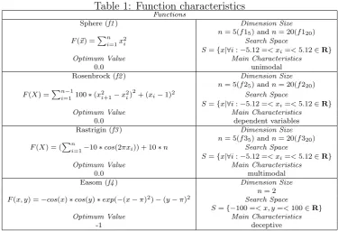
[image:2.595.109.485.428.684.2]

In this paper, we use four different optimization functions to analyze the above mentioned metaheuristics; they are: Sphere function (f1), Rosenbrock function (f2), Rastrigin function (f3), Easom function (f4). Those functions have been chosen since they represent real problems and belong to a function set which is used to study many optimization methods [13]. All these functions are mapped in Rn_→_{R. The characteristics of each function are shown in Table 1.}

Table 1: Function characteristics

Functions

Sphere (f1) Dimension Size

n= 5(f15) andn= 20(f120)

F(~x) =Pni=1x 2

i Search Space

S={x|∀i:−5.12 =< xi=<5.12∈R_}

Optimum Value Main Characteristics

0.0 unimodal

Rosenbrock (f2) Dimension Size

n= 5(f25) andn= 20(f220)

F(X) =Pni=1−1100∗(x 2

i+1−x 2

i)

2

+ (xi−1)2 _{Search Space}

S={x|∀i:−5.12 =< xi=<5.12∈R_}

0.0 dependent variables

Rastrigin (f3) Dimension Size

n= 5(f35) andn= 20(f320)

F(X) = (Pn_i₌₁−10∗cos(2πxi)) + 10∗n Search Space

S={x|∀i:−5.12 =< xi=<5.12∈R_}

0.0 multimodal

Easom (f4) Dimension Size

n= 2 F(x, y) =−cos(x)∗cos(y)∗exp(−(x−π)2₎₋₍_y₋_π₎2 _{Search Space}

S={−100 =< x, y=<100∈R_}

-1 deceptive

3 POPULATION-BASED METAHEURISTICS

Generally, the metaheuristics can be classified as trajectory methods (single-point search) or

(3)

Genetic algorithms, CHC algorithm and Scatter Search algorithm belong to the population-based methods.

In general the problem search space is codified as binary strings, each string represents a solution (or chromosome for GAs). We use a binary vector as solution to represent real values of the variable. The string length depends on the required precision, in this work the decimal part has six places. For example, the domain of such variable of f1 has a length 10.24; which means each variable range has be divided into at least 10.24∗1000000 equal parts. This means that 24 bits are necessary for each variable and a chromosome with 24∗n bits is required to codify af1 solution. Specifically forf15, f25 and f35 the chromosome size is 120, forf120, f220

and f320 is 480 and for f42 is 56.

For mapping a binary string (b23, b22...b0) into a real number x is done in two steps.

• Convert a binary string from base 2 to base 10

(b23, b22...b0)2 = ( 23

X

i=0

bi∗2i)10=x

′

(1)

donde bi representa el valor de un alelo

• Find a real number belonging to a respective range

x=−5.12 +x′ ∗(10.24/(224−1)) (2)

where -5.12 is the left boundary and 10.24 is the length of the domain

3.1 Genetic Algorithms

Genetic Algorithms (GAs) [12], a special class of Evolutionary Algorithms (EAs), are computer-based solving systems, which use evolutionary computational models as a key element in their design. They have a conceptual base simulating the evolution of individual structures via the Darwinian natural selection process [6]. GAs have been applied to a wide variety of problems from pipeline engineering, VLSI circuit layout, resource scheduling, machine learning, bioinfor-matics problems [14, 15, 19, 20], among others.

As it is shown in Algorithm 1, a GA maintains a population of multiple tentative solutions (individuals) which evolve throughout generations by reproduction of the fittest ones. Selection, recombination, and mutation are the main operators used for modifying individual features. So, it is expected that evolved generations provide better and better individuals (tentative solutions in the problem space).

(4)

Algorithm 1Genetic Algorithm

t = 0;{t is the generation number}

initialize P(t);{P(t) is the population at generation t}

evaluate individuals in P(t);

while _{not condition} do t=t + 1;

selectC(t) fromP(t−1)

apply variation operators (recombine and/or mutate) to individuals inC(t) building C′₍_t_);

evaluate individuals inC′(t);

replace some individuals in P(t−1) withC′(t) to build P(t);

end while

rest of the population) and as a result the population diversity is lost. On the other hand, with a low selection pressure, the diversity is kept.

The crossover operation tries to combine good characteristics from different parents selected in order to yield a new individual. Then this kind of operators is merely explorative. After all, their goal is to create variation. The main idea is the crossovers ability to combine and/or disrupting pieces of information. That is strongly related with the increment and reduction of diversity in the population. The n-point crossover randomly chooses n crossover points and cuts the two parents of length L into n + 1 segments (the same points in both parents). After that, it creates the first child putting together the odd segments from the first parent and the even segments from the second one. The second child is created by taking the opposite decisions.

A further generalization of n-points crossover is the uniform crossover [23, 25]. For each bit in child1, uniform crossover decides (with some probability p) which parent will contribute its value in that position. The second child would receive the bit from the other parent.

3.2 CHC Algorithm

CHC (Cross generational elitist selection, Heterogeneous recombination, and Cataclysmic mu-tation) is an evolutionay algorithm proposed by Eshelman in 1991 [4]. This method is a GA which objective is to reach an equilibrium between diversity and convergence using: an elitist selection, a variant of uniform crossover, an incest prevention way and a restart method. The pseudocode of CHC is presented in the Algorithm 2.

CHC randomly chooses two parents to recombine if the Hamming distance between them is greater than a certain threshold (d); that is known as incest prevention and allows to slow the pace of convergence. This method guarantees that only the most diverse potential parents are crossed over and the diversity requirement is automatically decremented as the population converges.

The crossover operator used to recombine those couples of parents is a variant of the Uniform crossover (HUX). This operator crosses over half the non coincident bits, where the alleles to be exchanged are chosen at random without replacement. In this way the Hamming distance between parents and offsprings is maximum and the chance to combine good schemata from both parents in a child is incremented, but, all schemata of the same order have an equal chance of being disrupted or preserved.

(5)

The use of HUX and incest prevention in conjunction preserve a number of diverse chro-mosomes, but they do not guarantee to avoid a premature convergence. Being necessary some mutation mechanism. However, a traditional mutation is not effective in CHC. For that a new mechanism was created, Restarts, this process reinits a part of population when such population does not diverge.

Algorithm 2CHC Algorithm

t = 0;{t is the generation number}

d= L/4;{d is the threshold value and L is the chromosomoe size}

initialize P(t);{P(t) is the population at generation t}

evaluate individuals in P(t);

while _{not stop condition}do t=t + 1;

selectC(t) fromP(t−1)

recombine structures inC(t) building C′(t); evaluate individuals inC′₍_t_);

selectP(t) from C′₍_t_{) and} _P₍_t₋_1);

if _P₍_t_{) =}_P₍_t₋₁₎then d=d−1;

end if

if _{d <}₀ then

diverge P(t);

d=r×(1.0−r)×L;{r is the divergence rate} end if

end while

3.3 Scatter Search Algorithm

The Scatter Search methodology was first introduced by Fred Glover in 1977 [8] as a heuristic for integer programming, based on strategies to combine decision rules. After that, Manuel Laguna had been made many extensive contributions [17]. This metaheuristic belongs to the family of Evolutionary Algorithms, since they are based on combination of a solution set. Although the main difference with respect to GAs, is the way to generate the initial solutions. The GAs generate randomly the initial population and SS uses a systematic strategy to create the first solutions.

SS starts generating a set P of diverse solutions, where each solution is subjected to an improvement method. FromP is selected a subset called Reference Set (RefSet), which is used in the search process. From this RefSet, parents subsets are generated. The individuals of each subset are combined obtaining one or more offsprings. After that, an improvement process is applied over each offspring and finally they are considered to update the RefSet (see Algorithm 3). SS uses an evolutionary process which involves five methods:

• Diversification Generation Method. This method generates a collection, P, of diverse solutions, using one or more seed solutions as an input.

• Improvement Method. Usually, this method is a local search which tries to transform a solution into an enhanced solution.

(6)

• Subset Generation Method. This procedure operates on the reference set producing sub-sets of its solutions as a basis to combine solutions.

• Solution Combination Method. Given a subset of solutions produced by the Subset Gen-eration Method, this method produces one or more combined solutions. Although this method is analogous to the crossover operator in genetic algorithms but it can combine two or more solutions.

Algorithm 3Scatter Search Algorithm

Start with P =⊘;

while ₍_|_P _|6₌_{P size}₎do

X=Diversif icationGeneration();

X′ =Improvement(X);

if _NOT(_X′ _∈_P₎then P =P∪X′;

end if end while

SetRef =Ref erenceSetU pdate(build, P);

OrderSetRef according to their objective function value;{where the best overall solution is first on the list}

while _{(not stop condition)}do

P arentSubsets=SubsetGenration(SetRef);

while_{P arentSubsets}₆₌_⊘do

X =SolutionCombination(P arentSubsets);

X′ =Improvement(X);

if ₍_f₍_X′ _{< f}₍_X₎_{andN OT}₍_X′ _∈_SetRef₎₎then SetRef = Ref erenceSetU pdate(update, X′);

reorderSetRef;

end if end while end while

4 COMPUTATIONAL EXPERIMENTS

In this section the behavior of each above describe metaheuristic algorithm is analyzed us-ing the test functions (presented in Section 2): Sphere function (f1), Rosenbrock function (f2), Rastrigin function (f3) and Easom function (f4). For each metaheuristic, different parametric settings are considered; besides their results and analysis are presented. These algorithms were executed under MALLBA software [26], which was created by research group from Malaga, La Laguna and Barcelona Universities. For each algorithmic setting we have performed 30 independent runs per function and we use an Intel Centrino duo processor with 1.73 Ghz and 1 GB of RAM.

We use the following relevant performance variables to analyze the behavior of each algorithm:

(7)

– AOT (Average Optimum Time). It is the average time that the algorithm takes to find the optimal value.

– ATT (Average Total Time). It is an average of the total time consumed by each algorithm per execution

– AOI (Average Optimum Iterations). It is an average of the iteration (or generation) number which is necessary to find the optimum.

4.1 Genetic Algorithm

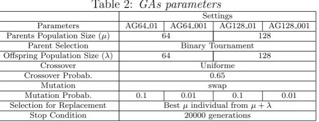
Previous adjustments on GA parameters are necessary to start the execution. In Table 2 are summarized those values. For evaluating the GAs, we have used the following func-tions: f15, f120, f25, f220,f35,f320 and f4. This set of test functions presents different

[image:7.595.142.459.352.473.2]

complexity degrees given their characteristics (unimodal, multimodal and deceptive) and their dimensions. Table 3 shows results obtained by a GA under different settings for each proposed test function.

Table 2: GAs parameters Settings

Parameters AG64 01 AG64 001 AG128 01 AG128 001 Parents Population Size (µ) 64 128

Parent Selection Binary Tournament Offspring Population Size (λ) 64 128

Crossover Uniforme

Crossover Probab. 0.65

Mutation swap

Mutation Probab. 0.1 0.01 0.1 0.01 Selection for Replacement Bestµindividual fromµ+λ

Stop Condition 20000 generations

Taking into account the quality of solutions, we can observe that all proposed alternative found the optimum for f15, f35, and f4 functions. Besides GA64 001 and GA128 001

reach the optimal solution for f120 and GA128 01 reaches it forf25 function.

When a population size is reduced and a mutation probability is low, the exploration of a search space can not be enough. A high mutation probability (0.1) allows to obtain the optimum the 100% of times for f15, f35 and f4. But if both parameters are reduced,

that is a population size of 64 and a mutation probability in 0.01, the percentage of hits is reduced to 13% for f35 and 53% for f4. When the population size and mutation

probability augment, we observe the best GA performance forf25,f35 andf4. A similar

behavior is observed for f35, f4 and f220, although in the last case the optimum is not

found.

Functions with 20 variables require a very rigorous adjustment of GA parameters; since they are functions which search space is 20-dimension. In this case, the best results are achieving when the mutation probability is 0.01. That means more exploration, during the search process, is necessary when the search space augments considerably.

(8)

[image:8.595.323.512.235.601.2]

For choices with a mutation probability of 0.001, the average number of generations to find the optimal solution is around 2900 generations when the population size is 64 and approximately 2300 when the population has 128 individuals. These values would be indicating a more appropriate stop condition in approximately 7000 generations. In this way, we establish an error margin since we are working with an average value. When we use a mutation probability of 0.01, the GA takes a 75% of total time to find the optimum which is equivalent to 12900 generations for populations with 64 individuals and 14000 generations when the population size is 128.

Table 3: GA Results GA64 01

Function %Hits AOT ATT AOI f15 100% 16.87 19.01 17732.13

f120 0% - 65.93

-f25 0% - 19.00

-f220 0% - 67.51

-f35 100% 17.13 19.40 17655.00

f320 0% - 70.07

-f4 100% 1.68 10.78 3110.70 GA64 001

f120 100% 20.47 63.80 6362.73

f25 0% - 18.49

-f220 0% - 64.74

-f35 13% 2.88 18.39 3102.25

f320 0% - 65.37

-f4 53% 1.08 9.83 2057.41 GA128 01

f120 0% - 133.28

-f25 3.3% 40.84 41.61 19675.00

f220 0% - 135.28

-f35 100% 35.84 40.49 18065.00

f320 0% - 136.83

-f4 100% 1.12 23.03 979.00 GA128 001

f120 100% 38.25 130.14 5818.30

f25 0% - 38.69

-f220 0% - 141.85

-f35 43% 2.57 38.35 1302.92

f320 0% - 132.40

-f4 60% 1.82 22.10 1637.22

Table 4: CHC Results CHC64 001

f120 100% 4.192 10.761 3822.00

f25 0% - 4.919

-f220 0% - 10.941

-f35 13% 0.586 5.216 2430.50

f320 0% - 11.953

-f4 53% 0.155 3.870 924.38 CHC64 002

f120 100% 2.182 11.341 1846.00

f25 7% 2.311 4.501 848.00

f220 0% - 11.383

-f35 23% 1.000 4.755 4299.43

f320 0% - 12.489

-f4 53% 0.078 3.499 2556.00 CHC128 001

f120 100% 7.474 22.668 4564.00

f25 0% - 11.729

-f220 0% - 23.133

-f35 33% 2.330 12.171 4000.40

f320 0% - 24.956

-f4 53% 1.295 9.220 2956.11 CHC128 002

f120 100% 4.980 25.062 2474.00

f25 0% - 10.954

-f220 0% - 24.149

-f35 27% 2.074 11.469 3687.25

f320 0% - 26.143

-f4 50% 2.394 8.693 5574.00

4.2 CHC Algorithm

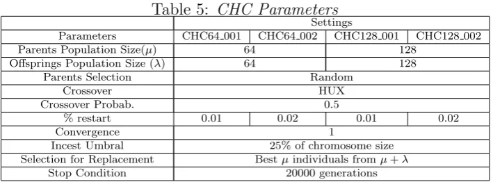
CHC requires to define a set of parametric values, for that we have reviewed some research works and we have did some test execution. In Table 5, we show the parametric values for CHC. Table 4 shows results obtained by CHC under different settings for each following test function: f15, f120,f25, f220, f35,f320, y f4.

Considering the quality of solutions, we observe all alternatives find the optimum in 4 (f15, f120,f35, andf4) of 7 tested functions. The exception is CHC64 002 which solves

optimally before 4 functions and f25. While if we analyze the percentage of hits we can

[image:8.595.81.274.237.599.2]

(9)

[image:9.595.121.476.107.238.2]

Table 5: CHC Parameters Settings

Parameters CHC64 001 CHC64 002 CHC128 001 CHC128 002 Parents Population Size(µ) 64 128

Offsprings Population Size (λ) 64 128

Parents Selection Random

Crossover HUX

Crossover Probab. 0.5

% restart 0.01 0.02 0.01 0.02

Convergence 1

Incest Umbral 25% of chromosome size Selection for Replacement Bestµindividuals fromµ+λ

Stop Condition 20000 generations

If we analyze globally the average time to find an optimum, we can observe that CHC does not take more than 3 seconds. Particularly, if the population size is 64, AOT is approximately 1,3 seconds (2000 generations) and if it is 128, AOT is around 2,8 seconds (3000 generations). That indicates the execution time increase is proportional to a population size increment. Besides CHC, under all parametric configurations, takes lesser than 21% of ATT to find an optimal solution. From these results we can define a new stop condition of 6000 generations when the population size is 64 and 7000 generations when the population has 128 individuals.

4.3 Scatter Search Algorthim

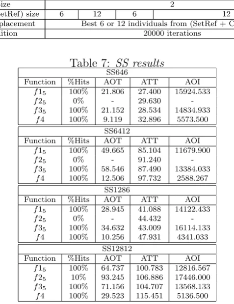
As for GAs and CHC, we have established different configurations for SS in Table 6. The test functions to evaluate SS are: f15, f25, f35, f4. We should reduced the test

set because when we used a search space 20-dimensional, the execution time was greater than 150 seconds and any optimum was found. That exceeds all execution times of GA and CHC algorithms. Table 7 resumes the obtained results from SS execution on test functions.

In this SS implementation, the SetRef is created in the following way: a fifty percent are formed by the best individuals of P, another fifty percent are formed by the most distant individuals from P. For that we use an Euclidean Distance.

In a first place, we analyze the quality of solutions. SS, under all configurations, finds the optimal solution for 3 (f15,f35 andf4) of 4 test functions with a 100% of hits. However

SS, under SS12812 configuration, obtains the optimum for f25 a 10% of times. A reason

for that is the greater diversity offered by this alternative, since P and SetRef sizes are the biggest ones. The high degree of epistasis which presents f2 requires many diverse solutions during the search.

(10)

[image:10.595.108.488.110.205.2]

Table 6: SS Parameters Settings

Parameters SS646 SS6412 SS1286 SS12812

Population SizeP 64 128

Improvement method each 50 iterations a gen value is changed with a proabability of 0.1

Crossover two points

Subset Size 2

Reference Set (SetRef) size 6 12 6 12 Selection for replacement Best 6 or 12 individuals from (SetRef + Children)

[image:10.595.178.417.168.478.2]

Stop Condition 20000 iterations

Table 7: SS results SS646

f25 0% - 29.630

-f35 100% 21.152 28.534 14834.933

f4 100% 9.119 32.896 5573.500 SS6412

f25 0% - 91.240

-f35 100% 58.546 87.490 13384.033

f4 100% 12.506 97.732 2588.267 SS1286

f25 0% - 44.432

-f35 100% 34.632 43.009 16114.133

f4 100% 10.256 47.931 4341.033 SS12812

f25 10% 93.245 106.886 17446.000

f35 100% 71.156 104.707 13568.133

f4 100% 29.523 115.451 5136.500

4.4 Comparison among GA, CHC and SS metaheuristics

In previous sections, we have analyzed each metaheuristic separately. Now, we make a comparison among them which objective is to detect what metaheuristic is preferable according to a given case.

Table 8 summarizes the best results obtained by each metahuristic for only test functions used for all them. From this Table and previous analysis, we can observe:

– Scatter Search is a metaheuristic very efficacious but not efficient. A reason is directly related with the SetRef building way; this considers the best solutions and the most different ones giving an adequate diversity, but it is a process with a high computational effort. This effort grows significantly when the chromosome size is augmented (more variables).

– GA and CHC present a similar performance for the unimodal function (f15); but

(11)

[image:11.595.212.385.107.320.2]

Table 8: GA, CHC and SS results %´exitos

GA CHC SS

f15 GA64 001 CHC64 001 SS646

100% 100% 100% f25 GA128 01 CHC64 02 SS646

3.3% 7% 10%

f35 GA128 001 CHC64 002 SS646

43% 23% 100%

f4 GA128 01 CHC64 002 SS646

100% 53% 100%

TPO

AG CHC SS

f15 AG64 001 CHC64 001 SS646

0.214 0.179 21.806 f25 AG128 01 CHC64 02 SS646

40.843 2.311 93.245 f35 AG128 001 CHC64 002 SS646

2.569 1.000 21.152 f4 AG128 01 CHC64 002 SS646 1.117 0.078 9.119

– If we consider the multimodal function (f3), CHC offers efficiency and GA offers provides efficacy.

– In general, for the deceptive function (f4), CHC is very efficient but GA is more efficacious.

5 CONCLUSIONS

In this paper, we have analyzed and compared three population-based metaheuristics: Genetic Algorithms, CHC algorithm and Scatter Search algorithm. Those metaheuristics are evaluated using a set of functions which represents many real problems.

Analyzing the results of experiments, we can infer that Scatter Search always achieves optimal values but the computational effort is very higher than GAs and CHC for all cases. While CHC and GAs can be used satisfactorily to solve problems which dimension can be incremented.

In the future we plan to make an genotypic analysis of population during the search process for GA, CHC and SS. Besides we want to study and compare another population-based metaheuristics.

REFERENCES

[1] T. Bck. Selective pressure in evolutionary algorithms: a characterization of selection mechanisms. InProceedings of the First IEEE Conference on Evolutionary Computation, pages 57–62, 1994.

[2] C. Blum and A. Roli. Metaheuristics in combinatorial optimization: Overview and conceptual comparison. Artificial Intelligence in Medicine, 35(3):268–308, 2003.

[3] A. Brindle.Genetic Algorithms for Function Optimization. Phd thesis, Department of Computer Science, University of Alberta, Edmonton, Alberta, 1981.

[4] L. J. Eshelman. The chc adaptive search algorithm: How to have safe search when engaging in nontraditional genetic recombination. InFoundations of Genetic Algorithms, pages 265– 283. Morgan Kaufmann, 1991.

[5] T. Feo and M. Resende. Greedy randomized adaptive search procedures.Journal of Global Optmization, (6):109–133, 1999.

(12)

[7] M. Gendreau. An introduction to tabu search. in f. glover, g. a.,handbook of metaheuristic. pages 37–54, 2003. [8] F. Glover. Heuristics for integer programming using surrogate constraints. Decision Sciences, 8:156–166, 1977. [9] F. Glover. Future paths for integer programming and links to articial intelligence.Computers and Operations Research,

(13):533–549, 1986.

[10] F. Glover. A template for scatter search and path relinking.selected papers from the third european conference on artificial evolution. In AE 97,London, UK, pages 13–54, 1998.

[11] D.E. Goldberg and K. Deb. A comparison of selection schemes used in genetic algorithms. InFoundations of Genetic Algorithms, pages 69–93, 1991.

[12] J. H. Holland.Adaptation in Natural and Artificial Systems. The MIT Press, Cambridge, Massachusetts, first edition, 1975.

[13] M Laguna and R. Mart. Experimental testing of advanced scatter search designs for global optimization of multimodal functions. Technical report, University of Colorado, Boulder, 2002.

[14] L. Li and S. Khuri. A Comparison of DNA Fragment Assembly Algorithms. InProceedings of the 2004 International Conference on Mathematics and Engineering Techniques in Medicine and Biological Sciences, pages 329–335, Las Vegas, 2004.

[15] G. Luque, E. Alba, and S. Khuri. Parallel Algorithms for Bioinformatics, chapter Chapter 16: Assembling DNA Fragments with a Distributed Genetic Algorithm. Wiley, New York, 2005.

[16] Dorigo M. Optimization, Learning and Natural Algorithms. PhD thesis, Politecnico di Milano, 1992.

[17] R. Mart, M. Laguna, and F. Glover. Principles of scatter search. European Journal of Operational Research 2006, 169:359–372, January 2004.

[18] Z. Michalewicz.Genetic Algorithms + Data Structures = Evolution Programs. Springer, third edition, 1999. [19] C. Notredame, L. Holm, and D.G. Higgins. COFFEE: an objective function for multiple sequence alignments.

Bioin-formatics, 14(5):407–422, 1998.

[20] R. Parsons, S. Forrest, and C. Burks. Genetic Algorithms, Operators, and DNA Fragment Assembly, 1993.

[21] C. Gelatt S. Kirkpatrick and M. Vecchi. Optimization by simulated annealing. Science, 220(4598):671–680, 1983. [22] Yuhui Shi. Particle swarm optimization.Electronic Data Systems, Inc. IEEE Neuronal Networks Society, 1994. [23] W.M. Spears and K.A. De Jong. On the virtues of parameterized uniform crossover. InProceedings of the Fourth

International Conference on Genetic Algorithms, pages 230–236, 1991.

[24] T. Sttzle. Local search algorithms for combinatorial problems analysis,algorithms and new applications. Technical report, Technical report, DISKI Dissertationen zur Knstliken Intelligenz, Sankt Augustin, Germany, 1999.

[25] G. Syswerda. Uniform crossover in genetic algorithms. Proceedings of the Third International Conference on Genetic Algorithms, San Mateo, California, pages 2–9, 1989.