VISION − Vienna survey in Orion

A&A 587, A153 (2016)

DOI:10.1051/0004-6361/201527160 c

ESO 2016

Astronomy

&

Astrophysics

VISION

−

_{Vienna survey in Orion}

I. VISTA Orion A Survey

Stefan Meingast

, João Alves

, Diego Mardones

, Paula Stella Teixeira

, Marco Lombardi

, Josefa Großschedl

,

Joana Ascenso

, Herve Bouy

, Jan Forbrich

, Alyssa Goodman

, Alvaro Hacar

, Birgit Hasenberger

,

Jouni Kainulainen

, Karolina Kubiak

, Charles Lada

, Elizabeth Lada

, André Moitinho

, Monika Petr-Gotzens

,

Lara Rodrigues

, and Carlos G. Román-Zúñiga

1 _{Department of Astrophysics, University of Vienna, Türkenschanzstrasse 17, 1180 Wien, Austria} e-mail:stefan.meingast@univie.ac.at

2 _{Departamento de Astronomía, Universidad de Chile, Casilla 36-D, Santiago, Chile} 3 _{University of Milan, Department of Physics, via Celoria 16, 20133 Milan, Italy}

4 _{CENTRA, Instituto Superior Tecnico, Universidade de Lisboa, Av. Rovisco Pais 1, 1049-001 Lisbon, Portugal} 5 _{Universidade do Porto, Departamento de Engenharia Física da Faculdade de Engenharia, Rua Dr. Roberto Frias, s/n,}

4200-465 Porto, Portugal

6 _{Centro de Astrobiología, INTA-CSIC, Depto Astrofísica, PO Box 78, 28691 Villanueva de la Cañada, Madrid, Spain} 7 _{Harvard-Smithsonian Center for Astrophysics, 60 Garden Street, Cambridge, MA 02138, USA}

8 _{Max-Planck-Institute for Astronomy, Königstuhl 17, 69117 Heidelberg, Germany} 9 _{Astronomy Department, University of Florida, Gainesville, FL 32611, USA}

10 _{SIM/CENTRA, Faculdade de Ciencias de Universidade de Lisboa, Ed. C8, Campo Grande, 1749-016 Lisboa, Portugal} 11 _{European Southern Observatory, Karl-Schwarzschild-Str. 2, 85748 Garching, Germany}

12 _{Instituto de Astronomía, UNAM, Ensenada, CP 22860, Baja California, Mexico}

Received 10 August 2015/Accepted 1 December 2015

ABSTRACT

Context.Orion A hosts the nearest massive star factory, thus offering a unique opportunity to resolve the processes connected with the formation of both low- and high-mass stars. Here we present the most detailed and sensitive near-infrared (NIR) observations of the entire molecular cloud to date.

Aims.With the unique combination of high image quality, survey coverage, and sensitivity, our NIR survey of Orion A aims at establishing a solid empirical foundation for further studies of this important cloud. In this first paper we present the observations, data reduction, and source catalog generation. To demonstrate the data quality, we present a first application of our catalog to estimate the number of stars currently forming inside Orion A and to verify the existence of a more evolved young foreground population.

Methods.We used the European Southern Observatory’s (ESO) Visible and Infrared Survey Telescope for Astronomy (VISTA) to survey the entire Orion A molecular cloud in the NIRJ,H, andKSbands, covering a total of∼18.3 deg2_{. We implemented all data} reduction recipes independently of the ESO pipeline. Estimates of the young populations toward Orion A are derived via theKS-band luminosity function.

Results.Our catalog (799 995 sources) increases the source counts compared to the Two Micron All Sky Survey by about an order of magnitude. The 90% completeness limits are 20.4, 19.9, and 19.0 mag inJ,H, and KS, respectively. The reduced images have 20% better resolution on average compared to pipeline products. We find between 2300 and 3000 embedded objects in Orion A and confirm that there is an extended foreground population above the Galactic field, in agreement with previous work.

Conclusions.The Orion A VISTA catalog represents the most detailed NIR view of the nearest massive star-forming region and provides a fundamental basis for future studies of star formation processes toward Orion.

Key words.techniques: image processing – methods: data analysis – stars: formation – stars: pre-main sequence

1. Introduction

One of the major obstacles since the beginning of star forma-tion studies in the late 1940s is that stars are embedded in molecular gas and dust during their formation and early evo-lution, inaccessible to optical imaging devices. The deployment of infrared imaging cameras on optical- and infrared-optimized ? _{Based on observations made with ESO Telescopes at the La Silla}

Paranal Observatory under program ID 090.C-0797(A). ??

Image data and full Table B.1 are only available at the CDS via anonymous ftp tocdsarc.u-strasbg.fr(130.79.128.5) or via

http://cdsarc.u-strasbg.fr/viz-bin/qcat?J/A+A/587/A153

OMC 2

OMC 3

L1641

NGC 1977

L1647

V380/HH1-2

L1641-S

L1641-C

L1641-N

NGC 1980

NGC 1981

M42

Saiph

214

212

210

208

-18

-19

-20

Galactic Longitude (°)

Galactic Latitude (°)

10

10

10

10

10

10

# References

Fig. 1.Composite of optical data (image courtesy of Roberto Bernal Andreo; deepskycolors.com) overlayed withPlanck-Herschelcolumn density measurements of Orion A in green. Approximate positions of noteworthy objects and regions are marked and labeled.On top, a histogram (note the logarithmic scaling) shows the number of references for all objects in the SIMBAD database at a given galactic longitude with a 3 arcmin bin size. We see an extreme gradient in attention paid to the various portions of the cloud, with the peak coinciding with M42 and the ONC. Prominent objects (e.g., the V380/HH 1−2 region) produce a local spike in the reference histogram whereas the bulk of the molecular cloud has been studied in comparatively few articles. The coordinates of L1647 in the SIMBAD database (l=212.13,b=−19.2) do not match the original publication (l=214.09,b=−20.04).

deployment of active- and adaptive-optics systems on 8−10 m class telescopes, combined with advanced instrumentation, has allowed ground-based NIR observations to match the supreme sensitivity of space-borne observatories but reaching higher spa-tial resolutions thanks to the larger apertures, which is critical to star formation research.

Over the past 25 years, systematic NIR imaging surveys of molecular clouds, in particular of the Orion giant molecular clouds, have revealed much of what we currently know about the numbers and distributions of young stars in star-forming regions. For example, the early foundational NIR surveys (e.g., Lada et al. 1991;Strom et al. 1993;Chen & Tokunaga 1994;Hodapp 1994;Ali & Depoy 1995;Phelps & Lada 1997;Carpenter 2000; Carpenter et al. 2000;Davis et al. 2009) revealed the importance of embedded clusters in the star-forming process. By combining information on the distribution of young stars with surveys of the distribution and properties of molecular gas, important in-sight into how nature transforms gas into stars have been gained (e.g.,Lada 1992;Carpenter et al. 1995;Lada et al. 1997,2008; Megeath & Wilson 1997;Carpenter et al. 2000;Teixeira et al. 2006;Román-Zúñiga et al. 2008;Evans et al. 2009;Gutermuth et al. 2009,2011).

In the Orion star-forming complex, one finds a few of the best-studied testbeds for star formation theories, such as the embedded clusters NGC 2024, NGC 2068, and NGC 2071, as well as the optically visible young clusters λ,σOri,ιOri, and NGC 1981. However, none of these regions have drawn nearly as much attention as the famous Orion nebula cluster (ONC), embedded in the Orion A molecular cloud. The ONC itself is the closest massive star factory and therefore a prime laboratory

for addressing many open questions of current star formation re-search. Many fundamental quantities regarding the formation of stars have been tested against this benchmark cluster, but orders of magnitude fewer studies have been published about objects in other parts of Orion A, and even fewer have addressed the molecular cloud as a whole, creating a biased view of the re-gion. To help visualize this bias, we show in Fig.1 a compos-ite of an optical image overlaid on theHerschel-Planckcolumn density map fromLombardi et al.(2014). Here we marked sev-eral objects and star-forming regions throughout Orion A, which is mentioned later in this paper. On top of the image we plot a histogram of the number of articles referenced in the SIMBAD (Wenger et al. 2000) database1_{for all objects at a given longitude} slice in bins of 3 arcmin.

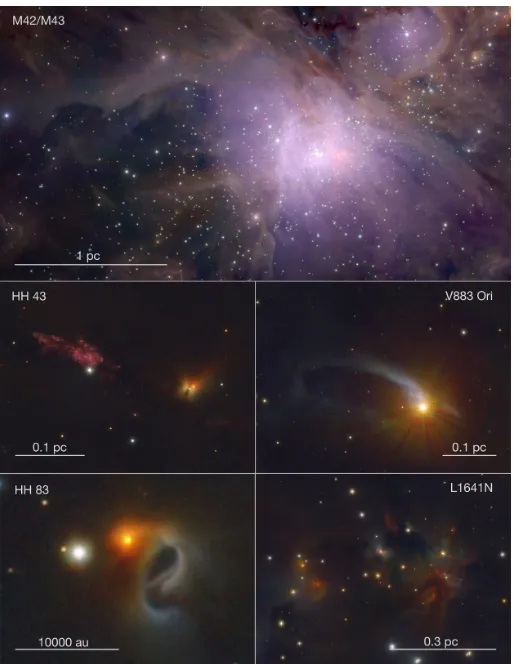
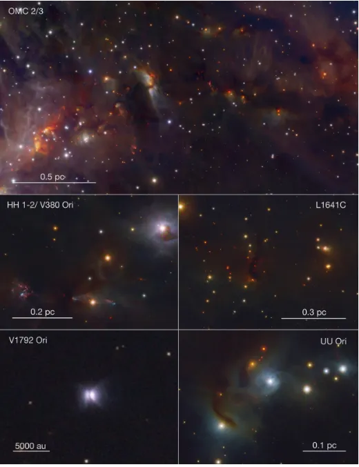
While the ONC and its surroundings are subject to various studies in thousands of articles, objects in the eastern region of the cloud (in galactic frame2_{) receive considerably less attention} with a few tens of published studies. We note that the SIMBAD database is not complete, nonetheless these numbers are a good indicator of the bias in the astronomical community for some re-gions of Orion A. Figures2and3show examples of prominent objects observed in our survey of Orion A. Together, these ob-jects alone have more than 5000 bibliographic references listed in the SIMBAD database.

While previous NIR surveys of Orion A have given us im-portant insights, they are limited in their depth and ensitivity 1 _{The references were extracted from the SIMBAD database on 2015} May 10.

Table 1.On-sky coverage and relative gain in source counts for selected NIR surveys toward Orion A.

Reference Coveragea _Gainb _Bands

(arcmin2₎

Strom et al.(1993) 2772 ∼4−6c _JHK

Ali & Depoy(1995) 1472 4 K

Carpenter(2000)d _{65 857 9.3 JHKS}

Lawrence et al.(2007)e _{∼26 500 1.4 ZY JHKS}

Robberto et al.(2010) 1200 1.4 JHKS

This work 65 857 JHKS

Notes.Our survey improves both coverage and sensitivity when com-pared to the literature.(a)_{Refers to the common on-sky area of the given} survey with our VISTA coverage.(b)_{Approximate gain in source counts} when restricted to the same on-sky coverage.(c)_{Estimate based on} com-pleteness limits since no source catalog is available.(d)_{Study based on} the second incremental 2MASS data release. Source counts in this ta-ble were taken from the final 2MASS all-sky data release.(e)_{Data from} UKIDSS DR10. Because of the many spurious detections of nebulos-ity in the UKIDSS survey, we estimated the gain in source counts by selecting a “clean” subregion.

and/or only cover a fraction of the entire molecular cloud. As a fundamental step toward a complete picture of the star for-mation processes in Orion A, we present the most sensitive NIR survey of an entire massive star-forming molecular cloud yet. Table1lists NIR surveys throughout the past two decades. Compared to the ONC surveys from the 1990s, our survey is about four times more sensitive (in terms of source counts) and covers a∼50 times larger area at the same time. Moreover, we also increase source counts by about 40% compared to the more recent dedicated NIR survey of the ONC by Robberto et al. (2010). Compared to the Two Micron All Sky Survey (2MASS, Skrutskie et al. 2006), which obviously has a greater coverage, we gain almost a factor of 10 in sensitivity. For completeness we mention here that a similar survey has been conducted of the Orion B molecular cloud. These results are presented inSpezzi et al.(2015).

The target of our survey, the Orion A giant molecular cloud, extends for about 8 deg (∼60 pc) and contains several well-studied objects and an extensive literature: we refer the reader to the review papers of Bally (2008), Briceno (2008),O’Dell et al.(2008),Allen & Davis(2008),Alcalá et al.(2008),Muench et al.(2008), andPeterson & Megeath(2008). Here we only list a selection of the many results for this important region, includ-ing studies of the ONC (Hillenbrand & Hartmann 1998; Lada et al. 2000;Muench et al. 2002;Da Rio et al. 2012), Herbig-Haro objects (HH; for a historic overview, see, e.g., Reipurth & Heathcote 1997), such as HH 1-2 (see, e.g.,Herbig & Jones 1983;Lada 1985;Fischer et al. 2010) and HH 34 (e.g.,Reipurth et al. 2002), and variable FU Ori type pre-main-sequence stars such as V883 (e.g.,Strom & Strom 1993;Pillitteri et al. 2013). Along the “spine” of Orion A, there are also multiple notewor-thy minor star-forming regions, such as L1641-N (e.g.,Gâlfalk & Olofsson 2008;Nakamura et al. 2012), which are themselves, however, much less prominent than the Orion nebula and its surroundings.

Studies referring to the entire cloud are rare.Megeath et al. (2012) present a Spitzer-based catalog of young stellar ob-jects (YSO) for both Orion A and Orion B. They identify 2446 pre-main-sequence stars with disks and 329 protostars in Orion A. Pillitteri et al. (2013) present an XMM-Newton sur-vey of L1641 where they investigate clustering properties of

Class II and Class III YSOs. They find an unequal spatial distri-bution in L1641, which suggests multiple star formation events along the line of sight, in agreement with the interpretation of Alves & Bouy(2012) andBouy et al.(2014), and migration of older stars. More recently,Lombardi et al.(2014) have used a 2MASS dust extinction map (Lombardi et al. 2011), along with Planck dust emission measurements, to calibrateHerscheldata and construct higher angular-resolution and high dynamic range column-density and effective dust-temperature maps. Stutz & Kainulainen(2015) investigate variations in the probability dis-tribution functions of individual star-forming clouds in Orion A and suggest a connection between the shape of the distribution functions and the evolutionary state of the gas.

Regarding the overall evolution of the Orion star-forming re-gion and followingBlaauw(1964),Gomez & Lada(1998) spec-ulated on the presence of multiple overlapping populations in the direction of the ONC with a possible triggered star forma-tion scenario. As also menforma-tioned byBally(2008), recent stud-ies by Alves & Bouy (2012) and Bouy et al. (2014) reveal a slightly older foreground population associated with NGC 1980 with distance and age estimates of ∼380 pc and 5−10 Myr, respectively. They find 2123 potential members for this fore-ground population, which, however, is an incomplete estimate, because they did not cover the entire Orion A molecular cloud owing to lack of data in the eastern regions. Based on a shift in X-ray luminosity functions across Orion A,Pillitteri et al. (2013) also find evidence of a more evolved foreground popu-lation near NGC 1980 at a distance of 300−320 pc. Proposing an alternative view,Da Rio et al.(2015) find that sources near NGC 1980 do not have significantly different kinematic proper-ties from the embedded population, concluding that NGC 1980 is part of Orion A’s star formation history and is currently emerg-ing from the cloud.

Early distance estimates from Trumpler (1931) placed the ONC at 540 pc. Subsequent studies find distances of 480±80 pc (Genzel et al. 1981), 437±19 pc (Hirota et al. 2007), 389+₋24₂₁pc (Sandstrom et al. 2007), 440±34 pc (392±32 pc with a different subset of target stars,Jeffries 2007), and 371±10 pc (Lombardi et al. 2011). Based on optical photometry and aPlanck-based dust screen model, Schlafly et al. (2014) find a distance of 420±42 pc toward the ONC, while the eastern edge of Orion A appears to be 70 pc more distant. For the remainder of this paper, we adopt the distance of 414±7 pc fromMenten et al.(2007).

The VISION (VIenna Survey In OrioN) data presented in this paper (Orion A source catalog and three-color image mo-saic) are made available to the community via CDS. In future publications the survey data will allow us and the community to refine, extend, and characterize several critical properties of Orion A as a whole. This includes characterizing individual YSOs with the improved resolution and sensitivity, searching for HH objects and jets in a uniform manner, characterizing YSO clustering properties, determining IMFs down to the brown dwarf regime, and describing the gas mass distribution with re-spect to YSO positions.

Control field

VISTA survey

240 230 220 210

-10

-15

-20

Galactic Longitude (°)

Galactic Latitude (°)

S1 S2 S3 S4 S5 S6

N1 N2 N3 N4 N5

216 214 212 210 208 206

-18

-19

-20

-21

Galactic Longitude (°)

0.0 0.5 1.0 1.5 2.0

AK

(m

ag

)

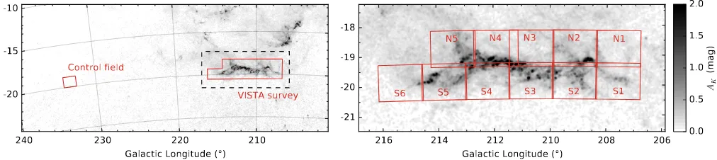
Fig. 4.VISTA survey coverage. Thelefthand side plotshows the wide-field extinction map fromLombardi et al.(2011) with both the control field and Orion A coverage marked as red boxes. Therighthand side figureshows a close-up of Orion A with the individual tiles labeled. The cutout region of this figure is marked with a black dashed box in theleft plot.

appearance and new candidate galaxy clusters. In Sect. 5 we present first results obtained from this new database, where we derive an estimate for the YSO population in Orion A and in-vestigate the foreground populations. Section6contains a brief summary, and AppendicesAandBcontain additional informa-tion on the quality of the data products and supplementary data tables, respectively.

2. Observations

2.1. Instrumentation

The observations of the Orion A molecular cloud have been carried out with the Visible and Infrared Survey Telescope for Astronomy (VISTA, Emerson et al. 2006), a 4 m class tele-scope that is operated by the European Southern Observatory (ESO) as part of its Cerro Paranal facilities. A single instru-ment, the VISTA Infrared Camera (VIRCAM, Dalton et al. 2006), is attached to the telescope’s Cassegrain mount, which offers a range of broadband and narrowband filters in the NIR covering a wavelength range from about 0.85 µm to 2.4 µm. VIRCAM features a set of sixteen 2k ×2k Raytheon VIRGO detectors arranged in a sparse 4×4 pattern. Each detector cov-ers about 11.6×11.6 arcmin on sky with gaps of 10.4 arcmin and 4.9 arcmin between them in the instrument’s X/Y setup, re-spectively. Working at a mean pixel scale of 0.339 arcsec/pix in both axes, the instrument field of view in the telescope’s beam is 1.292×1.017 deg.

The detectors offer a quantum efficiency above 90% across the J,H,andKSbands but suffer from significant cosmetic defi-ciencies (e.g., bad pixel rows and columns, as well as bad read-out channels) and nonlinearity effects, which need to be taken care of during data calibration. The gaps between the individ-ual detectors make it necessary to observe multiple overlapping fields for a contiguous coverage. This is achieved by a six-step offset pattern that can be executed in several ways. As a conse-quence of this observing strategy, the effective coverage (hence exposure time) over a single field varies with position. The stan-dard offset pattern offers a coverage of as little as just one frame on the edge of the field, two frames for most of the area and up to six overlapping exposures for only a tiny portion of the final frame. As is usual for NIR observations, a dither or jitter3_pattern is usually executed at each offset position to mitigate saturation effects and to increase the total frame coverage to facilitate bad pixel rejection during co-addition.

3 _{Here we use the term dither for user-defined offset positions, whereas} jitter refers to random telescope positioning.

For the rest of this paper, we use VISTA terminology to describe the telescope’s data products and its parameters: a simultaneous integration from all sixteen detectors is called a “pawprint”, and a fully sampled image resulting from the co-added frames of the six-step offset pattern is called a “tile”. The integration time for a single readout from all detectors is referred to as DIT (detector integration time), whereas multiples of these single integrations can be stacked internally before readout. The number of integrations in such a stack is referred to as NDIT.

2.2. Survey design and strategy

The Orion A molecular cloud is centered at approximatelyl = 210◦_{,b = −19}◦ _{and extends for about eight degrees, which is} well aligned with the Galactic plane. The spine of the cloud (i.e., regions with high extinction) is very narrow with only about 0.3 deg at its widest point. However, shallower extinc-tion levels are observed much more widely, which did not allow us to cover the entire cloud with only one series of pointings along the molecular ridge. Therefore we designed the survey to feature 11 individual pointings with two parallel sequences of tiles aligned with its spine. For each tile we also included over-laps with its neighboring field to ensure a contiguous coverage. Figure4 shows the final tile coverage on top of the extinction map fromLombardi et al.(2011). Also shown are our designa-tions for each tile labeled from N1, ..., N5, S1, ..., S6 indicating row (north/south) and column position (west to east). An obser-vation of a tile in one of the three filters defined an obserobser-vation block (OB). All 11 tiles were observed inJ,H,andKS, where all except the tiles N2 and S2 were executed with a standard jit-ter patjit-tern with a maximum random throw within a 25 arcsec wide box centered on the initially acquired position. The N2 and S2 tiles include the ONC and therefore a large amount of ex-tended emission. These positions were observed with a separate sky offset field centered atl=209.272◦_,b=−21.913◦_{. Because} the sky offset field had to be observed in addition to the science fields, the total duration of these sequences was greater than the maximum allowed OB length of one hour in theHandKSbands. Therefore each of these four OBs was executed twice. Starting in October 2012 and spreading out over about six months until early March 2013, a total of 37 individual OBs were executed to complete the observations of Orion A.

Table 2.Observing dates and basic parameters for the Orion A VISTA survey.

Tile ID filter Start time DIT NDIT NJitter Airmass range Image qualitya _{90% Completeness}b

UT (s) (#) (#) (arcsec) (mag)

S1 J 2012/10/02 08:38:24 5 8 3 1.074−1.088 0.78−0.92 20.47

S1 H 2013/02/27 02:09:44 2 27 5 1.308−1.657 0.68−0.83 20.06

S1 KS 2013/01/20 00:23:40 2 20 5 1.110−1.197 0.63−1.02 18.91

S2 J 2012/12/25 05:20:26 5 9 6 1.122−1.328 0.75−0.86 20.08

S2 (a) H 2013/02/08 01:17:15 2 17 5 1.058−1.136 0.72−0.89 19.58

S2 (b) H 2013/02/17 01:24:44 2 17 5 1.089−1.245 0.75−0.89 19.58

S2 (a)c _{KS 2013/01/25 00:35:11 2 15 5 1.060−1.125 0.87−1.06 18.85}

S2 (b) KS 2012/10/04 08:07:02 2 15 5 1.058−1.112 0.62−0.75 18.85

S3 J 2012/10/05 08:39:35 5 8 3 1.054−1.064 0.61−0.69 20.87

S3 H 2013/03/02 01:12:20 2 27 5 1.137−1.319 0.70−0.84 20.01

S3 KS 2013/01/30 00:33:06 2 20 5 1.054−1.093 0.67−0.81 19.08

S4 J 2012/11/13 08:09:40 5 8 3 1.103−1.143 0.70−0.92 20.48

S4 H 2013/03/01 02:18:03 2 27 5 1.304−1.665 0.65−0.91 20.27

S4 KS 2013/02/09 01:30:51 2 20 5 1.048−1.093 0.63−0.88 19.13

S5 J 2013/02/24 02:53:52 5 8 3 1.352−1.461 0.66−0.92 20.41

S5 H 2013/03/06 00:30:46 2 27 5 1.072−1.189 0.62−0.82 20.25

S5 KS 2013/02/16 01:45:14 2 20 5 1.076−1.162 0.81−1.04 18.97

S6 J 2013/02/24 03:35:28 5 8 3 1.573−1.750 0.76−0.96 20.23

S6 H 2013/03/09 00:22:19 2 27 5 1.066−1.182 0.80−1.09 19.69

S6 KS 2013/01/31 00:30:20 2 20 5 1.037−1.080 0.72−1.00 18.95

N1 J 2012/11/13 07:48:48 5 8 3 1.108−1.141 0.72−0.86 20.55

N1 H 2013/02/27 00:09:19 2 27 5 1.072−1.135 0.65−0.86 20.26

N1 KS 2013/01/27 00:38:09 2 20 5 1.077−1.122 0.69−0.84 19.17

N2 J 2013/02/25 02:23:36 5 9 6 1.298−1.753 0.78−0.97 20.14

N2 (a) H 2013/02/28 01:07:48 2 17 5 1.125−1.337 0.66−0.84 19.69

N2 (b) H 2013/03/01 00:56:10 2 17 5 1.112−1.306 0.64−0.78 19.69

N2 (a) KS 2013/01/28 00:40:27 2 15 5 1.060−1.107 0.81−0.93 18.86

N2 (b) KS 2013/01/29 00:45:10 2 15 5 1.059−1.096 0.84−0.98 18.86

N3 J 2012/11/04 08:10:11 5 8 3 1.070−1.092 0.58−0.78 20.84

N3 H 2013/03/03 01:58:40 2 27 5 1.270−1.588 0.70−0.89 20.16

N3 KS 2013/02/01 00:31:35 2 20 5 1.056−1.093 0.66−0.88 19.20

N4 J 2012/11/15 07:41:11 5 8 3 1.075−1.103 0.64−1.03 20.70

N4 H 2013/03/03 23:58:43 2 27 5 1.050−1.111 0.60−0.79 20.16

N4 KS 2013/02/15 00:19:06 2 20 5 1.045−1.050 0.80−1.18 18.83

N5 J 2013/02/24 03:14:42 5 8 3 1.452−1.590 0.78−0.93 20.40

N5 H 2013/03/07 01:16:29 2 27 5 1.158−1.369 0.62−0.84 20.18

N5 KS 2013/02/16 00:33:10 2 20 5 1.038−1.073 0.88−1.02 18.92

CF J 2013/01/02 07:40:14 5 8 3 1.484−1.624 0.63−0.76 20.67

CF H 2013/02/15 03:48:50 2 27 5 1.216−1.489 0.65−0.95 19.78

CF KS 2013/02/18 04:08:35 2 20 5 1.339−1.609 0.67−0.87 18.99

Notes.(a)_{The image quality refers to measured FWHM estimates of point-like sources, which varies across each tile because of camera distortion} and variable observing conditions.(b)_{Completeness estimates are derived from the full combined Orion A mosaics and are calculated on the basis} of artificial star tests. Details on the method are described inA.1.(c)_{Rejected in co-addition due to large differences in image quality with respect} to Tile S2 (b).)

was chosen to be only 2 s owing to saturation issues and was compensated by increasing numbers of NDIT ranging from 15 to 27 for these bands. In theJband we reached a more efficient duty cycle with larger DITs since saturation is less critical at this wavelength. The number of jitter positions at each of the six tele-scope offsets to form a tile was chosen to be a minimum of 3three for theJband to allow for reliable bad pixel rejection. For theH andKSbands, we observed five jittered positions for each paw-print. The total on-source exposure time is given by the product of the minimum exposure time (DIT×NDIT) and the number of observations taken at this position determined by Njitter and the six-step offset pattern. For the large majority of sources in a tile, this is given by DIT×NDIT×Njitter×2.

In addition to the science and control fields, calibration frames were also needed to process the raw files into usable data products. Dark frames, sky flat fields for each band, and dome

flats to measure detector nonlinearity were provided as part of ESO’s standard calibration plan for VIRCAM.

3. Data processing

30 20 10 0 10 20 30 ∆X (arcmin)

40 30 20 10 0 10 20 30 40

∆

Y (

ar

cm

in)

Our reduction

30 20 10 0 10 20 30

∆X (arcmin)

CASU reduction

0.72 0.76 0.80 0.84 0.88 0.92 0.96 1.00PSF FWHM (arcsec)

30 20 10 0 10 20 30

∆X (arcmin)

40 30 20 10 0

10 20 30 40

∆

Y (

ar

cm

in)

Resolution gain

16.8 17.6 18.4 19.2 20.0 20.8 21.6 22.4Difference (%)

Fig. 5.FWHM maps for both our reduction and the standard CASU pipeline of tile S1 inHband. Clearly a significant gain in image quality is achieved in our reduction.

VISTA Orion A survey, we decided to implement all key data reduction procedures ourselves. Details on the methods, includ-ing a mathematical description of the CASU pipeline modules, can be found in the VISTA data reduction library design and as-sociated documents4_.

3.1. Motivation

Below we list the specific points that motivated us to develop our own customized reduction pipeline for the Orion A VISTA data.

– Owing to the observing strategy with VIRCAM, sources are sampled several times not only at different detector positions but also by different detectors. To optimally co-add all re-duced paw prints, each input image needs to be resampled and aligned with a chosen final tile projection. The CASU pipeline uses a radial distortion model, together with fast bi-linear interpolation, to remap the images for the final tiling step. Bilinear interpolation, however, has several drawbacks. Primarily it can introduce zero-point offsets and a signifi-cant dispersion in the measured fluxes. Typically a Moiré pattern is also seen on the background noise, and addition-ally it “smudges” the images, leading to lower output res-olution (seeBertin 2010for details and examples). To test for the absolute gain in resolution over the bilinear resam-pling kernel, full width half maximum (FWHM) maps for each observed tile were calculated with PSFex (Bertin 2011). Figure 5 shows a FWHM map for the tile S1 in H band for both the CASU and our reduction, as well as the gain in resolution. We typically achieve 20% higher resolution, i.e. a 20% smaller FWHM, by simply using more suitable resampling kernels5 (for an interesting in-depth discussion 4 _{Accessible through http://casu.ast.cam.ac.uk, Lewis et al.} 2010.

5 _{We observed a dependency of the resolution gain on observing} con-ditions. We get only 10−15% for bad seeing conditions (>1 arcsec) and up to almost 30% for excellent conditions (∼0.6 arcsec)

of the importance of resampling methods, see, e.g., Lang 2014). We find that our resampling method recovers the image quality of the pawprint level for the combined tiles, which is not the case for the CASU reduction.

– The CASU pipeline only produces source catalogs for indi-vidual tiles. As can be seen in Fig.4, it would be beneficial to co-add all input tiles to increase the effective coverage on the tile’s edges and run the source extraction on the entire survey region. The spatially correlated noise (which is not traced by weight maps) and the necessity of yet another resampling pass make this step highly undesirable for the CASU tiles.

– Even with such short integration times as in our survey, stars brighter than∼12th magnitude inJ(11.5 and 11 mag inH andKS, respectively) show saturation and residual nonlinear-ity effects when compared to the 2MASS catalog. Replacing these measurements with reliable photometry from 2MASS requires that both catalogs are calibrated toward the same photometric system. As already demonstrated byGonzalez et al.(2011), among others, this is not the case, and a com-parison with 2MASS requires the recalibration of the pho-tometric zero point. Reliable color transformations can be found inSoto et al.(2013). We also tested this by produc-ing magnitudes from the CASU tile catalogs via

mi,j=−2.5 log

Fi,j

tj

!

−apcor_j+ZPj (1)

wheremi,j are the calculated magnitudes for theith source

measured on the jth tile, Fi,j the flux measurements given

in the CASU tile catalogs, tj the exposure times, apcorj

the aperture corrections, and ZPj the zero points as given

Fig. 6. Difference in the photometry between the CASU default re-duction and the 2MASS catalog. The blue, green, and red data points show theJ,H, andKSbands, respectively. The color shading represents source density in a 0.2×0.05 box in the given parameter space and the gray solid line a running median along the abscissa with a box width of 0.5 mag. Several processing steps contribute to the apparent offsets, which are all avoided in our data reduction.

A systematic offset is visible with values around 0.1 mag in Hand 0.12 mag inKS.

– For the zero-point calculation of each observed field, the CASU pipeline applies a galactic extinction correction to all photometric measurements. To this end the pipeline uses the Schlegel et al.(1998) all-sky extinction maps (with a resolu-tion of a few arc-minutes), together with the correcresolu-tion from Bonifacio et al.(2000). For each source, a bilinear interpola-tion yields the extincinterpola-tion correcinterpola-tion factor for the zero point. This will also add systematic offsets with respect to photo-metric data for which no such correction was applied. More critically, for surveys covering multiple fields with variable extinction, systematic offsets are expected between the tiles. For studies concerned with the intrinsic color of stars (e.g., extinction mapping), however, it is critical not to be biased in any way by such systematic offsets.

– The CASU pipeline by default stacks all frames of an entire set to build a single background model for one tile. This only works well if spatial sky variations across the detector array are constant for the entire duration of the observations. In the NIR this typically applies for small sets of data with rel-atively short total exposure times, such as for the VISTA sur-vey products (e.g., VVV,Minniti et al. 2010). However, since our OBs were at the limit of the maximum allowed execution time of 1 h, significant changes in atmospheric conditions are expected for nonphotometric nights. This can lead to resid-ual gradients across single detector frames, which can result in cosmetically imperfect reductions and difficult sky level estimates. This is especially the case for fields with separate offset sky positions with large gaps in the sky sampling.

– In total there are two interpolation steps employed by the CASU pipeline. The first generates stacks for each jitter sequence, and the second is used during the tiling proce-dure to correct for astrometric and photometric distortions (the latter to account for variable on-sky pixel size due to field distortion). Both of these steps use bilinear interpo-lation, which can introduce spatially correlated noise. The

30 15 0 15 30

∆X (arcmin)

40 20 0 20 40

∆

Y (

ar

cm

in)

Our reduction

30 15 0 15 30

∆X (arcmin)

40 20 0 20 40 CASU 0.8 0.9Normalized background RMS1.0 1.1 1.2

Fig. 7. Noise rms maps of the CF in KS for our reduction and the CASU pipeline. The bilinear interpolation and the radial distortion model clearly leave spatially correlated noise in the tiled images. On the other hand, the variance in our reduction is only dominated by de-tector coverage and intrinsic dede-tector characteristics. No sources were masked prior to noise calculations.

difference between the original bilinear interpolation and our data product, for which we use higher order resampling ker-nels, is illustrated in Fig.7, where the background rms maps of the CF in theKS band are shown. The radial distortion model, together with the fast interpolation, clearly leaves its mark. These rms maps were generated with SExtractor (Bertin & Arnouts 1996) and represent smoothed-noise rms models with a background mesh size of 64 pixels. For reli-able source detection, however, one has to keep track of the variable noise throughout an image. As a consequence this makes it difficult to reliably run external source detection packages on the output CASU tiles in cases the pipeline does not work satisfactorily, as in regions with extended emission such as the ONC.

From all these points, only the photometric offset relative to the 2MASS system can be corrected for via color transformations. Bias-free photometry and high resolution are both critical for all further studies with the Orion A VISTA data. Therefore we have written a semi-automatic data-reduction package that is com-pletely independent of the CASU pipeline. All functionalities of this package will be offered in open-source Python code in a fu-ture paper. The implemented reduction steps are discussed in de-tail during the following sections. In summary, the following ca-pabilities have been implemented specifically for the VIRCAM reduction package:

– calculation of all required master calibration frames and pa-rameters: bad pixel masks (BPM), dark frames, flat fields, and nonlinearity coefficients;

– basic image calibration: nonlinearity correction, removal of the dark current, and first-order gain harmonization with the master flat;

– accurate weight map generation for co-addition and source detection;

– static and dynamic background modeling;

– removal of cosmetic deficiencies (bad pixel masking, global background harmonization, etc.);

– source detection, astrometric calibration, and co-addition via external packages;

– robust aperture photometry using variable aperture corrections;

– photometric calibration based on the 2MASS reference cat-alog (Vega magnitude system).

Many of the techniques are similar to the methods used in the CASU pipeline. However, the problems listed above are care-fully avoided. All sequential data reduction procedures are de-scribed in the following sections.

3.2. Master calibration frames

The basic image reduction steps include the generation of all required calibration frames and parameters and their application to the raw science data to remove the instrumental signature from VIRCAM.

3.2.1. Bad pixel masking

Before any other calibration step can be performed, a BPM is required to avoid introducing systematic offsets in, for in-stance, dark current calculations or linearity estimations. This step, however, has to be independent of any further calibration steps. Therefore we used a set of dome flats with constant ex-posure times that are first stacked at the detector level. The me-dian of each detector served as a preliminary master flat and was then used to normalize each input image. Good pixels in each recorded flat field would then theoretically contain only values around unity due to the constant exposure time. Then, all pix-els that deviated by more than 4% with respect to the expected unity value were marked. Finally, if a single pixel was marked in this way in more than 20% of all images in the sequence, it was propagated as a bad pixel to the final master BPM. Typical bad pixel-count fractions were found between 0.1% and 0.2% for the best detectors and around 2% for the worst.

3.2.2. Nonlinearity correction

To correct for detector nonlinearities, we used the same method as for the CASU pipeline. For details on this method, the reader is referred to the VISTA data reduction library design docu-ment6_{. In principle a set of dome flat fields with increasing} expo-sure time was first masked, i.e. with the BPM and pixels above the saturation level, and corrected for dark current with the ac-companying dark frames. Then the flux was determined for the detector as the mode of each masked frame. The increasing ex-posure time should then provide a constant slope in the flux vs. exposure time relation for a completely linear detector with a given constant zero point (in double-correlated read mode used for our observations this offset should be close to 0). A least-squares fit to these data using a function of the form

∆I=

3

X

m=0 bmtim

(1+ki)m−kim

₍₂₎

was performed, whereiindicates each detector,mindicates the order of the function,∆I are the measured nonlinear fluxes for

6 _{http://casu.ast.cam.ac.uk/surveys-projects/vista/}

technical/data-processing/design.pdf/view

the reset-corrected double-correlated read output,bmare the

co-efficients to be solved for,tm

i are the integration times, andkiare

the ratios between the reset-read overhead and the integration times. All least-squares fits in our reduction package made use of the MPFIT IDL library described inMarkwardt(2009). These nonlinearity coefficients were stored in look-up tables and were later applied to each input frame by a simple nonlinear inver-sion. We also tested nonlinearity corrections on the channel level (each of the 16 detectors of VIRCAM hosts 16 separate readout channels) and found no significant differences in the output data quality.

3.2.3. Dark current estimation

To estimate the dark current, a set of dark frames with the same exposure time parameters (i.e., DIT and NDIT) as the science frames was stacked at the detector level. The output of this pro-cedure was a master dark pawprint that was calculated as the av-erage of the pixel stack with a simple rejection of the minimum and maximum pixel value. We favored this method over a me-dian because of the small number of available dark frames (typ-ically five per unique DIT/NDIT combination for the VIRCAM calibration plan).

3.2.4. First-order gain harmonization

For photometric consistency across all detectors, one has to cali-brate all pixels to the same gain level. We used a series of twilight flats to correct for pixel-to-pixel gain variations. For camera ar-rays, however, it is usually not enough to create master flats for each detector separately since the detectors themselves also need to be brought to the same gain value with respect to each other. In a first step, all input flats were linearized, the dark current was removed, and bad pixels were masked. We then normalized all input pawprints by the median flux over all channels to account for the variable illumination, preserving detector-to-detector dif-ferences. The master flat field was then simply calculated as the median of the stacked, calibrated, and scaled input pawprints.

3.2.5. Weightmaps

To accurately trace variable noise and bad pixels across the frames, we used weight maps initially generated from the mas-ter flat field. The normalized masmas-ter flat field already accounted for variable sensitivity across the focal plane introduced by vi-gnetting from filter holders and other detector/camera charac-teristics. We simply added bad pixels and rejected pixels with an unusually low/high response. These weights were later used for source detection to trace the spatial variations in back-ground noise and during co-addition for an optimized weighting scheme.

3.2.6. Saturation levels, read-noise, and gain

The saturation levels, read-noise, and gain of each detector are important parameters for any source detection method and error calculations. We determined the read-noise and gain following Janesick’s method (e.g.,Janesick 2001) on a set of dedicated cal-ibration frames. Initial values for the saturation levels of each de-tector were taken from the VIRCAM user manual7_{. These were} then checked during the calculation of the coefficients for the

7 _{https://www.eso.org/sci/facilities/paranal/}

nonlinear inversion as described in Sect. 3.2.2. The saturation level of Detector 6 had to be refined since we still saw significant nonlinearity below the given threshold. We lowered the original value of 36 000 ADU to 24 000 ADU. All calculated parameters were stored in look-up tables for later processing steps.

3.3. Science data calibration

After producing all the necessary calibration master files and parameters as described above, we consecutively applied the nonlinearity correction, dark current subtraction, gain harmo-nization, and bad pixel masking. In addition to these stan-dard data reduction procedures, NIR data typically benefit from the removal of the (highly variable) background signature and detector-dependent cosmetic corrections.

3.3.1. Background model

Additional additive background signatures (e.g., atmospheric emission, residual scattered light) can be removed by creating a background model. For our observing sequences with only a few individual exposures, we masked any contaminating sources prior to calculating the residual background. As a first step, we therefore created a static background model, calculated from a simple median of all stacked data, to allow for a rough first-pass source detection.

These temporary background models were applied to the sci-ence data, which in turn were used to create source masks with SExtractor. Very bright sources produced large halo structures on the VIRCAM detectors, which were simply masked by plac-ing a circular mask with a radius proportional to a preliminary calculated magnitude:

mpreliminary=−2.5 log

_F

t

+ZPVISTA, (3)

wherempreliminaryis the preliminary adopted magnitude,Fis the measured flux from SExtractor, ZPVISTA is the zero point for each band from the VISTA user manual, and t is the integra-tion time (DIT×NDIT). By manually comparing some sources to 2MASS, we typically found errors of only a few 10% for these estimates ,which was sufficient for source masking. A star of magnitude eight received a mask with a 50 arcsec radius r. All other masks were calculated with∆r/∆mag= −10 relative to this value. In addition, we also manually produced masks to cover regions of extended emission throughout Orion A.

Subsequently, dynamic background models with variable window sizes, w, were calculated, where wcorresponds to the number of frames to include for each model. For our data, a com-promise between accurate sky sampling and acceptable noise in the background model was found for values ofwaround 15 to 20 in the HandKS bands, and w ≈ 10 for J. To this end we first normalized the input data by subtracting the mode of each frame and then calculated the median from thewclosest input pawprints in time. In all cases with separate offset sky obser-vations, the background models were calculated from the offset observations alone.

3.3.2. Cosmetics

As a last step in the basic reduction, some cosmetic flaws, which were still visible after the preceding calibration stages, had to be taken care of. Mainly, a residual horizontal pattern could be seen on the background across all detectors. This, however, can

easily be removed by just subtracting the median of each detec-tor row from all input frames and is referred to as “de-striping” in the CASU reduction. Since de-striping only works for images where regions of extended emission (if present) are smaller than a detector, we skipped this step for all frames that included the Orion nebula.

As a final step in the data reduction, bad pixels, as given in the BPM, were interpolated. This was necessary for successfully deploying our high-order resampling kernels owing to the large number of bad pixels on the VIRCAM detectors. Running such kernels on regions with bad pixels produces “holes” of the size of the kernel in the resampled frames, which were more difficult to reject in the final pixel stack and, in general, increased the overall noise level. Bilinear interpolation kernels, such as those used by the CASU pipeline, suffer considerably less from this problem, however at the cost of introducing more systematic errors. Bad pixel interpolation in general is not desirable since these should naturally be rejected during co-addition. To keep the impact at a minimum, we used a nonlinear bi-cubic spline interpolation code where only pixels that have fewer than 20% “bad neighbors” within a radius of four pixels were interpolated. For an overview of the impact of different interpolation methods seePopowicz et al.(2013), among others.

3.3.3. Remarks

A first inspection of the data did not reveal any strong contami-nation by cosmic ray events. Also subsequent visual inspection of the reduced combined images showed only very few artifacts that might have originated in cosmic rays. Therefore, no attempt to identify and mask those was made. Also, no fringe correction was applied during any stage of the data processing. Fringes can occur for various reasons, such as interference effects in the de-tector or scattered light. If these patterns are not highly variable on spatial scales, they can be mistaken for sky background emis-sion. They differ from them by variable amplitudes and different time scales and therefore, if present, must be removed in a sepa-rate reduction step. After inspecting many of the science frames in our survey, only very localized and low amplitude fringe pat-terns could be found, which were mostly taken care of during the background modeling and/or co-addition. Any attempts to cor-rect for those small effects would have undoubtedly introduced more systematic errors, so they were neglected.

3.4. Astrometric calibration

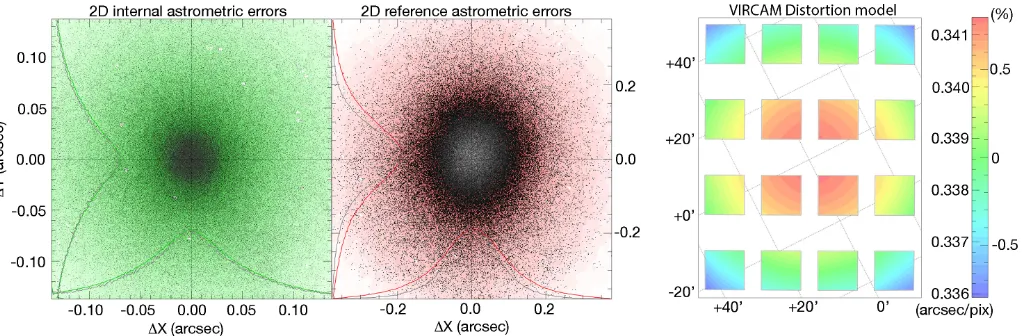
Fig. 8.Verification plots created by Scamp for all data on Orion A in theKSband. Thetwo figures on the leftshow the 2-dimensional internal and external dispersions in the astrometric matching procedure. The symmetry of the Gaussian-shaped distributions indicates that the remaining systematic errors are negligible compared to other noise terms. The typical global errors (rms) were found around 40 mas internally and 70 mas with respect to the reference catalog. Theplot on the righthand sideshows the derived distortion model of VIRCAM, where the color indicates the variation in pixel scale across the focal plane. Only very small distortion levels are seen with an amplitude of∼2% from the center to the edge.

LOOSE8mode offered an unbiased global astrometric solution without any systematics across the focal plane. In principle, the FIX_FOCALPLANE9 mode was also employed successfully, but in that case we observed systematic source clipping toward the outer detectors, resulting in mismatches between individual tiles.

All three bands were calibrated separately with a third-order distortion model over the focal plane. Figure 8 shows the in-ternal (VISTA source-to-source scatter) and exin-ternal (VISTA-to-2MASS scatter) astrometric errors along with the derived VISTA/VIRCAM distortion model as generated by Scamp. The dispersion (rms) for the global astrometric solution in all bands was between 40 and 45 mas with respect to internal source matches and about 70 mas with respect to external (2MASS) matches. This compares very well to the CASU mean rms value of 70 mas as given in the headers of the assembled tiles, which also uses 2MASS as an astrometric reference.

In addition to the astrometric solutions, Scamp can be used to derive photometric scaling factors to calibrate all input data to the same zero point. This method, however, has two major drawbacks: (a) Scamp only calculates zero-point offsets between entire pawprints and does not take residual detector-to-detector differences into account; and (b) Scamp requires single sources to be visible in all input data. The observing strategy, together the sparse focal plane coverage, provides only a tiny overlap-ping field for all telescope pointings. For our jitter box width, we found overlaps smaller than 1 arcmin across. Therefore in most cases there would be no sources available in these overlaps. For these reasons Scamp cannot be used for a global fine-tuned gain harmonization based on relative internal source measure-ments alone. We therefore adjusted the relative zero points by comparing the source catalogs for each detector with 2MASS reference stars (see Sect.3.5.3for details). The typical internal photometric scatter at this stage was around 0.01 mag. For more details on the astrometric properties of our VISTA survey, see AppendixA.2.

8 _{In this mode each detector is treated individually without a global} focal plane model.

9 _{Here Scamp attempts to derive a common WCS projection followed} by computing the median of the detector positions with respect to the focal plane.

3.5. Tile and Orion A mosaic assembly

Prior to assembling the final mosaics, additional processing steps were required to produce science-ready data. These included re-sampling onto a common reference frame, global background modeling, and the fine-tuned gain harmonization. For quality control and computational reasons, we chose to co-add each sin-gle tile before assembling the final Orion A mosaic.

For all co-addition tasks during the data processing, we used the method ofGruen et al.(2014), who implemented an algo-rithm for optimized artifact removal while retaining superior noise characteristics in the co-added frame. In principle this method works in a similar way to aκ −σ clipping technique, but allows for an additional degree of freedom to account for variable point spread function (PSF) shapes. Not only did we observe excellent artifact removal, but also the standard devia-tion in the background was found to typically be 10−20% lower than a median-combined mosaic. The photometric calibrations referred to in the following sections are described in Sect.3.6.

3.5.1. Resampling

With the focal plane model and astrometrically calibrated sci-ence frames in place, the images were resampled onto a common reference frame using SWarp (v2.38.0,Bertin et al. 2002) us-ing a third-order Lanczos kernel (Duchon 1979). To avoid com-plex flux-scaling applications across the tiles due to variable on-sky pixel sizes, we chose a conic equal area projection (COE, Calabretta & Greisen 2002) in equatorial coordinates with one standard parallel atδ=−3◦as the projection type, the field cen-ter to be aligned with the cencen-ter of each tile, and a pixel scale of 1/3 arcsec/pix. Choosing an equal area projection over the standard gnomonic tangential projection assured that every pixel covered the same area on-sky, which avoids further flux adjust-ments for the subsequent photometry.

3.5.2. Global background modeling

the presence of extended emission, this method introduces dis-continuities across the full tiles. To correct for these last remain-ing offsets between overlapping images, we calculated a global background model with the Montage software package10 _while using very large mesh sizes (a constant offset for the tiles N2 and S2 and 1/3 of a detector for all other fields) with SWarp. It is important to note here that despite our efforts to apply as little spatial filtering as possible in the background correction, minor residuals are still visible throughout the assembled tiles. For this reason we do not encourage measurements of nebulous emission on our mosaics. We estimate that structures of few arcminutes in size should mostly be preserved in our reduction.

3.5.3. Illumination correction

Up to this point any zero-point offsets between the detectors were only corrected for during the calibration with the mas-ter flat field. This, however, proved to be mostly insufficient. Unaccounted-for scattered light in the optical train or imperfect flat fields are two examples of effects that can create variable photometric zero points over the field of view. As already men-tioned above, it is not possible to attempt a gain harmonization based on internal photometric measurements from the science fields with VIRCAM owing to the nonexistent overlaps in the offset pattern. The calibration plan offers standard field obser-vations specifically for this correction, but since these measure-ments could not be performed simultaneously with the Orion A field and are carried out only once per night or upon user request, it was safer to rely on external standard catalogs.

To this end, we defined subsets of the data for which we as-sumed stable photometric conditions with respect to the zero point and the PSF shape. Each of these subsets comprised one detector for each jitter sequence (5 frames for the H and KSbands, 3 or 6 frames for theJband; compare with Table2). Thus each tile was split into 96 subsets (16 detectors, 6 offset positions). The jitter box width and the execution time for each of these sequences were in a range where this assumption should hold. This assumption only breaks down for the tiles with offset sky fields (S2 and N2), where one of the six-step offset patterns was completed before any jitter was executed.

The images in each of these subsets were co-added, and for the resulting data we performed source extraction with SExtractor to calculate zero-point offsets relative to 2MASS. We then used the 96 determined zero points to calculate relative flux scaling factors.

3.5.4. Observing parameters

For quality control purposes, we also calculated several ob-serving parameters for each of the given subsets as defined in Sect.3.5.3. These include the local seeing conditions (FWHM; estimated with PSFEx), effective exposure time, frame cover-age, and the local effective observing time (MJD). Most im-portant, aperture correction maps were also generated for aper-tures with discrete radii of 2/3, 1, 2, 3, and 4 arcsec. The fluxes were corrected to an aperture of 5 arcsec for which no variation due to changing seeing conditions was expected. Only point-like sources (as classified by SExtractor) with a high signal-to-noise ratio (S/N) were included in the calculation of the aperture cor-rections. Examples of the quality control parameters are shown in AppendixA.3.

10 _{http://montage.ipac.caltech.edu/}

3.5.5. Co-addition

Once the photometric flux scaling was adjusted with the cor-rect zero-point offsets, the original resampled frames were co-added to the final tiles with SWarp. We then again created shal-low source catalogs and calculated relative zero-point offsets for each tile, and we finally merged all tiles into the Orion A mo-saic. The final mosaic constructed from all data for each filter also features a COE projection with the same standard parallel and pixel scale as the individual tiles. For easier data access and three-color image assembly, we used the same projection for all filters.

Unfortunately, the two separate observations inKSof tile S2 featured one of the best and one of the worst observing condi-tions in terms of image quality (FWHM), respectively. As a con-sequence, when co-adding these tiles, we saw a significant drop in S/N after source extraction. For this reason we decided to only include the data set taken during the better ambient conditions.

3.6. Photometric calibration

The recipes described in this section apply to all stages through-out the data processing where photometric calibration was performed.

3.6.1. Source detection and extraction

Source detection and extraction was performed with SExtractor where we tested several different detection thresholds with re-spect to the background noise level, σ. For the final source catalog we chose a threshold of 1.5σ, requiring at least three connected pixels above this level, while lowering the default de-blending threshold by two orders of magnitude to also detect sources in high-contrast regions. This combination proved to be optimal because a visual inspection of multiple regions in the mosaic showed only a few misdetections (<1%) of nebulosity and residual artifacts. We interpreted the low threshold as a vali-dation of the methods for creating the weight maps and co-added the data. For zero-point determinations and astrometric match-ing, the threshold was typically set to 7σ.

The resulting source catalogs were cleaned by removing all bad measurements, i.e. sources with negative fluxes or a SExtractor flag larger than or equal to four (essentially saturated or truncated objects). For tiles and the final Orion A mosaic cat-alog, we applied the previously determined aperture corrections to all the extracted sources. In addition, each source was also assigned an effective observing MJD, exposure time, frame cov-erage, and local seeing value using the quality control data as described in Sect.3.5.4.

3.6.2. Photometric zero point

subset described in Sect.3.5.3, we typically find several tens of sources matching these criteria. For cross-correlation between the catalogs, we searched for matches within a radius of 1 arcsec where, in cases of multiple possibilities, the nearest match was always selected.

The zero point was determined by applying a one-pass 2σ clipping in the 2MASS −VISTA parameter space and by fit-ting a simple linear function with a forced slope of 1 to the data, weighted by the sum of the inverse measurement errors. Typical errors for the zero point were found to be around 0.01 mag. We also decided not to include color terms in the photometric cali-bration since (a) we did not see any significant dependency on those within the measurement errors; and (b) we aimed for sep-arate calibrations for each individual filter without the need for detections in multiple bands.

3.6.3. Catalog magnitudes

In summary, magnitudes and errors were calibrated onto the 2MASS photometric system (in contrast to the CASU pipeline) and calculated using equations of the form

mi,r=−2.5 log

Fi,r

ti

!

+apcor_i,r+ZPi,r (4)

∆mi,r =1.0857×

p

Ai,rσi,r+Fi,r/g

Fi,r

(5) whererrefers to each aperture size,Fiare the measured fluxes,

ti the exposure times, apcori the aperture corrections, ZPi the

determined zero point, ∆mi the calculated errors, Ai the area

of the aperture, σi the standard deviation of the noise, andg

the gain. We note here that magnitude errors calculated in this way should only be taken as lower limits because (a) SExtractor does not include a term describing the absolute background flux in the aperture typically found in CCD S/N equations and (b) we do not include systematic errors. Furthermore, we do not include uncertainties from the determination of the zero point (typically ∆mZP ≈ 0.01 mag.) for individual source magnitude errors. Since the errors are calculated independently for each source based on photon statistics alone, they can be considered random and may only show spatial correlations due to variable observing conditions and changes in the image quality across the focal plane array.

Finally, the adopted catalog magnitude for each source was chosen so that the selected aperture maximized the S/N among all measurements. After extensive tests, we found that the best overall measurement to represent fluxes for all sources can be achieved by selecting the catalog magnitude from only the two smallest apertures (2/3 and 1 arcsec).

3.7. Final catalog assembly

For the final source catalog, we applied the aforementioned source extraction procedures to the entire Orion A mosaic. In this way, we avoided the issue of multiple detections of the same sources and at the same time increased the S/N in the over-lapping regions. In contrast to all intermediate catalogs, we in-cluded additional processing steps for assembling the final cat-alog of the full Orion A mosaic. We focused on four remaining issues:

1. morphological classification to distinguish between ex-tended and point-like objects;

2. cleaning of spurious detections;

3. sources in the residual nonlinearity and saturation range; 4. source detection near the Orion Nebula due to significant and

highly variable extended emission.

During the following sections we address these supplementary processing steps individually.

3.7.1. Morphological classification

SExtractor itself is able to distinguish between extended and point-like objects on the basis of neural networks. The success-ful application of this method, however, critically depends on the input parameters; in particular, a correct guess of local seeing conditions (FWHM) is crucial. Since the FWHM varies by more than a factor of 2 across the entire Orion A mosaic, the classi-fication with SExtractor shows residual systematics correlating with the variable PSF sizes. To mitigate this situation, we ran SExtractor several times on subsets of the mosaic with similar seeing (see Sect.A.3).

The morphological classification for each source was chosen among all three bands to minimize the effect of the local see-ing. Despite all these efforts, systematic trends are still visible with the SExtractor classification that correlates with observing conditions. Nevertheless, for sources well above the detection threshold, this method produced reliable results.

These issues led us to decide to implement an independent method for distinguishing sources with point-like or extended morphology. We found that a very robust parameter for de-scribing the shape of a source was provided by the curve-of-growth analysis calculated earlier. Since our aperture corrections are only valid for point-like sources (only point-like sources were allowed in its calculation), any elliptically or irregularly shaped source should show a growth value different from 0 in our aperture-corrected magnitudes. Among all available aper-tures, the best parameter for the classification was the difference between aperture corrected magnitudes for the 1 and 2/3 arcsec apertures.

We then cross-matched (1 arcsec radius) all detected sources with the Sloan Digital Sky Survey (SDSS) catalog (DR7, Abazajian et al. 2009), which includes one of the most reliable galaxy classifications in this field down to very faint magni-tudes. From the cross-matched sample, we constructed a rela-tively clean subset by selecting only those sources with mag-nitudes brighter than 23 mag in all available bands (u, g,r,i,z), which seemed to be a good compromise between acceptable S/N and source counts. This subset contained about 47 000 objects, among which about 80% were classified as stars.

Figure9shows the curve-of-growth parameter as a function ofKSmagnitude, with color indicating the corresponding SDSS morphology. Clearly, galaxies separate very well from stars. We then used the cross-matched SDSS subset as a training sample for ak-nearest-neighbor analysis (kNN,k = 30) applied to the entire survey catalog. For details on the classification method and the Python implementation we used, see Pedregosa et al. (2011). In reference to Fig.9, this method tends to favor point-like sources for faint objects simply because the training set in-cluded about four times more stars than galaxies.

Fig. 9.Magnitude growth when increasing photometric apertures from 2/3 to 1 arcsec as a function of KS band magnitude. The color in-dicates the mean SDSS morphology in a box of ∆KS = 0.1 mag, ∆growth=0.02 mag. In this parameter space, galaxies are well sep-arated from point-like objects, which was used for a refined morpho-logical classification.

background galaxies. Unfortunately, SDSS covers only a portion of our Orion A field.

3.7.2. Spurious detections

SExtractor has its own, quite robust, implementation for clean-ing spurious detections by assessclean-ing local detection thresholds for each individual source. These were mostly picked up in the vicinity of bright stars (<∼10 mag) and could be identified well by their morphological classification. To remove these, we used a cleaning radius proportional to the 2MASS magnitude to ap-proximately fit the halo structures and simply removed all ex-tended objects. In addition to this cleaning iteration, we also found a few hundred detections associated with extended emis-sion. This subset, however, was easily identified by large curve-of-growth values, extended SExtractor morphology, and prox-imity to the detection limit. A visual inspection of the remaining sources only revealed very few spurious detections. We did not attempt to remove those manually, since such a task could not have been applied in a consistent manner for the entire mosaic.

3.7.3. Residual nonlinearity and saturation

Comparing the resulting catalog with 2MASS, as displayed in Fig. 10, one can see that stars brighter than a wavelength-dependent magnitude limit were either affected by residual non-linearity problems or were saturated. We therefore replaced all the sources in our catalog that were located in the immediate vicinity of stars brighter than 13, 12, 11.5 mag in J, H,KS in 2MASS, respectively, with the corresponding single clean ref-erence catalog measurement from 2MASS. All clean, high S/N detections (quality flag A) were propagated from the 2MASS catalog. A few remaining very bright sources (quality flagBor worse) can therefore only be found in the 2MASS catalog. Most of them are detections of nebulosity near the ONC and only very few (∼15) are associated with saturated sources. In addition we found about 20 sources in 2MASS withAquality flags across all three bands that are fainter than the above-mentioned limits and were not detected in the VISTA images. These sources were not added to the final catalog.

Fig. 10. 2MASS vs. VISTA photometry. Clearly residual nonlin-earity and saturation effects have an impact on the bright end of the measured magnitudes. For this reason we decided to replace VISION photometry with 2MASS photometry for sources brighter than (13,12,11.5) in (J,H,KS), respectively. The shading indicates source density in a 0.2×0.05 box in this parameter space. The gray line indi-cates a running median with a box width of 0.5 mag, and the dotted hor-izontal line marks the reference value of zero mag difference between the 2MASS and VISTA catalogs.

3.7.4. Sources near the Orion nebula

Common source detection techniques unfortunately do not pro-vide satisfactory results in regions where the background varies significantly on very small scales (i.e., on scales smaller than a few times the size of the core of the PSF). In this case the modeling of the background fails even for advanced methods. The SExtractor method (and also the CASU pipeline) fails for the regions around the ONC where we find background vari-ation on sub-arcsec levels, even when using specialized filter-ing kernels. As a result some localized emission peaks get eas-ily picked up as sources, producing a relatively large number of false detections. We therefore decided to make a 2000×2000 pix (∼11×11 arcmin) cutout around the ONC for which we man-ually cleaned the SExtractor catalogs, while also adding missed sources. All sources in this subset were recentered by calculating a Gaussian least-squares fit at the input coordinates with IRAF (Tody 1986). From this new and cleaned coordinate list, we cre-ated an artificial image with Skymaker (v3.10.5,Bertin 2009) and used this image as input for SExtractor in double imaging mode, while extracting the sources from the original cutout. We note here, that this, of course, does not avoid the problems in the photometry associated with such highly variable background (e.g., flux over- or underestimations depending on aperture ra-dius owing to imperfect removal of the extended emission and systematic offsets in measured source positions). Compared to automated 2MASS photometry that shows many misdetections, we are confident that our source catalog in this region is among the most reliable ones.

4. VISTA Orion A survey data products