Complex fluctuations and robustness in stylized signalling networks

J.

Stat.

M

ech.

(2007)

P01013

ournal of Statistical Mechanics:

J

Theory and Experiment

Complex fluctuations and robustness in

stylized signalling networks

A D´ıaz-Guilera

, A A Moreira

, L Guzman

and

L A N Amaral

1 _{Department of Chemical and Biological Engineering, Northwestern University,}

Evanston, IL 60208-3120, USA

2 _{Departamento de F´ısica Fonamental, Universitat de Barcelona, 08028}

Barcelona, Spain

3 _{Departamento de F´ısica, Universidade Federal do Cear´a, Fortaleza, 2002,}

Brazil

4 _{Unidad Profesional Interdisciplinaria en Ingenier´ıa y Tecnolog´ıas Avanzadas,}

Instituto Polit´ecnico Nacional, M´exico DF, 07340, Mexico

E-mail: albert.diaz@ub.edu,auto@fisica.ufc.br,lguzmanv@ipn.mxand

amaral@northwestern.edu

Received 26 September 2006 Accepted 21 December 2006 Published 16 January 2007

Online atstacks.iop.org/JSTAT/2007/P01013 doi:10.1088/1742-5468/2007/01/P01013

Abstract. Complex fluctuations with correlations involving multiple scales appear in many physical, social and biological systems. In particular, in physiological systems the degree of complexity, measured in terms of the exponent of the time correlations of the fluctuations, is altered with disease and ageing. Here, we show that correlated fluctuations characterized by 1/f scaling of their power spectra can emerge from networks of simple signalling units. We analyse networks of simple signalling units where the type of scaling of the fluctuations is associated with (i) a complex topology with a discrete and sparse number of random links between units, (ii) a restricted set of nonlinear interaction rules, and (iii) the presence of noise. Furthermore, we find that changes in one or more of these properties leads to degradation of the correlation properties. Moreover, changes in the microscopic construction of the model do not produce qualitative changes in the dynamical behaviour, showing hence the robustness of our findings.

J.

Stat.

M

ech.

(2007)

P01013

Contents

1. Introduction 2

2. The model 4

3. System dynamics 6

4. Results 8

5. Robustness 13

6. Discussion 18

Acknowledgments 18

References 18

1. Introduction

A feature of complex physical systems is that they comprise interacting units that communicate among themselves and process external environmental stimuli. The dynamical analysis of these systems is often performed in terms of the time series of some relevant property of the system. Numerous studies have demonstrated that the spectrum of the fluctuations in such time series, i.e. the Fourier transform of the correlation function of the fluctuations, gives a measure of the degree of complexity of the system. Specifically, in complex systems, the behaviour of the system is not a simple superposition of the behaviour of the units but the result of a complicated interrelation between the different units that form it, and the different degrees of complexity are associated with a power-law dependence of the spectrum, which means that correlations span across multiple timescales [1,2].

Complex systems whose fluctuations have correlation holding across multiple timescales are ubiquitous in the social [3] and biological realms [4]. Physiological systems, in particular, generate complex output signals that are scale independent. The complexity of these signals is quantified in terms of the value of the exponent of the power law of the power spectrum of the fluctuations. The range of values of this exponent is related to the physiological conditions, thus in healthy young individuals some observations show a power spectrum such that it scales as the inverse of the frequency, that is, the so-called ‘1/f’ noise; variations in the exponent appear with some pathologies as well as with ageing [5]–[11]. In spite of its practical and fundamental interest [8,12], the origin of such scale-invariant dynamics remains an unsolved problem [13,14].

J.

Stat.

M

ech.

(2007)

P01013

Boolean algebra has been extensively used to model the state and dynamics of complex systems (see [17] for an introduction). The reason such a ‘simplistic’ description may be appropriate arises from the fact that Boolean variables provide good approximations to the nonlinear functions encountered in many control systems [20]–[24]. Indeed, random Boolean networks (RBNs) were proposed by Kauffman [20] as models of genetic regulatory networks, and have also been studied in a number of other contexts [21]–[23], [25]–[28].

In sharp contrast to the inherent stochasticity of RBNs, Wolfram [24] proposed that all real-world complexity might be explained by a class of ordered Boolean networks with identical units, the cellular automaton (CA) models. Interestingly, neither of these two classes of models has been shown to generate the types of complex dynamics with 1/f fluctuations observed, for example, in physiological systems [11,29]. Indeed, in low connectivity RBNs perturbations quickly die out and the system evolves toward an ordered phase, whereas in large connectivity RBNs perturbations propagate to the entire network and the state of the system becomes unpredictable. Similarly, the CA models can only generate periodic or unpredictable/uncorrelated outputs depending on the particular sets of Boolean functions considered [24]. Hence, the construction of a model that could generate complex dynamics with long-range correlations and its alteration with pathology is still very much an open problem [14].

We have recently proposed a new model for the emergence of scale-invariant dynamics in signalling networks [30]. Our modelling approach departs from prior approaches in that we pay especial attention to the topology of the network of interactions. The justification for this focus is that a number of recent studies have shown that the network of interactions in certain living organisms evolves toward a complex structure [18,19]. Our model is rooted in three considerations frequently confirmed in real-world systems:

(i) the units are connected according to a complex topology [19,31,32],

(ii) the interactions among the units comprising the system are nonlinear [17],

(iii) the interaction between the units is affected by noisy communication and/or by external ‘environmental’ stimuli [33].

Of note, we found that combinations of just two of these ingredients are not sufficient to generate 1/f-type signals. In this paper we focus on the robustness of the results reported earlier.

First, we investigate different topological configurations to analyse the relevant ingredients in the construction of the network. Next, we allow some modifications of the way the Boolean functions are implemented and we also let a subset of nodes behave in a different way to the rest of the network. The results reported here enable us to say that all findings in our previous paper are robust in the sense that the appearance of a broad range of responses in terms of the correlation function of the fluctuations is firmly rooted in the considerations exposed above.

J.

Stat.

M

ech.

(2007)

P01013

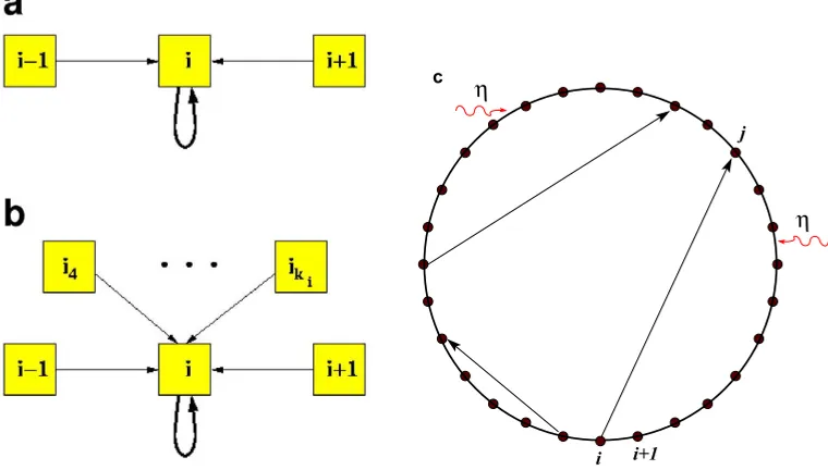
Figure 1. The units forming the system are placed on the nodes of a one-dimensional lattice and establish bi-directional nearest-neighbour connections. With some probability we add long-range unidirectional connections until there are keN such excess links, ke being the average excess connectivity and N the number of units. Each unit processes a set of input signals in the way that is described in the text. The signal received from one of its neighbours is replaced with a random value with probabilityη.

2. The model

In order to study the role of the three factors mentioned above (complex topology, nonlinear dynamics, and noise) in a systematic way we first formalize them mathematically: concerning the system’s topology, we assume the units are placed on the nodes of a one-dimensional lattice and that each unit is bidirectionally connected to its two nearest neighbours. We then increase the topological complexity of the system by adding, with probabilityke, an incoming connection to each node [34] (figure1). The basic

topology we consider is having the units in our system sit on a circle with connections to the nearest neighbours. This is a very regular, ordered (and artificial) network structure. To consider a more general topology we first allow for ‘connection errors’, which we implement through long-range connections to randomly selected units on the circle. This is the so-called ‘small-world’ topology proposed by Watts and Strogatz [18,31]. Although quite stylized, this topology captures some aspects of real-world networks such as (i) the small number of ‘degrees of separation’ between the units and (ii) the local order. Other topological structures will be considered later in the paper.

Concerning the unit’s dynamics, we assume that the state of the units comprising the system is a Boolean variable—Boolean algebra provides a simple way to introduce nonlinearities in the dynamical evolution of the units since it is associated, for example, with threshold input–output relationships. We also assume that the stateσi(t+ 1) of unit

J.

Stat.

M

ech.

(2007)

P01013

σi(t+ 1) =Fi

σi1(t), σi2(t), . . . , σi_ki(t)

, (1)

where ki is the connectivity of unit i—i.e. the number of inputs that unit ireceives—and Fi is a Boolean function (or rule). Note that for a number K of inputs there are 22K

different functions: for example, for K = 3 there are 256 different Boolean functions. The truth table of Boolean functions (or rules) of three-inputs {σi, σi1, σi2 } is of the

following form [16]:

σi1(t) 1 0 1 0 1 0 1 0

σi(t) 1 1 0 0 1 1 0 0

σi2(t) 1 1 1 1 0 0 0 0

σi(t+ 1) b7 b6 b5 b4 b3 b2 b1 b0

(2)

where bj is the output for each of the eight possible combination of inputs, and can take

values of zero or unity. The rules are designated by the decimal number that corresponds to the binary numberb7b6b5b4b3b2b1b0; for example, the Boolean function 11101000 is rule

232 [16,17]. This rule returns as an output the value in the majority among the inputs, and hence it is also named the ‘majority’ rule.

In the following, we will focus our attention on rules that can be generalized to an arbitrary number of inputs. In general, a three-input rule cannot be generalized to any number of inputs. An important class of Boolean rules that is mostly excluded by the generalizable Boolean rules considered above is the class of canalizing functions [16]. In a canalizing rule, the output value of the rule is solely determined by one input, the canalizing variable. Three of the rules we study here are canalizing: 1, 19, and 50. As we shall see, two of these rules lead to a broad range of dynamical behaviour. However, as we will show here, the majority rule, which is not canalizing, also displays a broad range of dynamical behaviours, suggesting that canalizing variables are not necessary to obtain such diverse dynamics.

In order to define the generalizable Boolean functions, we replace the inputs of the neighbours in a three-input rule by an average input σn(t)

σn(t) =

1 + sgn(σi1 +σi2 −1)

2 (3)

where we define sgn(0)≡0; a value of 1/2 for the state σn is what we will call a tie. The

average input σn(t) can be generalized to include an arbitrary number of inputs:

σn(t) =

1 + sgn

2j=ki

j=1 σij−ki

2 . (4)

The Boolean rules of three inputs that are generalizable are symmetric rules that have

b1 =b4 and b3 =b6:5

σn(t) 1 T 1 T T 0 T 0

σi(t) 1 1 0 0 1 1 0 0

σi(t+ 1) b7 b6 b5 b4 b3 b2 b1 b0

(5)

5 _{In this case only it does not matter where the tie comes from, a one on the right and a zero on the left or the}

J.

Stat.

M

ech.

(2007)

P01013

We will keep using the eight-bit decimal representation used for Boolean rules with three inputs to label the corresponding generalizable rule with arbitrary number of inputs [16]. The truth table of a generalizable rule can be simplified as follows:

σn(t) 1 T 0 1 T 0

σi(t) 1 1 1 0 0 0

σi(t+ 1) b5 b4 b3 b2 b1 b0

(6)

where b_i is the output of the function in each of the six different input conditions. This representation, in terms of six possible input combinations, enables a better visual identification of the rules. In the top of figures 4–6 we show the truth tables in this representation of some of the generalizable Boolean functions.

Because of symmetries, there are 26 = 64 independent generalizable rules. However, some of these rules are conjugate rules and we do not need to investigate the whole set of rules. Two conjugate rules will have identical dynamics if the zeros and ones are switched for one of them [16]. Additionally, some rules are self-conjugates. These are rules 23, 51, 77, 105, 150, 178, 204, and 232. Self-conjugate rules have an inverse rule. Two rules are said to be inverse if, when both starting with the same initial condition, they will be in exactly the same state every other time step and in the inverse state for the other time steps. An example of inverse rules is given by rules 204 (the ‘identity’ rule) and 51 (the ‘negation’ rule). The identity rule will keep the initial state, whereas the negation rule will switch between the initial state and its inverse. Other pairs of inverse rules are {23, 232}, {77, 178}, and {105, 150}.

The final ingredient of our model is the existence of noise. We introduce noise in the dynamics by assuming that a unit has a probability η of ‘reading’ a random Boolean variable instead of the ‘true’ state of the neighbour. This noise is intended to mimic two effects that are always present in living processes: (i) communication errors due to the intrinsic noise fromin vivo conditions, and (ii) external stimuli affecting the transmission of signals to a unit [33].

It is important to note that in our model the noise acts only on the inputs of the neighbours of a unit. This implies that the state of a unit is not changed because of noise only. Moreover, because a unit processes the average state of all neighbours, the disturbance caused by the noise is not as large as one would estimate based on the fact that the noise can produce a change in an input from zero to one orvice versa.

3. System dynamics

In our analysis of the dynamics of the model, we define the state S(t) of the system as the sum of the states of all the units

S(t) =

i

σi(t). (7)

J.

Stat.

M

ech.

(2007)

P01013

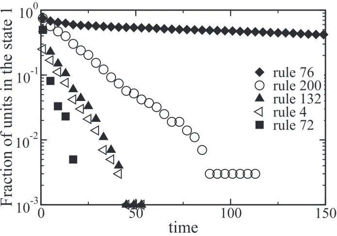
Figure 2. Convergence to a fixed state. For some Boolean rules, whenever a unit is in the inactive (0) (or active (1)) state it will remain in this state for the next time step. Because in the model we do not allow for noise on the value a unit reads from itself, networks of units evolving in accordance with these rules will always converge to a fixed state with all units in the 0 state. (Note that for the conjugate rules the ‘absorbing’ state would be all units in the 1 state.) The time needed to reach this fixed state depends on the particular rule; while for rule 76 it takes several thousand steps to converge to the fixed state, rule 128 (data not shown) requires fewer than ten time steps and rule 0 (data not shown) requires two time steps.

Even in the presence of noise, not all of the 64 generalizable rules that we consider will display fluctuating time series. For example, rules 0, 4, 72, 76, 128, 132, and 200 converge to a fixed state, in which all units are in state zero (see figure 2). Additionally, the output of rules 51 and 204 depends only on the state of σi, so it will not be affected

by noise either and, as such, will not display fluctuations either.

Because of these facts and because conjugate rules have identical dynamics, we need to investigate only 24 of the 64 generalizable rules. These rules are 1, 5, 18, 19, 22, 32, 33, 36, 37, 50, 54, 73, 77, 90, 94, 104, 105, 108, 122, 126, 146, 160, 164, and 232. This process of elimination of irrelevant rules is schematized in [30].

To analyse the character of the fluctuations we apply the detrended fluctuation analysis (DFA) method to the time series generated by the model [7,35]. In this method, the first step is to integrate the original time series. Then, the integrated time series is divided into ‘boxes’ of size n and, for each box, a least-square linear fit is performed. Next, the root-mean-square deviation of the integrated time series from the fit, F(n), is calculated. This process is repeated over different box sizes or timescales.

J.

Stat.

M

ech.

(2007)

P01013

quantifies long-range time correlations in the dynamical output of a system by means of a single scaling exponent α.

Brownian noise yields α = 1.5, while uncorrelated white noise yields α = 0.5. For a number of physiological signals from free-running, healthy, mature systems, the scaling exponent α takes values close to one, so-called 1/f-behaviour, which can be seen as a ‘trade-off’ between the two previous limits [11]. The exponentαis related to the exponent

βof the power spectrum of the fluctuations,S(f)∼1/fβ_{, through the relationβ = 2α−1.}

In many physiological signals, the scaling properties represented by means of the value of one scale-invariant quantity suffer changes along with the dynamical evolution of the system. For instance, heart interbeat dynamics under healthy conditions display long-range correlations with fractal scaling expressed through a single scaling exponent (α≈1) [11]. In contrast, a breakdown in the scaling properties is observed for situations such as heart failure and ageing [7,11,36].

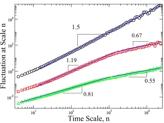
This change from one to two or more scale-invariant exponents in the description of the system has been described as the loss of fractal organization during the evolution. In our simulations (with all units operating with Boolean rule 232), we observe that three distinct values of ke lead to quite different dynamics of the system (figure 3). For a

small value ofke, the time correlations are similar to those of Brownian noise with a single

scaling exponent in the interval 4< n <105_{. Of interest, for intermediate values ofk} etwo

main exponents are observed which lead to two scaling regions; for small and intermediate scales the scaling exponent is close to unity, indicating long-range correlations as in the 1/f-noise; for large scales the scaling exponent is close to α≈0.5, which resembles white noise dynamics. For large values of ke, the dynamics is also similar to white noise, that

is, almost uncorrelated, and a weak crossover behaviour is observed.

As we can see in figure 3 the crossover of the exponent α to a lower value happens at relatively large scales. We have exhaustively checked the time series for the generated data and we have verified that there exists a range of time box sizes (40 < n < 4000) in which the scaling of the fluctuations with n follows a straight line, thus defining a unique value of the exponent. For this reason, we are going to systematically estimate the exponent α within this region.

4. Results

Prior to presenting our results it is worthwhile to note that both the RBN and CA models can be seen as limiting cases of the present model in the absence of noise: an RBN model corresponds to a completely random network with different Boolean rules for the units, while a CA model corresponds to ke = 0 and all units evolving according to the same

rule.

In principle, we consider systems whose units all evolve according to the same rule, as in CA models. We systematically study the 24 different Boolean functions of three inputs which do display fluctuations, for different pairs of values of ke and η. In figures 4–6we

J.

Stat.

M

ech.

(2007)

P01013

Figure 3. Plot of F(n) versus nfor sequences of the state of Boolean signalling networks. We show the detrended fluctuation analysis for three cases with N = 4096 units; Fi = 232; η = 0.15; and ke = 0.15, ke = 0.45, and ke = 0.9 (from top to bottom curves). The three values ofke lead to different dynamics of the system as is observed in the plots. For a small value of ke the system displays short-range correlations as in Brownian noise; furthermore, we observe a single scaling exponent in the range 10< n <104. For intermediate values of ke, long-range correlations are observed in the range 10< n <103 with a scaling exponentα≈1 as in the 1/f-noise. In this particular case we observe a crossover behaviour in the scaling exponent; for short scales (10< n < 103_{) the exponent} is close to unity whereas for large scales (103 < n) the scaling exponent is close to the white noise value. For a large value ofkethe evolution is almost uncorrelated but with a weak crossover in the scaling exponent.

dependence on the excess connectivity. Finally, see figure 6, there is a collection of rules for which fluctuations are always uncorrelated.

Some of the described rules have a clear physiological meaning. As a representative of the first set, rule 232 is a majority rule, that is, a unit will be active in the next time step only if the majority of its neighbours, including itself, is active currently, and vice versa. On the other hand, rule 50, representative of the second class, is a threshold rule with refractory time period; that is, whenever the inputs of the neighbours surpass a certain value a unit becomes active in the next time step and then will be inactive for at least one time step.

Particularly interesting are the results for rule 232, the majority rule (see [23] for applications of this rule to other contexts). Interestingly, we find three distinct types of behaviour (figure 3): for small ke, we find mostly Brownian-like scaling. For largeke, we

find mostly white-noise dynamics. Of greatest interest, for intermediate values ofke and

J.

Stat.

M

ech.

(2007)

P01013

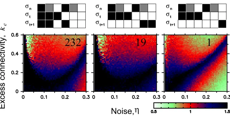
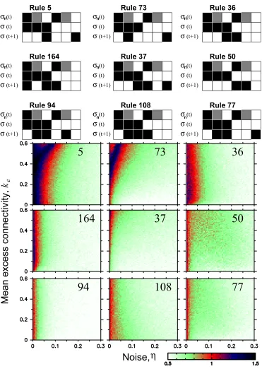
Figure 4. Truth table and phase space for signalling networks with units obeying rules 232, 19, and 1. In the truth tables, black represents one, grey represents tie and white represents zero. In the phase spaces, we use the colour scheme shown in the bar to indicate the value of the scaling exponentα characterizing the auto-correlations in the dynamics of the system by means of the detrended fluctuation analysis method [7]. The exponent is systematically estimated for timescales 40 < n <4000. We show α for 61×61 pairs of values ofke and the noiseη in the communication between the units comprising the network. For all simulations, we follow the time evolution of systems comprising 4096 units for a transient period lasting 8192 time steps, and then record the time evolution of the system for an additional 10 000 time steps. In order to avoid artifacts due to the fact that for some of the rules the units switch states with period 2, we consider in our analysis the state of the systems at every other time step. The rules shown in this figure display different types of noisy fluctuations depending on the values of η andke. For all three rules, the system generates 1/f-noise for a broad range of noise intensities.

One interesting question raised by these results is how a single rule can generate such a broad range of behaviours.

First, we focus on the Brownian noise behaviour observed for small excess connectivity. In the limiting case of a regular ring andη = 0 the system evolves toward a stable configuration with fixed width bands—or clusters—of units in the same state. As

η increases, the boundaries between the clusters fluctuate in time. For smallke, the effect

of the random links is merely to increase the effective value ofη. In such a situation, the state of the system changes by small amounts because only the units at the boundaries between clusters can change value. Hence, the changes in S(t) are uncorrelated random variables and the dynamics are Brownian (see [30] for more details).

Next, we focus on the white noise behaviour observed for large ke. If ke is large,

J.

Stat.

M

ech.

(2007)

P01013

Figure 5. Truth table and phase space for networks with units obeying rules 5, 36, 37, 50, 73, 77, 94, 108, and 164. These rules can generate complex fluctuations only for small intensities of the noise. Curiously, for these rules, the dynamics show a very weak dependence onke.

Finally, we focus on the 1/f behaviour observed for intermediate values of ke. Our

J.

Stat.

M

ech.

(2007)

P01013

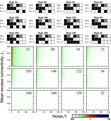
Figure 6. Truth table and phase space for networks with units obeying rules 18, 22, 32, 33, 54, 90, 104, 105, 122, 126, 146, and 160. These rules are only able to generate white noise fluctuations.

a large number of interacting units [37]. However, these results were based on a situation similar to the case of large excess connectivity. For intermediate values ofke, the number

of random connections remains small enough that order is not destroyed—i.e., clusters can still form—but large enough that information can be transmitted to distant parts of the system quite rapidly. The fact that local information from one part of the system is ‘broadcast’ to all scales is the mechanism by which long-range correlations and 1/f

behaviour are generated.

J.

Stat.

M

ech.

(2007)

P01013

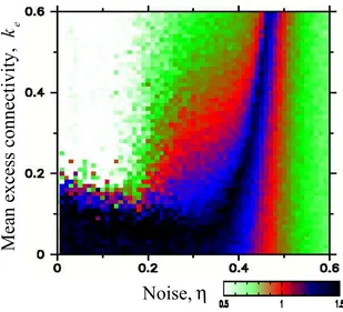
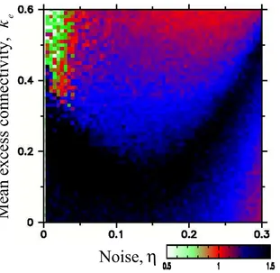
Figure 7. Phase space for signalling networks. Here we consider that initially each unit is connected to its two nearest neighbours (±1) and to its two next nearest neighbours (±2), before adding the extra connections. The systems consist of units operating according to the majority rule. We used the same parameters as in figures4–6 and each value is an average over five independent runs.

our approach, making the system response completely unpredictable and the fluctuations have a white-noise character (see [30]). This can also be inferred from figure 10 in the next section, when increasing the fraction of random rules with respect to a fixed one.

5. Robustness

In order to determine the generality of the results presented above, one needs to address the question of how these findings are affected by (i) changes in the topology of the network, and (ii) changes in the units’ implementation of the rules. Since from both a physiological and a physical point of view the majority rule has a meaningful interpretation, we take it as a starting point, but it is worth noting that it could be performed for any of the ‘complex’ rules represented in figure 4 (rules 19 and 1).

J.

Stat.

M

ech.

(2007)

P01013

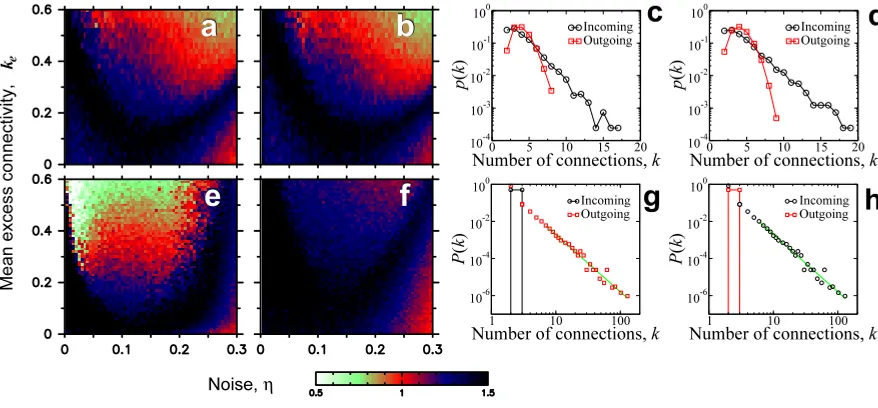
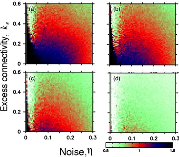
Figure 8. Phase space ((a), (b), (e), (f)) for signalling networks with units operating according to rule 232 and their corresponding distributions of number ki of connections of the units ((c), (d), (g), (h)). Top: case of networks in which the units have connections with theirki>2 nearest neighbours, whereki follows an exponential distribution with (a) mean 2.5 and (b) mean 3. We then addke unidirectional links per unit between pairs of randomly selected units. Bottom: thekeN additional unidirectional links are not between pairs of randomly selected units, but instead between units selected according to preferential attachment— which is known to generate power-law decaying distributions of ki [19]. We consider two distinct situations: (e), (g) the preferential attachment rule is used in selecting the unit sending the outgoing link while the unit receiving the incoming link is selected at random, and (f), (h) the preferential attachment rule is used in selecting the unit receiving the incoming link while the unit sending the outgoing link is selected at random.

In the first case, we consider as initial set-up a one-dimensional array in which each unit ihas bidirectional connections to its nearest neighbours (±1) and to its next-nearest neighbours (±2). In figure7we see that the inclusion of two additional neighbours before we add the extra connections leads to a similar structure of the phase space and the three different regimes are still observed. It is clear, however, that more noise intensity is needed to obtain the regimes observed in the original system with only nearest neighbours (see figure 4 (left)).

Finally, we note that the network topologies considered so far span the cases of ordered one-dimensional lattices, small-world networks, and random graphs [38]. However, all networks considered are comprised of units with approximately the same degree, i.e. the same number of connections. To investigate the role of the distribution of number of connections, we also study networks which span the range of empirically observed degree distribution: a delta-distribution, an exponential distribution, and a power law distribution. The latter case corresponds to the so-called scale-free networks [19].

J.

Stat.

M

ech.

(2007)

P01013

Figure 9. Phase space with mixing of simple majority and clear majority rule. We calculate the correlation exponentα for systems composed of units operating according to rule 232 but with one-quarter of the units operating according to a clear majority rule. We observe that the phase space displays mostly Brownian and 1/f noise.

we consider distributions of number of incoming and outgoing connections for networks with exponential distribution of local links with different means. Allowing the number of incoming connections to fluctuate also changes the distribution of number of outgoing connections, which becomes a Poisson distribution. The figures demonstrate that the change in the increased number of local connections considered in panels (a) and (b) leads to no significant change in the results. The reason is that the complex dynamics are generated at the boundary between domains: when one allows some units to have more local connections, these units still have the same number of units to the left and to the right, so the existence of a single long-range connection is enough to destabilize the boundary.

J.

Stat.

M

ech.

(2007)

P01013

(a)

(b)

(c)

(d)

(a) (b)

(c) (d)

Figure 10. Phase space for signalling networks with mixing of Boolean rules. We systematically calculate the exponent α, characterizing the correlations in the dynamics, for systems composed of units operating according to rule 232 but with some fixed fraction of units operating according to a randomly selected symmetric Boolean rule. Each value is an average over five independent runs. (a) 1/16 of the units operating according to a randomly selected rule. (b) One-eighth of the units operating according to a randomly selected rule. (c) One-quarter of the units operating according to a randomly selected rule. (d) One-half of the units operating according to a randomly selected rule.

long-range connections [39]. In contrast, a power law distribution of incoming links does

lead to a change in the phase space of dynamical behaviours. The reason may be that, since information travels only one way on the connections, the fact that some units are receiving so many of the long-distance connections will make it harder for the system to reach the small-world regime.

The second class of change we have considered is the way in which the units implement the rules. We look at this from two different perspectives: one consists in restricting the majority rule to need more than the simple majority and the second in allowing a subset of units to operate according to another rule, which accounts for the effect of ‘errors’ in the units’ implementation.

J.

Stat.

M

ech.

(2007)

P01013

Figure 11. The same as figure 10 but a fraction of nodes operate according to rule 50 instead of a random rule. (a) 1/16 of the units operating according to rule 50 and 15/16 operating according to rule 232. (b) One-eighth of the units operating according to rule 50 and seven-eighths operating according to rule 232. (c) One-quarter of the units operating according to rule 50 and three-quarters operating according to rule 232. (d) One-half of the units operating according to rule 50 and one-half operating according to rule 232.

the state. In this way we have a more restrictive majority rule, that is, a unit would remain in its initial state unless a clear majority operates. We perform simulations to evaluate the correlation exponent for systems with a fraction of units operating according either to a clear majority or simple majority rule. The use of a clear majority rule forces the units to remain in their state for more extended periods before switching to the opposite state. The phase space shows the same regimes as in figure 4 (left) but a more extended region corresponding to Brownian dynamics is observed (figure9).

We also investigate the effect of allowing the co-existence in the system of distinct Boolean rules. To this end, we first explore systematically the existing dynamical behaviours in the phase space defined by (ke, η) for systems composed of units operating

J.

Stat.

M

ech.

(2007)

P01013

1/f, and Brownian noise (figure10). Specifically, if more than one-quarter of all the units operate according to randomly selected Boolean functions, then the phase space displays mostly white noise dynamics.

Additionally, we explore systematically the existing dynamical behaviours in the phase space defined by (ke, η) for systems composed of units operating according to either rule

232 or rule 50. When both rules are present in the system (and at least 50% of the units operate according to rule 232) we still find several distinct classes of dynamical behaviours, including a wide range of parameter values that generate 1/f noise (figure 11).

6. Discussion

Our results are significant for a number of reasons. First, we propose a new model for signalling systems that generates a broad range of behaviours reminiscent of those observed in physiological systems. Second, we demonstrate that such a broad range of behaviours can only emerge under a number of restrictive, but realistic, assumptions. Namely, the system must have a complex topology, its components must interact in a nonlinear fashion and according to a very specific type of interaction, and must be robust in the presence of noise. Third, our findings suggest that two classes of models that have received much attention for over three decades—random Boolean networks and cellular automata— cannot generate the types of complex dynamics observed in physiological systems [11,29]. We find that the character of the phase space does not depend on the distribution of the number of connections. Moreover, different distributions of incoming or outgoing links do change the shape and location of the region with specific time correlations but do not change the fact that distinct classes of dynamical behaviours are observed. This is suggestive of universal behaviour.

Another interesting question raised by our results relates to the natural selection of a few interaction rules out of all possible such rules. One may speculate that in an evolutionary process in which connections are created and destroyed units not interacting through the rules that generate other most complex adaptive behaviours would eventually become disconnected from the system, leading to a situation in which just a few rules are observed.

Acknowledgments

We thank A Arenas, J J Collins, L Glass, R Guimera, I Henry, C-C Lo, G Moody, J M Ottino, C-K Peng, C J Perez, M Sales-Pardo, H E Stanley, and G Weisbuch for stimulating discussions. LANA thanks a NIH/NIGMS K-25 award and the JS McDonnell Foundation. AD-G acknowledges financial support from the Spanish Ministerio de Educaci´on, Cultura y Deporte, DGES (Grant No BFM2003-08258), European Commission—Fet Open project COSIN IST-2001-33555, and Generalitat de Catalunya (2005BE00446).

References

[1] Govindan R B, Vyushin D, Bunde A, Brenner S, Havlin S and Schellnhuber H J, 2002Phys. Rev. Lett.

89028501

J.

Stat.

M

ech.

(2007)

P01013

[3] Takayasu H (ed), 2002Empirical Science of Financial Fluctuations(Tokyo: Springer) [4] Shlesinger M F, 1987Ann. New York Acad. Sci.504214

[5] Bassingthwaighte J B, Liebovitch L S and West B J, 1994Fractal Physiology (New York: Oxford University Press)

[6] Malik M and Camm A J (ed), 1995Heart Rate Variability(Armonk, NY: Futura) [7] Peng C K, Havlin S, Stanley H E and Goldberger A L, 1995Chaos582

[8] Hausdorff J M, Purdon P L, Peng C K, Ladin Z, Wei J Y and Goldberger A L, 1996J. Appl. Physiol.

801448

[9] Ivanov P C, Amaral L A N, Goldberger A L, Havlin S, Rosenblum M G, Struzik Z R and Stanley H E, 1999Nature399461

[10] Amaral L A N, Ivanov P C, Aoyagi N, Hidaka I, Tomono S, Goldberger A L, Stanley H E and Yamamoto Y, 2001Phys. Rev. Lett.866026

[11] Goldberger A L, Amaral L A N, Haussdorf J M, Ivanov P C, Peng C K and Stanley H E, 2002Proc. Nat. Acad. Sci.99(Suppl. 1) 2466

[12] Marshall J C, 2000Crit. Care Med.282646

[13] Abbott D and Kish L B (ed) 2000Unsolved Problems on Noise 1999 (AIP Conf. Proc. no511) (Melville, NY: American Institute of Physics)

[14] Chialvo D R, 2002Nature419263

[15] Kauffman S A, 1993The Origins of Order: Self-Organization and Selection in Evolution(Oxford: Oxford University Press)

[16] Wolfram S, 1994Cellular Automata and Complexity: Collected Papers(Boulder, Colorado: Westview) [17] Kaplan D and Glass L, 1997Understanding Nonlinear Dynamics(Berlin: Springer)

[18] Strogatz S H, 2001Nature410268

[19] Albert R and Barab´asi A L, 2002Rev. Mod. Phys.7447 [20] Kauffman S A, 1969J. Theor. Biol.22437

[21] Weng G, Bhalla U S and Iyengar R, 1999Science28492 [22] Albert R and Barab´asi A L, 2000Phys. Rev. Lett.845660

[23] Aldana M, Coppersmith S and Kadanoff L P, 2003Perspectives and Problems in Nonlinear Science. A Celebratory Volume in Honor of Lawrence Sirovich(Springer Applied Mathematical Sciences Series) ed E Kaplan, J E Marsden and K R Sreenivasan (Berlin: Springer)

[24] Wolfram S, 2002A New Kind of Science(Champaign, IL: Wolfram Media)

[25] Moreira A A, Mathur A, Diermeier D and Amaral L A N, 2004Proc. Nat. Acad. Sci.10112085 [26] Moreira A A and Amaral L A N, 2005Phys. Rev. Lett.94218702

[27] Klemm K and Bornholdt S, 2005Phys. Rev.E72055101 [28] Shmulevich I and Kauffman S, 2004Phys. Rev. Lett.93048701 [29] Lipsitz L A, 2002J. Gerontol.A57B115

[30] Amaral L A N, D´ıaz-Guilera A, Moreira A A, Goldberger A L and Lipsitz L A, 2004Proc. Nat. Acad. Sci.

10115551

[31] Watts D J and Strogatz S, 1998Nature 393440 [32] Koch C and Laurent G, 1999Science28496

[33] Mar D J, Chow C C, Gerstner W, Adams R and Collins J J, 1999Proc. Nat. Acad. Sci.9610450 [34] Newman M E J and Watts D J, 1999Phys. Lett.A263341

[35] Taqqu M S, Teverovsky V and Willinger W, 1995Fractals3785

[36] Iyengar N, Peng C K, Morin R, Goldberger A L and Lipsitz L A, 1996Am. J. Physiol.271R1078 [37] Glass L and Hill C, 1998Europhys. Lett.41599