Bundling as a Leverage Device in Quality Differentiated Duopolies with Home Markets

Bundling as a Leverage Device in Quality

Differentiated Duopolies with Home Markets

Jan Kr¨amer

September 3, 2007

Abstract

Digital convergence of telecommunication and entertainment media ser-vices drove former network monopolists into a prisoner’s dilemma forcing them to enter each others markets. In this reciprocal duopoly firms now offer their services in a bundle - commonly known as Triple Play. I investigate whether bundling is indeed a profitable pricing strategy for these services and if it can facilitate market power leverage. I will show that bundling serves as a powerful leverage device for one firm in this industry. This is achieved through a quality sorting effect accruing as the firms wish to shield themselves from increased price competition in the market for bun-dles. Thereby, one firm emerges as the high-quality, high-profit provider in both markets, whereas the competing firm has to settle for low qualities and profits. Finally, I show that bundling raises not only producers’ but also consumers’ welfare.

Keywords: digital convergence, bundling, market power leverage, vertical differentiation, multi-market competition

JEL classification: L13; L86; M21

∗_{The author is affiliated with the Institute for Economic Theory and Operations Research,}

1

Introduction

Digital Convergence has revolutionized the entire telecommunication and enter-taining media industry. In Germany, for example, today former telecommuni-cation monopolist Deutsche Telekom AG offers not only internet and telephony services over her network, but also digital TV (IPTV). On the contrary, TV broad-casters, such as regional cable network monopolists, have also invested in network digitization in order to augment their product portfolio by a telephony and internet service themselves. From a more theoretical perspective, digital convergence has created a prisoner’s dilemma which forced these companies to enter each others markets: Each firm finds it profitable to capture a share of the competitor’s market and hence no one can commit not to do so. Consequently, both firms will enter each others markets, a structure which I refer to as a reciprocal duopoly because monopolies have transformed into duopolies through reciprocal entry. The pecu-liar feature of this market structure is that each firm originates from ahome market

where it is considered to have some additional market power over her competitor.1 Moreover, it is widely believed that each firm’s home service (i.e. telephony and web access for the telecommunication firm and TV for the cable provider) is superior to that of the competitor’s, e.g. in terms of reliability, customer service, transfer speeds, video quality or content. Although the observed product differ-entiation might also be due to a rather technical nature at first, I argue that there is also a long-lasting economic intuition which will prevail even if technical diffi-culties should be overcome in a matured industry. More precisely, I consider this industry to be vertically differentiated, such that firms may deliberately choose different service qualities in order to weaken price competition. Each firm will then make use of its home market advantage by offering a service quality higher than that of its competitor, because high-quality products are generally associated with higher profits.

In practice providers often employ an additional business strategy which has become known under the buzz word Triple Play: That is, firms often sell their services in a bundle only, although it would be technically possible to offer each service separately. For example, if a customer wants to use the cable company’s telephony service he will also have to sign up for a TV contract - the firm’s home product. Likewise, Deutsche Telekom makes the provision of its IPTV service conditional upon the purchase of its telephony service.

In this article, I will investigate whether bundling is indeed a profitable pricing strategy and under which circumstances it might be part of an equilibrium strat-egy. My main result is that bundling serves as a powerful market leverage device through which one firm may carry its home market advantage over to the

ondary market. This is achieved through a quality-sorting effect which emerges as firms seek to detensify price competition by specializing on providing either the high- or low-quality service in both markets, thereby leaving the high-end provider better and the low-end competitor worse off than under separate selling. Furthermore, I can show that this result is robust with respect to different cost functions, as long as the costs of service quality stem from fixed costs mainly.2

More specifically, I consider a three-stage game in which firms first choose their pricing strategy (i.e bundling or separate pricing), then decide upon their service quality levels in all markets and finally compete in prices. Thus, this paper relates to two major strands of economic literature: vertical product differentiation and bundling.

The basic structure of the game employed here, where firms in a duopoly decide first on quality levels and then on prices, owes much to Shaked and Sut-ton (1982, 1983).3 These early contributions derive consumers’ quality choice from a direct utility function relating different preferences to differences in in-come. Instead, Tirole (1988, Section 2.1.1) considers an indirect utility function, which introduces a heterogeneous taste parameter that can be interpreted as the marginal rate of substitution between income and quality. Thus, higher income corresponds to higher taste for quality and in this vein Tirole was able to cap-ture the notion of the earlier papers by the same simple (indirect) utility function which I will employ here.4 _{These classical contributions have all affirmed that}

in equilibrium firms will differentiate their products and that the firm producing the higher quality will earn greater profits than the low-quality provider.5 As Lehmann-Grube (1997) points out, thishigh-quality advantage is hardly surpris-ing, since all authors have assumed either zero or small and decreasing costs of quality improvement. Although, subsequently some authors (Ronnen 1991; Motta 1993; Boom 1995; Aoki and Prusa 1996) have confirmed the high quality advan-tage for specific cost functions, Lehmann-Grube is able to generalize this result to all cost functions which are increasing and convex in the quality chosen, but

in-2_{This seems to be a natural assumption in the context of network industries, where scale}

eco-nomics are rather prominent since each additional customer induces near zero marginal costs, whereas (fixed) costs of e.g. network maintenance are very high. A related argument justifies to focus on a two-firm economy because high sunk costs constitute an insurmountable entry barrier to firms not controlling a network of their own.

3_{Previous work on vertical product differentiation has either assumed qualities as exogenous}

(Gabszewicz and Thisse 1979) or focused on non strategic market structures (Mussa and Rosen 1978).

4_{See also Peitz (1995) for a more elaborate argument. Therein Peitz constructs the}

correspond-ing direct counterpart of Tirole’s indirect utility function and shows that the underlycorrespond-ing preference relation satisfies reflexivity, transitivity, completeness and local nonsatiation.

dependent of the output.6 _{Furthermore, he shows that if firms choose their quality}

sequentially in Stackelberg fashion, then the Stackelberg leader will always se-lect the product of higher quality. This result is important for the present context because it explains that the incumbent can exploit its home market advantage by establishing itself as the high-quality provider.

The literature on bundling, on the other hand, has at first been primarily con-cerned with monopolized markets. The seminal papers of Adams and Yellen (1976), McAfee, McMillan, and Whinston (1989) and Schmalensee (1982, 1984) highlighted bundling as a price discrimination device for multi-product monopo-lists. Later, Whinston (1990), in an effort to reestablish the previously discred-ited leverage theory,7 considered a market structure in which a multi-product firm holds a monopoly in one product market, but faces imperfect competition in the other. With some noticeable exceptions this basic market structure has subsequently been in the focus of attention and by it scholars have shown vari-ous means through which bundling may facilitate market power leverage. Among these were entry deterrence (Whinston 1990; Martin 1999; Carlton and Waldmann 2002; Nalebuff 2004), economics of aggregation (Bakos and Brynjolfsson 2000), cost savings (Chae 1992; Salinger 1995; Bakos and Brynjolfsson 1999), infor-mational leverage (Choi 2003), reduction of rivals’ innovation incentives (Choi 2004), (tacit) collusion (Seidmann 1991; Spector 2007) and competition mitiga-tion (Carbajo, de Meza, and Seidmann 1990; Whinston 1990; Chen 1997). In this paper, I show that bundling might also achieve market leverage through aquality sorting mechanism.

I deviate from Whinston’s standard market structure by assuming a duopoly in both markets. This assumption is per se not new to the bundling literature (c.f. Matutes 1992; Anderson and Leruth 1993; Economides 1993; Kopalle, Krishna, and Assuncao 1999),8 _{even in the context of the Triple Play industry (Reisinger}

2006; Diallo 2006). In my model, however, each firm has a home market in which it enjoys a strategic advantage. Moreover, none of the above analyses is con-cerned with market leverage since each firm’s market power is lessened consider-ably when its primary market is a duopoly. Also in my setting, ex-ante it is not

6_{On the contrary, if quality improvement induces an increase ofmarginal cost (at a higher rate} than consumer’s willingness to pay) Moorthy (1988) affirms that the low-quality provider earns greater profits.

7_{In a nutshell, theleverage hypothesis suggests that a firm with market power in its primary} market could use bundling as a device in order to gain an advantage in a secondary market. The hypothesis has for a long time been dismissed on the grounds of theChicago critique (cf. e.g. Director and Levi 1956; Bowman 1957; Posner 1976), which, however, implicitly assumed a perfectly competitive secondary market and constant returns-to-scale technology.

8_{These papers have mainly investigated whether pure bundling (offering just the bundle) or}

clear whether bundling may facilitate market leverage because the leverage efforts of either firm counteract. Nevertheless, I can show that the quality sorting mech-anism of bundling is powerful enough to serve as a leverage device in vertically differentiated industries, even is market power is rather limited.

The remainder of this article is structured as follows. Section 2 will introduce the formal model which serves as the basis of my analysis. In particular, I will consecutively derive equilibrium conditions for the separate selling- and bundling regime and eventually deduce the equilibrium selling strategy of each firm. In Section 3 I will briefly consider the welfare effects of bundling and, to conclude, comment on the results in the light of the leverage theory and future research in Section 4.

2

The Model

2.1

Principal Assumptions and Game Structure

There are two established firmsi= 1,2in the industry whose home (or primary) markets are denoted by m = A, B, respectively. For the main part of the model, I assume that firms have already entered each other’s home markets (reciprocal entry) and offer exactly one service for each market.9

Game Structure: Recall that the aim of my model is to show that one firm can quality leverage its home market advantage over to its secondary market by employing a bundle pricing strategy. To this extend, consider the following three-stage game: In the first three-stage, firms decide whether to sell their services as a pure bundle or separately. For now, I assume sequential decision making, where one firm may observe the other firm’s pricing strategy. In the second stage of the game, firms choose whether they will offer a high- or low quality service for each market, where quality levels are exogenously given byqH ≥4qL >0.10 Finally,

in the third stage, firms simultaneously set prices p ∈ _R+_{. The solution concept}

is that of subgame perfectness (Selten 1975).

Notice that the game structure reflects that quality is rather a long term variable which cannot be altered so quickly. Although under facilities-based competition

9_{More specifically I take the firms’ entry decision as given and sunk, such that exit is}

pro-hibitively costly. Thus, I fade out any aspects related to strategic entry deterrence nor will I further address the question on whether entry should have occurred in the first place.

10_{The choice ofq}

H ≥4qLwill be motivated later in the text and is not crucial for the quality

firms have maximal control over the network and associated quality characteris-tics, once a decision has been made, e.g. with respect to a certain technology, con-siderable sunk costs constitute a high level of quality commitment. Hence, once firms have made a quality decision (in stage two of the game), this decision is sunk and irrevocable during the price competition (stage three). Furthermore, the main aim of the present model is to investigate the long term impact of bundling as a pricing strategy decision upon the firms’ quality decision and subsequent price competition. In this mindset, the pricing strategy decision must take place before the quality decision, i.e. before the quality decision has become sunk.

For the further presentation of the model, it will be convenient to introduce a short-hand notation distinguishing between the four subgames which may emerge after the first stage of the game. In particular, denote by ss the subgame where both firms choose separate pricing,sb the subgame where firm 1 chooses separate and firm 2 bundle pricing,bs the subgame where firm 1 chooses a bundle pricing and firm 2 a separate pricing strategy, and finally,bb, where both firms choose the bundle pricing strategy. Moreover, I will denotess as theseparate pricing regime, and all other subgames asbundle pricing regimes.

Home Market Advantage: It is at the heart of this model for each firm to have a home market in which it can exercise some additional market power over her competitor. A first-mover-advantage seems to capture this very adequately. In-deed, the incumbent has been in the market before and should therefore be able to decide upon his service quality prior to the entrant. In this case, a standard result of the vertical differentiation literature is that the first-mover will choose to provide the high-quality service, because it is associated with the higher rev-enues, whereas the entrant has to settle for the low-quality, low-revenue service (high-quality advantage principle). When pursuing a bundling strategy, however, firms create a joint market on which ex-ante neither firm is regarded to have an advantage. Thus, in order not to forestall any results within the otherwise symmet-ric framework, only the simultaneous choice of qualities is feasible here. On the contrary, comparing different game structures when switching from the separate pricing to a bundle pricing regime might dilute some of the more subtle effects un-derlying this transition. A way out of this dilemma–which I will pursue here–is to assume simultaneous quality choice underall regimes. To be able to account for a first-mover advantage under the separate pricing regime anyway, I will simply associate the incumbent firm with the high-quality product exogenously there.

ser-vice quality choice. In particular, consider the following cost function for each service:11

C(Dmi, qmi) =b Dmi+c qmie , (1)

where Dmi denotes the demand of service qmi, b is the constant marginal costs

andc >0, e >1are parameters of the fixed cost function, characterizing its scale and elasticity.12 _{Clearly, if marginal costs are quality independent, they have no}

influence on the service quality and merely result in a linear mark-up on prices. Thus, for expositional clarity, I can w.l.o.g. normalizebto zero.

Demand: There is a continuum of consumers normalized to mass 100 who have a positive valuation for exactly one service type from each market m = A, B.13 More specifically, consumers differ in their marginal willingness to pay for qual-ity, θ, and value a service of qualityq atVθ(q) = θ q. Consequently, consumers

with a relatively low θ do not value quality enough in order to find it reason-able to purchase a rather expensive high-quality service, which consumers with a relatively high θ would still find attractive. In contrast to horizontal product dif-ferentiation models, however, at equal prices all consumers prefer the service of higher quality. In addition, I allow for the possibility that consumers may have a different taste of quality for different service types, i.e. θ = (θA, θB).

More-over,θm is uniformly i.i.d. from the unit interval.14 As a limit case, I assume that

tastes are uncorrelated across service types, such that consumers are uniformly distributed on the unit square which is spanned byθAandθB.15

Finally, in order to be able to isolate the strategic effect of bundle pricing alone, in this first basic model I deliberately neglect any scope economies or con-sumption dependencies, i.e. complementarity or substitutability across services,16

such that a consumer’s total valuation is linearly separable his valuation for each service.17

11_{Also in reference to the communications industry, Economides and Lehr (1995) have}

pro-posed a similar, although less general, cost function.

12_{I will discuss these latter parameters in more detail shortly.}

13_{I distinguish specific services from service types, where the latter denote all services offered}

on a particular market, independent of their providers and thus independent of quality.

14_{By this, I implicitly assume that the market is not covered in equilibrium because there will}

always be some consumers who do not value a given service at its price. This assumption has mainly been made to avoid case differentiations and is not crucial for the the main implications of this model. Incidentally, it also seems reasonable that there are always some consumers which refrain from buying a certain product.

15_{I will argue later that uncorrelated tastes are actually a worst-case scenario for the quality}

sorting effect to occur.

16_{Of course, on each market the competitively supplied services are demand substitutes.}

17_{I thereby implicitly assume that services from different producers are compatible across}

2.2

Separate Pricing Regime

As a point of departure, let us first investigate the subgame that occurs if both firms choose the separate pricing strategy (ss). Under this regime firms assign a separate price to each of their two services such that consumers can compile an in-dividual service package, possibly containing services of different firms. Clearly, under this regime there is no economic link between the markets which could influence firms’ or consumers’ decisions. Hence, by the home market advantage, the incumbent firm of marketm, sayk, will provide the high-quality product inm, while the entrant, sayj, must content itself with offering the low-quality service here.18 _{Consequently, under the separate pricing regime each firm will earn high}

profits in its home and low profits in its secondary market. Due to the recipro-cal market structure with symmetric firms and in the absence of any cross market effects, firms cannot transport their home market advantage over to the foreign market and thus both firms will earn identical overall profits.

I have assumed a rather general cost function in order to show that my re-sults are robust to variations of its parameters. However, to make the analysis yet tractable, I have to consider discrete quality levels as a sacrifice.19 If firms were to chose quality levels from a continuous set, Lehmann-Grube (1997) has shown that the high-quality advantage principle holds. Consequently, a minimum feasibility requirement one can make is that the high-quality firm earns higher profits than the low-quality provider under separate pricing in any one market. In this vein, I find a constraint governing the relationship between the parameters of the cost function, on the one hand, and the feasible quality levels on the other:

Lemma 1(Feasibility Constraint). The high-quality advantage principle holds if

C = C(qH)

qH

(1−µe) <18.75−27µ =f(µ),

whereµ= qL

qH ∈(0,

1 4].

Proof. First I derive the price equilibrium under separate pricing:

The consumers indifferent between assigning to the high and low quality service in marketA(B) are located at

e

θss_A = ∆p

ss A

∆qss A

= p

ss

A1−pssA2

qss A1−qAss2

,

e

θ_Bss= ∆pB ∆qB

.

18_{Recall the differentiation principle which affirms that firms will never choose to offer services}

of the same quality in equilibrium because this lack of differentiation would otherwise dissipate all profits in the subsequent Bertrand stage.

Likewise, the consumer indifferent between buying the low-quality service and not buying at all in marketA(B) satisfies20

b

θss_A2 = p

ss A2

qss A2

,

b

θ_Bss₁ = p

ss B1

qss B1

.

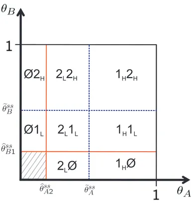
In particular, it is easy to see that the location of indifferent consumers is inde-pendent of the distribution of consumers on the other market. Figure 1 visualizes the demand pattern under the separate pricing regime. Therein, and in all fol-lowing visualizations of demand patterns, I make the convention to denote each distinct demand area by two numbers. The first number specifies the firm and service quality (subscript H for high-quality or subscriptL for low quality) that consumers located in this area will buy in marketA. Likewise, the second number relates to the firm and service quality bought from the same consumers in market B. If a set of consumers buys nothing in marketA(B), then this is denoted by the first (second) number being∅.

1 Ø

1 2

1 1

2 1

2 2

2 Ø

Ø1

Ø2

Figure 1:Demand Pattern under the Separate Pricing Regime

The absence of cross-market effects allows to consider each market separately.

In each market the revenue for the incumbentk (high-quality) and entrantj (low-quality) firm is

Rss

k = 100 (1−θess_m) pss_mk

Rss

j = 100 (θess_m −bθss_m) pss_mj

(2)

Solving for optimal prices and substituting this into the profit functions yields:21

Πss

k = 400 q2

H(qH−qL)

(4qH−qL)2 − c q

e H,

Πss

j = 100

qHqL(qH−qL)

(4qH−qL)2 − c q

e L.

(3)

Obviously, in order for the high-quality advantage principle to hold I must find a constraint onΠss

k >Πssj , which by settingµ= qL

qH rewrites to

c q_He−1(1−µe)<300(1−µ) 2

(4−µ)2. (4)

To be able to compare this result with others obtained later, I will approximate the right hand side of this inequality linearly in the feasible range of µ ∈ (0,1₄]. To this extend, set f(µ) = 300(1₍₄−₋µ_µ)₎22 and notice that

∂f

∂µ < 0. Furthermore f(0) =

18.75and f(1₄) = 12. Thus, the feasibility constraint function, f may be well approximated from above by f(µ) ≈ f(0)−4 f(0)−f(1₄)µ = 18.75−27µ and the Lemma obtains.

First, see thatC = C(qH)

qH (1−µ

e_{), which will be in the center of my analysis,}

is the cost (of quality improvement) measured in units of high-quality times the factor(1−µe)∈(3₄,1). Obviously, the higher thisC, the costlier it is for firms to improve their quality. Thus,C is a measure of how prevalent cost considerations are in the firms’ quality decision process. Moreover, notice that C(qH)

qH = c q

e−1

H ,

whereq_He−1 may be seen as a convexity measure of the cost function and cas the general magnitude of costs. For low values ofC, costs rise only slowly with qual-ity because either convexqual-ity is mild or costs are generally small, or both. Thus, firms will be able to operate profitably here and high-quality providers generally earn more than their low-quality competitors. As C increases, cost considera-tions become increasingly prevalent, until eventually costs are so dominant that the high-quality advantage principle fails to hold and no firm finds it profitable to continue business.

Consequently, for what follows, it makes sense to cut off the unfeasibly high val-ues ofC at the bound identified by Lemma 1.

Proposition 2(Equilibrium and Revenue under Separate Pricing). Under the sep-arate pricing regime, each firms offers a high-quality service in its home market and a low-quality service in its secondary market. Total revenue is approximated by

Rss_i ≈qH (25−

28 3 µ)

Proof. The first part follows directly from my assumptions. From the proof of Lemma 1 we know that the exact revenue function is given byRss

i =qH100(1

−µ)(4+µ) (4−µ)2 . For later comparison, I employ the linear approximation scheme again withRss

i (0) =

25andRss i (

1

4) = 22 2 3.

2.3

Bundle Pricing Regimes

In contrast to the separate pricing regime, which did not evoke any cross-market effects, bundle pricing creates externality on the other market because both bun-dles compete for the same customers. Although consumers tastes for quality are uncorrelated such that there is demand in every ’niche’ of the market, we will see that this externality acts as a quality-sorting mechanism for almost all feasible settings. To fix ideas, set firm1as the high- and firm2as the low-quality provider in marketA. This assumption is without loss of generality, because by the qual-ity differentiation principle in equilibrium firms will differentiate their bundles by choosing a different service quality for at least one service type. Then, my main result is that the high-quality incumbent of marketAcan leverage his qual-ity dominance over to the secondary market, B, thus providing the high-quality product forboth markets and earning greater profits than under separate pricing. This result is robust for all feasible model parameters.

Keeping quality assignments fixed for marketA, it is now at the core of this paper to investigate the quality choice of firms in market B when firm one has chosen a bundle pricing strategy. Certainly, if bundling had no effect on the firms’ quality decision, firm 1(2) would choose qL (qH) in equilibrium again. Denote

this scenario byLH. However, if bundling will indeed serve as a quality sorting mechanism, then firm1should be able to establish itself as the high-quality seller in market B, possibly even forcing the other firm into providing the low-quality service in both markets (scenarioHL). On the other hand, if firm 2choseqH in

1

2

2

LL LH HH HL

qH

qL

qH

qL

1 2

LL LH HH HL

qH

qL

qH

qL

1 2

LL LH HH HL

qH

qL

qH

qL

1 2

LH

s

s

b

s

b

b

ss

sb sb

bs

bs bs

bs bb bb

bb bb

bb

separate pricing

regime bundle pricing regimes

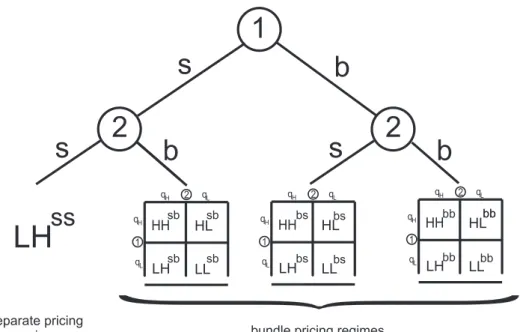
Figure 2:Stylized Game Tree under Sequential Pricing-Strategy Decisions

fix its pricing strategy as well. Then either one of the four pricing regimes (ss, sb, bs orbb) emerges, yielding a normal form game determining the quality decision in market B (cf. Table 1). Moreover, recall that each scenario of each bundle

1\2 qH qL

qH Π1(HH), Π2(HH) Π1(HL), Π2(HL)

qL Π1(LH), Π2(LH) Π1(LL), Π2(LL)

Table 1: Bundle Pricing Subgame: Quality Decisions in MarketB

pricing subgame implies an underlying Betrand price game. Thus in total I have to investigate twelve Betrand price subgames in addition to the separate pricing regime. This is a very tedious and cumbersome task and for readability I have abandoned parts of the proof to the appendix. Within the following subsections, I will consider each bundle pricing subgame separately.

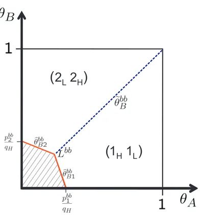
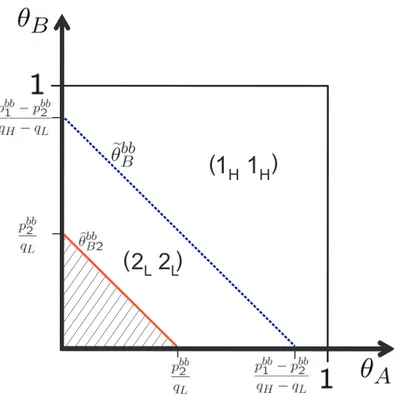
2.3.1 Bundle vs. Bundle Pricing Regime

regimes w.l.o.g. in order to avoid duplicism. Of course all results also hold for the symmetric case where firm 2 would be the designated high-quality firm in market B. The consumers indifferent between firm 1’s and 2’s bundle lie on the line

e

θbb_B = p

bb

1 −pbb2

qB1−qB2

−θA

qH −qL

qB1−qB2

,

wherepbb

i denotes the price of firmi’s bundle. The consumers indifferent between

buying bundle 1 or 2 at all are located along

b

θ_Bbb₁ =p

bb

1

qB1

−θA

qH

qB1

and

b

θ_Bbb₂ =p

bb

2

qB2

−θA

qL

qB2

,

respectively. The locus of consumers indifferent between all three choices (if existent) isLbb_{= (L}bb

A, LbbB), with

Lbb_A =p

bb

1 qB2 − pbb2 qB1

qH qB2 −qLqB1

and

Lbb_B =p

bb

2 qH − pbb1 qL

qH qB2 −qLqB1

.

Notice that the indifferent consumers are now determined by their tastes forboth

service types. These cross-market effects are responsible for the existence of the quality leverage effect.

Next, I will try to give some intuition for the price competition evolving in each of the scenarios. I will employ the visualizations of the demand patterns here to undermine my analysis. The quantitative results are summarized by the subsequent lemmas whose proofs may be found in the appendix.

1

1

2

2

(

(

)

)

Figure 3:Bundle Pricing Subgame: ScenarioLHbb

However, due to symmetry, in equilibrium both firms must offer the same price for their bundles and will consequently earn the same profits. The consumers being indifferent between both service bundles are thus located along the angle bisecting line. Furthermore, the lack of differentiation in the vertical dimension will keep prices and consequently revenues rather low.

1

1

2

2

(

(

)

)

Figure 4:Bundle Pricing Subgame: ScenarioHLbb

ScenariosHHbb _andLLbb_{: Finally, I must consider the case where firms do}

not differentiate their products in market B. Say both firms provide a service of quality qX ∈ {qH, qL} in B. The corresponding demand pattern is given by

Figure 5. In this scenario, the consumers indifferent between both scenarios are all characterized by the same taste for quality in market A, because firms fail to differentiate their services in market B. Price competition is at an intermediate level and largely determined the by the degree of differentiation in market A. Of course, due to the high-quality advantage principle, scenario HH generates higher revenues than scenarioLL. However, for price equilibria to exist in these scenarios, at least firms’ services in marketAmust be sufficiently differentiated.

Lemma 3 shows that the existence of interior price equilibria for these four scenarios generally requires a minimum amount of service differentiation.

Lemma 3 (Price Equilibrium Feasibility Constraints: Pure Bundling). Interior price equilibria exist only if quality levels are sufficiently differentiated. Scenario HLbb _{is feasible forq}

H > 1.77qL, scenarioHHbbforqH > 2.31qL, scenario

LHbb_forq

H > qLand scenarioLLbbforqH > 3.73qL.

Proof. See Appendix.

as-1

1

2_L2_X

(

)

( )

Figure 5:Bundle Pricing Subgame: ScenariosHHbb_andLLbb

sumption, because it ensures the existence of all four scenarios of thebb subgame. AsqLapproachesqH further, the equilibria where both firms provide the same

ser-vice quality in marketB gradually cease to exist. This is intuitively clear, since services must be sufficiently differentiated in marketAif firms fail to distinguish their services in market B. ScenariosHLbb _andLHbb_{, on the contrary, continue}

to hold under significantly less service differentiation. Also keep in mind that the conditions in Lemma 3 are only necessary, because quality levels are exoge-nous. If firms would choose quality levels freely, the classical literature on vertical differentiation has shown that sufficient differentiation arises endogenously, such that interior price equilibria generally exist.

Now, let us turn to a more quantitative analysis of thebb-subgame.

Lemma 4(Revenues in thebb-subgame). The revenue of firmiin each scenario of thebb-subgame, denoted byRbb_i , can be well approximated by

Rbb₁ (HH) =qH(36.88−28µ) , Rbb2 (HH) =qH(6.71−1.54µ)

Rbb₁ (HL) =qH(54.41−29.06µ) , Rbb2 (HL) =qH 8.62µ

Rbb

i (LH) =qH(17.16−3.84µ)

Rbb

Proof. See Appendix.

In particular notice that firms’ revenue depends onqH andqL=µ qH only and

generally increases with quality. In order to determine the quality equilibrium of the bundle pricing regime subgames, I must now define a functionBRi(qj), which

returns firmi’s best quality response, given the quality decision of her opponent, j. The pure quality Nash-equilibrium of each subgame is then given as the steady state characterized byBRi(BRj) = BRi,∀i6=j, from which neither firm wishes

to deviate.

Lemma 5(Best Quality Responses in thebb-subgame). In thebb-subgame, each firms best quality response functionBRbb

i is

BRbb

1 (qL) = (

qH, if C ≤rbb1 (qL) = 29.41−27.56µ

qL, otherwise

BRbb

1 (qH) = (

qH, if C ≤rbb1 (qH) = 19.72−24.16µ

qL, otherwise

BRbb

2 (qL) = (

qH, if C ≤rbb2 (qL) = 17.16−18.37µ

qL, otherwise

BRbb₂ (qH) = (

qH, if C ≤rbb2 (qH) = 6.71−10.16µ

qL, otherwise

For allµ∈ (0,1₄]it holds that the threshold functions, r, can be uniquely ranked asrbb₂ (qH)< rbb2 (qL)< rbb1(qH)< rbb1 (qL).

Proof. The best response function determines whether it is best to reply with a high- or low quality service, given the quality level of the opponents’ service. Consider firm 1, for example. If firm2offers a service of qualityqX ∈ {qH, qL}in

marketB, firm 1 will respond with a high-quality service iffΠ1(HX)≥Π1(LX). Rearranging this inequality yields

c(q_He −q_Le)≤R1(HX)−R1(LX)

Moreover, we know from Lemma 4 that the revenue functions follow the basic form of Ri = qH gi(µ), such that a division by qH together with substituting

qL=µ qH yields

c q_He−1(1−µe)≤r1,

where the left hand side isC = C(qH)

qH (1−µ

e_{)and the right hand side corresponds}

to the threshold functionr1 = R1(HX)

−R1(LX)

Lemma 4 has two important implications. First, notice that the threshold func-tions may be uniquely ranked in terms of C, independent of µ and e. Conse-quently, the Nash-equilibrium of the bb-subgame depends only on the size of the cost prevalence measure, C, and not on the precise relationship betweenqH and

qL. This gives rise to the following Corollary.

Corollary 6 (Independence of Quality Levels). The pure strategy equilibrium of thebb-subgame depends on the cost function only and is independent of whether quality levels are exogenous or endogenously chosen.

Consequently, I obtain qualitatively identical results, although I have simpli-fied the analysis by fixing the quality levels exogenously. Moreover, notice that the feasibility constraint function identified by Lemma 1,f, satisfies

r2(qH)< f < r1(qH)< r1(qL), ∀µ∈(0,

1 4]

which means that the range of feasible C-values is cut-off at a level below the threshold functions,r1, of firm1. The next Proposition follows immediately.

Proposition 7(Equilibria of thebb-subgame and High-Quality Commitment). For all feasible values ofC, firm one choosesqH in marketB as adominant strategy

in thebb-subgame.

Consequently, if costs of quality improvement are negligible (C ≤ rbb

2 (qH))

both firms will provide a high-quality service in marketB (scenarioHHbb). Oth-erwise, if costs of quality improvement are non negligible, the quality sorting effect of bundling forces firms to specialize on providing either a low- or high service quality inbothmarkets (scenarioHLbb).

The first part of Proposition 7 refers to thehigh-quality commitment effect of bundle pricing. Providing a high-quality service in marketB is a credible strategy for the high-quality provider in market A irrespective of the precise fixed cost function. This shows very impressively how powerful the bundle pricing strategy may act as a quality leverage device. To see the second part of the Corollary, let us consider all feasible settings of C in turn. At very small values, i.eC < rbb₂(qH), theHHbbscenario is the unique equilibrium. Here costs have only small

impact on the quality decision and thus both firms strive toward offering a high-quality service. WhenC increases, such thatrbb₂ (qH)< C <min{rbb2(qL), f},22

cost considerations become more prominent, such that scenarioHLis the robust unique equilibrium outcome of the bundle pricing bb-subgame for all remaining settings. Certainly, if rbb₂(qH) < C < rbb2(qL), firm 2 will reply with a

low-quality of service in marketB, should firm1offer a high-quality service (scenario

22_{Precisely,min{r}bb

HLbb) and offer a high-quality service if firm 1 provides a low-quality service (scenario LHbb_{). However, since firm 1 will offer a high-quality service as a}

dominant strategy,HLbb_{is the unique equilibrium scenario here. Likewise, should}

rbb₂(qL) < C < f hold, firm 2 will provide low-quality of service in market B

irrespective of firm 1’s quality choice. That is, in this parameter range firm 1’s high-quality commitment effect is coupled with alow-quality commitment effect

of firm 2. Consequently scenario HLbb emerges as the unique equilibrium in dominant strategies here.

2.3.2 Bundle vs. Separate Pricing Subgame

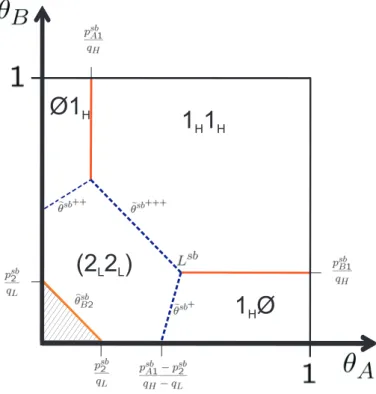
In order to show that the strong results obtained under a bundle vs bundle pricing regime extend to hybrid pricing regimes, I consider the bundle vs. separate pricing subgame next. Here firm one has chosen a bundle pricing strategy, whereas firm 2 seeks to counteract the leverage efforts of firm1by selling its services separately. Since the course of proofs is analogous to the bb-subgame, I will keep the anal-ysis as concise as possible.23 All variables of this subgame will be denoted by a superscriptbs to indicate thebundle vs. separate pricing regime.

In this subgame consumers have the choice of five different service portfolios: They may buy firm 1’s bundle, firm 2’s services separately (either one or both) or refrain from purchasing any service. I must therefore distinguish the following indifferent consumers:24

Consumers indifferent between buying firm1’s bundle and firm2’sA-service sat-isfy

e

θbs_B+ = p

bs

1 −pbsA2

qB1

−θA

qH −qL

qB1

Consumers indifferent between buying firm1’s bundle and firm2’sB-service only are located at

e

θ_Bbs++ = p

bs

1 −pbsB2

qB1−qB2

−θA

qH

qB1−qB2

Consumers indifferent between buying firm 1’s bundle and each of firm 2’s ser-vices separately lie along

e

θbs_B+++ = p

bs

1 −pbsA2−pbsB2

qB1−qB2

−θA

qH −qL

qB1−qB2

Finally, the locus of consumers indifferent between buying firm 1’s bundle and either firm 2’s A-service or both services of firm 2, i.e. whereθebs

+

B = θebs

+++

B is

23_{Of course, details are available in the appendix.}

24_{Not all of these indifferent consumers may be of importance in all of the subsequent scenarios.}

given byLbs = (Lbs_A, Lbs_B), where

Lbs_A = qB2(p

bs

1 −pbsA2) − qB1pbsB2 (qH −qL)qB2

, Lbs_B = p

bs B2

qB2

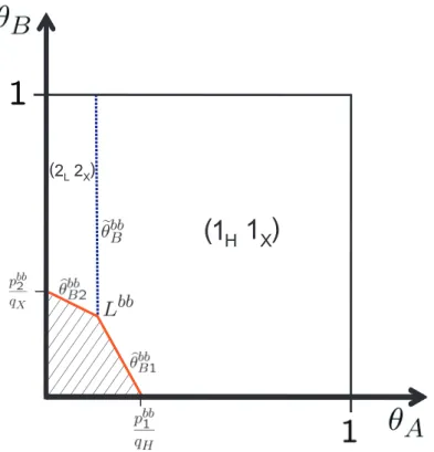
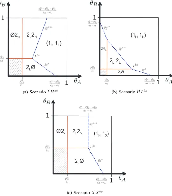
Figure 6 shows the demand patterns for each of the scenarios of thebs-subgame.

1_H1_L

( )

Ø2H

2 ØL

2 2L H

(a) ScenarioLHbs

1_H1_H

2_L2_L

( )

Ø2L

2 ØL

(b) ScenarioHLbs

1_H1_X

( ) Ø2x

2 Ø_L 2 2_{L X}

(c) ScenarioXXbs

Figure 6:Bundle Pricing Subgame: (a) ScenarioLHbs, (b) ScenarioHLbs(c) Scenarios

HHbsandLLbs

This time theLHbs scenario is not perfectly symmetric because the firms employ different pricing strategies. Although both firms offer a high-quality service in their home market and a low-quality service in their secondary market, the use of different pricing strategies creates some artificial differentiation between the firms’ service portfolios. Hence, we may already conclude from Figure 6(a) that price competition is less intense than underLHbb_{. However, by offering its}

ser-vices separately, firm 2 induces some self-inflicted competition among its own services. We may thus conjecture that firm2’s revenues are lower underLHbs _as

compared withLHbb_{. Consequently, counteracting firm1’s bundling strategy by}

a separate selling strategy may not be firm2’s best choice when it simultaneously tries to prevail its high-quality leadership in marketB.

Next, consider scenario HLbs_{. Figure 6(b) shows that although firm 1’s bundle}

competes against more distinct service portfolios, the nature of competition is very similar to that fromHLbs_{: Firm1serves the high-quality consumer segment,}

whereas firm 2 offers low-quality services. By offering its services separately, firm 2induces some self-inflicted competition again, however, on the other side it also seems to capture some more consumers by doing so (especially those with extreme differences in θ across markets). In summary, we can expect revenues akin to those inHLbb.

Similar holds for the scenariosXXbs_{, where firms offer the same service quality}

in market B. Again, firm 1is able to attract the most valuable consumers with high θ values in both markets and will therefore achieve higher revenues. By its separate pricing strategy, firm 2 is able to steal some demand in the low θB

segment, but also suffers from self-inflicted competition again.

The corresponding quantitative analysis may be found in the appendix and is summarized by the following lemmas.

Lemma 8(Revenues in thebs-subgame). The revenue of firmiin each scenario of thebs-subgame can be well approximated by

Rbs

1 (HH) =qH(36.9−30.56µ) , Rbs2 (HH) = qH(6.71−3.28µ)

Rbs

1 (HL) =qH(54.41−31.36µ) , Rbs2 (HL) =qH 6.65µ

Rbs

1 (LH) =qH(35.09−27µ) , R2bs(LH) =qH(5.88−1.69µ)

Rbs

1 (LL) =qH(25−0.95µ) , Rbs2 (LL) =qH 13.47µ

Proof. See Appendix.

firm’s best quality response function is

BRbs₁ (qL) = (

qH, if C ≤rbs1 (qL) = 29.41−30.41µ

qL, otherwise

BRbs

1 (qH) = (

qH, if C ≤rbs1 (qH) = 1.81−3.56µ

qL, otherwise

BRbs

2 (qL) = (

qH, if C ≤rbs2 (qL) = 5.88−15.16µ

qL, otherwise

BRbs

2 (qH) = (

qH, if C ≤rbs2 (qH) = 6.71−9.93µ

qL, otherwise

For allµ∈ (0,1₄]it holds that the threshold functions, r, can be uniquely ranked asrbs₁ (qH)< rbs2 (qL)< rbs2 (qH)< f < rbs1 (qL).

Proof. Analogous to Lemma 5

Lemma 9 reveals two major differences of thesb-subgame compared to the bb-subgame. First, due to the asymmetry and resulting weak price competition in scenario LHbs, firm1 is able to achieve much higher revenues here. Conse-quently, LHbs _{is much more appealing to firm 1 and BR}bs

1 (qH) = qL at small

C values already. Likewise, compared to LHbb_{, firm2 is worse off in scenario}

LHbs, which in turn raises the attractiveness of scenarioLLbs for firm 2. There-foreBRbs

2 (qL) =qLholds for much lower values ofC than before. The remaining

best response functions have changed only little in comparison to thebb-subgame. Second, the diminishing revenue differences across neighboring scenarios also disposes firm1’s high quality commitment effect. In fact, firm1is the first to give into providing a low-quality of service in marketB, onceC > rbs₁ (qH), such that

scenarioLHbs obtains as the equilibrium of thebs-subgame here. If cost considerations become more prominent, i.e. C > rbs

2 (qL), scenarioHLbs

is the unique equilibrium of thesb-subgame again. To see this considerrbs₂ (qH)>

C > rbs₂ (qL)first. Here scenario LHbs cannot be sustained in equilibrium

any-more, because firm 2 wishes to deviate into LLbs_{. Given q}

B2 = qL, however,

firm 1 would choose BRbs

1 (qL) = qH in market B. When costs rise further to

f > C > rbs₂ (qH), firm 2’s low-quality commitment effect is viable again and

firm1will respond with a high-quality service sinceBRbs

1 (qL) =qH. This proofs

the following Proposition.

If costs of quality improvement are negligible firms will either both provide a high-quality service in market B (scenario HHbs_{) when C ≤ r}bs

1 (qH) or offer

a high-quality service in their home market and a low-quality service in their secondary market (scenarioLHbs), ifrbs₁ (qH)<C ≤rbs2 (qL).

2.3.3 Separate vs. Bundle Pricing Regime

The separate vs. bundle pricing regime (sb-subgame) obtains when firm1chooses a separate pricing strategy and firm2a bundle pricing strategy.

Lemma 11 (Revenues in the sb-subgame). Revenues in the bs-subgame can be well approximated by

Rsb₁ (HH) = qH(25−11.32µ) , Rsb2 (HH) =qH(8µ)

Rsb

1 (HL) =qH(50.72−27.43µ) , Rsb2 (HL) =qH 6.09µ

Rsb

2 (LH) =qH(5.88−1.69µ) , Rsb2 (LH) =qH(35.09−27µ)

Rsb

1 (LL) =qH(25−13.58µ) , Rbs2 (LL) =qH 7.26µ

Proof. First notice that scenarioLHsb _{is identical to scenarioLH}bs_{, just with the}

role of each firm interchanged. Thus, equilibrium revenues can be derived from Lemma 8 and by interchanging firms’ indices. The rest of the proof may be found in the appendix.

Furthermore, best responses are given by:

Lemma 12(Best Quality Responses in thesb-subgame). In thesb-subgame, each firm’s best quality response function is

BRsb₁ (qL) = (

qH, if C ≤rsb1 (qL) = 25.72−13.85µ

qL, otherwise

BRsb

1 (qH) = (

qH, if C ≤rsb1 (qH) = 19.12−9.63µ

qL, otherwise

BRsb

2 (qL) = (

qH, if C ≤rsb2 (qL) = 35.09−34.26µ

qL, otherwise

BRsb

2 (qH) = (

qH, if C ≤rsb2 (qH) = 1.91µ

qL, otherwise

For allµ∈ (0,1₄]it holds that the threshold functions, r, can be uniquely ranked asrsb

2 (qH)< rsb1 (qH)< rsb1 (qL)< rsb2 (qL).

The next proposition then follows immediately.

Proposition 13 (Equilibria of thesb-subgame). If costs of quality improvement are non negligible (in the sense of Proposition 7), either scenario HLsb _or

sce-narioLHsbwill obtain.

If costs of quality improvement are negligible, eitherHHsb_{is the unique}

equi-librium scenario whenC ≤rsb

2 (qH), or otherwise scenarioHLsbobtains.

2.4

Equilibrium Pricing Strategies and Leverage

Before I proceed to determine firms’ equilibrium pricing strategies in the first stage of the game, two general statements concerning the second stage shall be pointed out.

First, notice that Propositions 7 and 10 show that bundle pricing indeed serves as a quality leverage device for all settings were costs are relevant. If firm1commits to a bundle pricing strategy in stage one, scenarioHLobtains, which–due to the high-quality advantage effect–is more profitable to firm 1 than the separate pricing regime or any otherLH scenario.

Second, subgamesbseems not to be very tempting for firm1, sinceRsb

1 (XY)≤

Rbb

1(XY),∀µ ∈ (0,14], where X, Y ∈ {H, L}. In particular, this means that

the bb-subgame is ex-post credible because firm 1 would never wish to deviate into the sb- subgame, once the quality decision has been fixed.25 _{This is}

impor-tant, because in my model, I show that the pricing strategy (which includes little commitment) has influence upon the firms’ quality decision (which requires sunk investments and thus high commitment). Hence, if firm1can force firm 2 into the bb-subgame, and influence it to provide a low-quality service through the quality sorting mechanism of bundling, then ex-post credibility ensures that firm 1 has no incentive to deviate from its pricing strategy, once the beneficial quality config-uration has been obtained.26 _{Consequently, contrary to Whinston (1990), in my}

model firm 1 does not need any exogenous commitment to bundling in order to achieve market leverage. Bundle pricing remains an equilibrium strategy, even after it has altered the nature of competition in the market.

2.4.1 Non Negligible Costs

Consider the case of non negligible costs of quality improvement first, i.e C > rbb

2(qH). From the subgame equilibrium propositions 10 and 7, I can directly

25_{It is easy to see that similar holds for a deviation from thebs-subgame to the separate pricing}

regime (ss).

26_{Since firm2is the second-mover it will always choose the optimal pricing strategy in response}

conclude that scenarioHLwill obtain whenever firm1chooses bundling in stage one. In this case, firm 2 comparesR2(HLbb) > R2(HLbs), and is consequently

best off by responding with a bundle pricing strategy itself. The next lemma follows:

Lemma 14(Equilibrium under Non Negligible Costs). For firm1it is a dominant strategy to choose bundle pricing if costs of quality improvement are non negligi-ble. Firm2will respond by bundle pricing itself and scenarioHLbbobtains as the unique equilibrium of the game.

Proof. The second part of the lemma has been shown above. If firm1chooses a separate pricing strategy in the first stage of the game, by Propositions 2 and 13 either scenario HLsb_{, LH}sb _{or LH}ss _{will obtain. Thus,it remains to verify that}

Π1(HLbb) > max{Π1(HLsb),Π1(LHsb),Πss1 }. Π1(HLbb) > Π1(HLsb)follows

trivially from Lemmas 4 and 11. Next, from Proposition 2 and Lemma 11, we can directly conclude that Π1(LHsb) > Πss1 . Finally, it holds that Π1(HLbb) > Π1(LHsb) iff 48.53−27.37µ > C > f, i.e for all feasible parameter values.

Taken together, this proofs the lemma.

2.4.2 Negligible Costs

First see that if costs of quality improvement are negligible, subgame sb is not very appealing to firm2. This is because forC < rbb₂ (qH), either HHbs orHLbs

obtain, which both yield lower profits for firm2than if it would have opted out for the separate pricing regimeLHss_.27 _{Thus, should firm1choose a separate pricing}

strategy, firm 2 will counteract by pricing its services separately as well and the separate pricing regimessobtains. The next lemma shows that firm2’s tendency to mirror firm1’s pricing strategy holds more generally.

Lemma 15(Equilibrium under Negligible Costs). Under negligible costs, firm2

always seeks to choose the same pricing strategy as firm 1. Thereby, scenario HHbb_{emerges as the unique equilibrium of the game.}

Proof. Consider the first part of the lemma. We have already seen that separate pricing is firm 2’s best response to a separate pricing strategy by firm 1. If firm

1chooses a bundle pricing strategy, I must consider three different cases:(i) C ≤

rbs₁ (qH): Here, firm 2 compares Π2(HHbb) > Π2(HHbs) and chooses bundle

pricing. (ii) rbs₁ (qH) < C ≤ rbs2 (qL): This time Π2(HHbb) > Π2(LHbs) and

firm 2chooses bundle pricing again. (iii) rbs

2 (qL) < C ≤ rbb2(qH): Now firm2

compares Π2(HHbb) > Π2(HLbs), which holds for all C < f. Thus, bundle

27_WhereasΠ

pricing is firm2’s best response to bundle pricing by firm1.

For the second part of the lemma, I must thus compare Π1(HHbb) > Πss1 . This

inequality rewrites to29.41−19.73µ > f >C and the lemma obtains.

2.5

Quality Leverage through Bundling

The previous analysis has revealed two major findings. First, firms have a ten-dency to symmetric pricing, i.e. either both firms employ separate- or bundle pricing. This justifies to focus future attention on the separate pricing and all bundle pricing regime (subgamebb). Second, the all bundle pricing regime is the robust equilibrium-subgame under all feasible model parameters.

If costs of of quality improvement are non negligible scenario HLbb _constitutes

the unique equilibrium of the game. The HLbb _{scenario is so appealing to the}

firms because it allows them to affectively shield themselves from the aggressive Bertrand price competition by segmenting the market into low- and high-quality buyers. By the high-quality advantage, in scenarioHLbb_{firm1is much better and}

firm2worse off than under the separate pricing regime. Conversely, if under the all bundle pricing regime firms would have continued to provide a high-quality service in their home market and a low-quality service in their secondary market (LHbb scenario), price competition would have intensified compared to the sep-arate pricing strategy because bundles became relatively close substitutes. Thus, both firms would rather price their products separately than choosingLHbb_under

a bundle pricing strategy.

If costs considerations become negligible, scenario HHbb _{obtains. In fact, costs}

are so small that firm1cannot prevent firm2from participating of the high-quality advantage itself, which is in turn so large that it even recoups the losses incurred from intensified price competition. This eventually leads to higher profits than under separate pricing.

Thus, under all settings firm 1 can achieve market leverage by choosing a bundle pricing strategy in the first stage of the game. We have seen that this leverage effect is achieved through aquality leveragemechanism which relates to increased profits due to the high-quality advantage principle. In particular, notice that bundle pricing is anex-post credibleequilibrium strategy and requires no ex-ante commitment of the first-mover. Moreover, if costs are non negligible this outcome is invariant with respect to simultaneous or sequential moves in stage one, because then bundle pricing is firm1’s dominant strategy. Eventually, this is summarized by my main proposition.

separate pricing regime.

3

Welfare Effects

To round off the analysis, let us briefly consider the welfare effects induced by the transition from the separate pricing to the bundling regime. As usual welfare is given by the sum of consumers’ and producers’ surplus. For conciseness I will only compare the welfare differences between separate pricing and theHLbb scenario.

Consider producers’ welfare first and recall that by Proposition 2 firms earn equal profits under separate pricing as they both provide a high- and a low-quality service. With bundle pricing, however, firms specialize on serving either the low-or high-quality end of the market (scenarioHLbb_{), leading to an increase of firm}

1’s profit at the expense of firm2’s, compared to the profits under separate pricing. Thus, ex-ante it is not clear whether producers’ surplus is raised or lowered in the transition. Obviously, since in both scenarios the same service qualities are offered in the economy, just by different providers, cost differences cannot account for a prospective change in producers’ surplus. Therefore, the results obtained here are not peculiar to the specifics of the cost function.

Lemma 17 (Producers’ Surplus under Bundling). Producers’ surplus is higher under the bundle pricing regime (HLbb_{scenario) than under the separate pricing}

regime.

Proof. Since overall costs are identical underHLbband the separate pricing regime, I must show merely that

∆P S_bbss(HL) =R₁bb(HL) +Rbb₂(HL)−2(Rss_h +R_lss)>0 (5)

In particular, by Proposition 2 and Lemma 4, I can directly conclude that∆P Sss bb(HL)

≈qH(4.41−1.77µ)>0forµ∈(0,1₄].

Therefore, although firm 2 is worse off under HLbb_{, the quality sorting}

ef-fect of bundling mitigates competition such that overall producers’ surplus is in-creased. However, when taking a course of action, regulators are usually more concerned with consumers’ surplus or at least total welfare. More precisely, whether consumers’ surplus is increased or decreased hinges upon the direction and size of the price and the bundling effect. In the present setting, the price effect is positive, because the prices for the low- and high-quality bundle are smaller underHLbb _{than their corresponding counterparts under individual pricing}

Figure 7: Positive Price Effect: Prices of the low- (solid line) and high-quality bundle (dashed line) in per cent of the price for the corresponding service package under separate pricing.

notion of a bundle discount, the economic interpretation must moreover explain why firms’ profits can rise (Lemma 17) while prices drop. Both can be attributed to thebundling effect.

On the one hand, selling bundles leaves consumers with less options: Under sep-arate pricing each consumer can compile his optimal service package, possibly consisting of low- and high-quality services from different firms. In total, con-sumers can choose between nine different service combinations, including the no buy option. Under the bundle pricing regime, however, consumers have only three options left–to buy the service package of either firm, or not to buy anything at all. As a consequence, many consumers are forced into buying a high-quality service bundle they would not have purchased before. In this way the bundling effect negatively influences consumers’ welfare, but increases producers’ surplus, of course.

On the other hand, the consumers’ lack of choice is also a lack of differentiation on the providers’ side. Whereas under the separate pricing regime a small change in price would induce consumers to switch their provider for only one service type, a similar price might provoke consumers to change their provider altogether under the bundle pricing regime. Thus, bundling evokes an all-or-nothing effect which leads to increased price competition and thereby lower prices.28

Lemma 17 has confirmed that the bundle effect outweighs the price effect for the providers. Conversely, lemma 18 reveals that for the consumers, the price effect offsets the welfare losses incurred by the bundle effect.

Lemma 18(Consumers’ Surplus under Bundling). Consumers’ surplus is higher under the bundle pricing regime (HLbb_{scenario) than under the separate pricing}

regime.

Proof. See Appendix

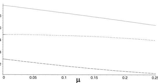
Figure 8: Absolute difference of consumers’ (dashed line), producers’ (dotted line) and total welfare (solid line) between the bundling and the separate pricing regime in units of

qH.

The next proposition then follows trivially.

Proposition 19. Total welfare is higher under the bundle pricing regime (HLbb

scenario) than under the separate pricing regime.

4

Conclusion

The previous analysis was based on a reciprocal duopoly setting with home mar-kets, which is believed to have been constituted through digital convergence of communication and entertainment media services. In practice, these services are

Recall that among the scenarios of the bundle pricing regimes, prices are among the highest in the

offered by former telecommunication and cable monopolists which sell them in a bundle—the so-calledTriple Play package. I have investigated whether bundling of services is indeed a profitable pricing strategy, if it can facilitate market power leverage and if it emerges as an equilibrium strategy. To this extend, a three-stage game was considered, where in stage one firms decide whether to offer services in a bundle or separate and in stage two and three decide upon quality and price, respectively. I could show that bundling serves as a powerful leverage device in this industry. This is achieved through a quality sorting effect accruing as the firms wish to shield themselves from increased price competition in the market for bundles. Thereby, one firm emerges as the high-quality, high-profit provider in both markets, whereas the competing firm has to settle for low qualities and profits. The leverage effect is said to be ’powerful’ because it holds under a num-ber of worst-case assumptions. First, recall that market power is rather limited in the present framework because neither firm holds a monopoly position. Nev-ertheless, leverage is achieved under all feasible settings. Next, I have restricted the analysis to those settings for which price equilibria exist for all four possible scenarios of the bundling subgame. As I have argued, alternative settings tend to strengthen my results. Finally, I have assumed consumers’ ’taste’ for quality to be uncorrelated across service types. This, of course, is least appreciated by the quality sorting mechanism because demand is evenly spread out up to every corner of the market. If rather consumers’ taste was positively correlated, price competition under the LH scenario would intensify yet more and thus promote HLas the equilibrium outcome even further.

Furthermore, as firms bundle their products consumer’s and producers’ wel-fare unambiguously rises, because both prices fall and consumers subscribe to more high-quality services. Previous work has either found bundling as detrimen-tal to welfare or, at best, attributed ambiguous welfare effects to it. The present analysis thus provides a counterbalance by showing that regulators should not con-demn bundling per se but should rather judge on a case by case basis, especially accounting for different market structures.

References

Adams, William James, and Janet L. Yellen. Aug., 1976. “Commodity Bundling and the Burden of Monopoly.” The Quarterly Journal of Economics90 (3): 475–498.

Anderson, Simon P., and Luc Leruth. 1993. “Why firms may prefer not to price discriminate via mixed bundling.” International Journal of Industrial Organization11 (1): 49 – 61 (1993/3).

Aoki, Reiko, and Thomas J. Prusa. 1996. “Sequential versus simultaneous choice with endogenous quality.” International Journal of Industrial Organization 15 (1): 103–121 (February).

Bakos, Y., and E. Brynjolfsson. 1999. “Bundling Information Goods: Pricing, Profits, and Efficiency.” Management Sciences45:1613–1630.

. 2000. “Bundling and Competition on the Internet: Aggregation Strate-gies for Information Goods.” Marketing Science19 (1): 63–82.

Boom, Anette. Mar., 1995. “Asymmetric International Minimum Quality Stan-dards and Vertical Differentiation.” The Journal of Industrial Economics43 (1): 101–119.

Bowman, Jr.W.S. 1957. “Tying Arrangements and the Leverage Problem.” Yale

Law Journal67:19–36.

Carbajo, Jose, David de Meza, and Daniel J. Seidmann. Mar., 1990. “A Strategic Motivation for Commodity Bundling.” The Journal of Industrial Economics 38 (3): 283–298.

Carlton, D.W, and M. Waldmann. 2002. “The Strategic Use of Tying to Pre-serve and Create Market Power in Evolving Industries.” RAND Journal of

Economics33:194–220.

Chae, Suchan. 1992. “Bundling subscription TV channels : A case of natural bundling.” International Journal of Industrial Organization 10 (2): 213 – 230 (1992/6).

Chen, Yongmin. Jan., 1997. “Equilibrium Product Bundling.” The Journal of Business70 (1): 85–103.

Choi, Chong Ju, and Hyun Song Shin. Jun., 1992. “A Comment on a Model of Vertical Product Differentiation.” The Journal of Industrial Economics40 (2): 229–231.

Choi, J.P. 2003. “Bundling new products with old to signal quality, with applica-tion to the sequencing of new products.” International Journal of Industrial

. 2004. “Tying and Innovation: A Dynamic Analysis of Tying Arrange-ments.” The Economic Journal114:83–101.

Diallo, Thierno. 2006. “Bundling in Vertically Differentiated Communication Markets.” Universit´e du Qu´ebec `a Chicoutimi.

Director, Aaron, and Edward Levi. 1956. “Law and the Future: Trade Regula-tion.” Northwestern University Law Review51:281–296.

Economides, Nicholas. 1993, November 1993. “Mixed Bundling in Duopoly.” Stern School of Business, New York University.

Economides, Nicholas, and William Lehr. 1995. “The Quality of Complex Sys-tems and Industry Structure.” Edited by William Lehr,Quality and Reliability of Telecommunications Infrastructure. Lawrence Erlbaum, Hillsdale.

Gabszewicz, J., and J.F. Thisse. 1979. “Price Competition, Quality, and Income Disparities.” Journal of Economic Theory20:340–359.

Kopalle, P.K., A. Krishna, and J.L. Assuncao. 1999. “The Role of Market Expansion on Equilibrium Bundling Strategies.” Managerial and Decision

Economics20:365–377.

Lehmann-Grube, Ulrich. Summer, 1997. “Strategic Choice of Quality When Quality is Costly: The Persistence of the High-Quality Advantage.” The

RAND Journal of Economics28 (2): 372–384.

Martin, Stephen. 1999. “Strategic and welfare implications of bundling.” Eco-nomics Letters62 (3): 371 – 376 (1999/3/1).

Matutes, C.; Regibeau, P. 1992. “Compatibility and Bundling of Complementary Goods in a Duopoly.” The Journal of IndustrialEconomics40:37–54.

McAfee, R. Preston, John McMillan, and Michael D. Whinston. May, 1989. “Multiproduct Monopoly, Commodity Bundling, and Correlation of Values.” The Quarterly Journal of Economics104 (2): 371–383.

Moorthy, K.S. 1988. “Product and Price Competition in a Duopoly.” Marketing

Science7:141–168.

Motta, Massimo. Jun., 1993. “Endogenous Quality Choice: Price vs. Quantity Competition.” The Journal of Industrial Economics41 (2): 113–131.

Mussa, Michael, and Sherwin Rosen. 1978. “Monopoly and product quality.” Journal of Economic Theory18 (2): 301–317 (August).

Nalebuff, Barry J. 2004, 01.09.2004. “Bundling as a Way to Leverage Monopoly.” Yale School of Economics.

Posner, R.A. 1976. Antitrust Law: An Economic Perspective. University of Chicago Press.

Reisinger, Markus. 2006, 04.08.2006. “Product Bundling and the Correlation of Valuations in Duopoly.” University of Munich.

Ronnen, Uri. Winter, 1991. “Minimum Quality Standards, Fixed Costs, and Competition.” The RAND Journal of Economics22 (4): 490–504.

Salinger, M.A. 1995. “A Graphic Analysis of Bundling.” Journalof Business 68:85–98.

Schmalensee, Richard. 1982. “Commodity Bundling by a Single-Product Mo-nopolist.” Journal of Law and Economics25:67–71.

. 1984. “Gaussian Demand and Commodity Bundling.” Journal of Busi-ness57:211–230.

Seidmann, Daniel J. Nov., 1991. “Bundling as a Facilitating Device: A Reinter-pretation of Leverage Theory.” Economica58 (232): 491–499.

Selten, Reinhardt. 1975. “Reexamination of the Perfectness Concept for Equi-librium Points in Extensive Games.” International Journal of Game Theory 4:141–201.

Shaked, Avner, and John Sutton. 1982. “Relaxing Price Competition Through Product Differentiation.” The Review of Economic Studies49 (1): 3–13.

. 1983. “Natural Oligopolies.” Econometrica51:1469–1483.

Spector, David. 2007. “Bundling, Tying, and Collusion.” International Journal of Industrial Organization25:575–581.

Tirole, Jean. 1988. The Theory of Industial Organization. MIT Press.

Whinston, Michael D. Sep., 1990. “Tying, Foreclosure, and Exclusion.” The

American Economic Review80 (4): 837–859.

Appendix

A.1

Proof of Lemma 3