Galaxy evolution: A new version of the Besançon Galaxy Model constrained with Tycho data

Galaxy evolution: A new version of the Besançon

Galaxy Model constrained with Tycho data

Maria A. Czekaj

Aquesta tesi doctoral està subjecta a la llicència Reconeixement- NoComercial – SenseObraDerivada 3.0. Espanya de Creative Commons.

Esta tesis doctoral está sujeta a la licencia Reconocimiento - NoComercial – SinObraDerivada 3.0. España de Creative Commons.

This doctoral thesis is licensed under the Creative Commons

Departament d’Astronomia i Meteorologia

Galaxy evolution : A new version of the Besan¸

con

Galaxy Model constrained with Tycho data

Mem`

oria presentada per

Maria A. Czekaj

per optar al grau de

Doctor per la Universitat de Barcelona

Programa de doctorat en F´ısica

Galaxy evolution : A new version of the Besan¸

con

Galaxy Model constrained with Tycho data

Mem`

oria presentada per

Maria A. Czekaj

per optar al grau de

Doctor per la Universitat de Barcelona

Directors de la tesi:

Dra. Annie C. Robin

Dra. Francesca Figueras

First of all I would like to thank to my supervisors Dra. Francesca Figueras, Dra. Annie C. Robin and Dr. Xavier Luri for the knowledge they have passed me, their time and support and for the four fruitful years of our collaboration. Special thanks to Annie for arranging my visits to Besan¸con and for being so hospitable that I could feel like at home. That place has a special energy and will always remain close to me. Special thanks to Francesca for her didactic approach, patience to explain and teach, and for her great support in the last weeks and days before delivering this thesis. And also special thanks to Xavier for helping me with the code development tasks and to manage heavy computations and also for showing me many times that the best solutions are the simplest ones and they can be found with calm.

Thanks to Dr. Jordi Torra, as Scientist in Charge for the Barcelona University in the ELSA Marie Curie Research Training Network, for accepting me as ELSA PhD fellow and giving me this great opportunity of studying in Barcelona.

Big thanks to all the members of the Gaia team and all colleagues at the Univer-sity of Barcelona and as well to my colleagues at the Observatory of Besan¸con.

Special thanks to Dr. Misha Haywood and Dr. Luis Aguilar for their support and for sharing their knowledge and experience with me.

Many thanks to my teachers and professors in Poland for guiding me towards this PhD project, especially to prof. S lawomir Breiter for his support, humor and constant correspondence.

I would also like to thank to my wonderful family for their love and for being so close to me although physically I am always far away. Big thanks to all my friends and especially to Pat for making home with me here in Barcelona.

I dedicate the fruit of my work to people who have dedicated their lives to help other people. For that my very special thanks to maestro Son Kye-Dong, dear Babaji Jose and my Omi. They will probably never read this thesis, but a written word keeps its energy forever, so I would like to thank them for curing my body and inspiring the evolution of my inner self.

I dedicate the following words of Alan Wilson Watts to all my colleagues who at daily basis are struggling with the Universe:

“Through our eyes, the universe is perceiving itself. Through our ears, the uni-verse is listening to its harmonies. We are the witnesses through which the uniuni-verse becomes conscious of its glory, of its magnificence.”

I hope that one day we all will see the universes that are within us.

Uno de los principales objetivos de la misi´on Gaia (ESA, lanzamiento previsto para oto˜no de 2013) es avanzar en el conocimiento del origen y la evoluci´on de nues-tra Galaxia. Para poder realizar una ´optima explotaci´on cient´ıfica de los datos que aportar´a este sat´elite es fundamental disponer de modelos y c´odigos que permitan contrastar varias hip´otesis y escenarios sobre los procesos de formaci´on y evoluci´on de las componentes gal´acticas. Cada una de estas componentes - disco delgado, disco grueso, halo y bulbo - viene caracterizada por una ley de densidad (recuentos estelares) y unas propiedades cinem´aticas. Son tambi´en ingredientes fundamentales del modelo las propiedades de las estrellas, caracterizadas a partir de los modelos de evoluci´on estelar y los modelos de atm´osfera. As´ı tambi´en, un correcto tratamiento de los sistemas binarios en funci´on de los par´ametros f´ısicos estelares es esencial en este tipo de estudios. Todo este conjunto de ingredientes permiten caracterizar las poblaciones estelares a nivel global y, de aqu´ı, inferir la distribuci´on total de masa y el potencial gravitacional gal´actico.

Para abordar este objetivo, en la presente tesis doctoral nos hemos propuesto optimizar el llamado modelo de s´ıntesis de poblaciones estelares de Besan¸con, cuya primera versi´on fue desarrollada por A. Robin en 1986. En particular nos hemos centrado en la componente del disco delgado de la V´ıa L´actea. Cuando iniciamos nuestro trabajo, hace ya cuatro a˜nos, dicho modelo simulaba el contenido estelar en una direcci´on del cielo dado usando los llamados diagramas de Hess. Para una poblaci´on dada, este diagrama estaba fijado, y se calculaba imponiendo, de ante-mano, una funci´on inicial de masa (IMF), una historia de formaci´on estelar (SFR), un modelo de evoluci´on estelar y una relaci´on metalicidad-edad. Ello conllevaba que cualquier generaci´on de un cat´alogo estelar mediante dicha versi´on mantuviese fijos ingredientes tan fundamentales y poco conocidos como son la IMF o la SFR, par´ametros que Gaia deber´a redefinir en la pr´oxima d´ecada.

Esta tesis ofrece una nueva versi´on del modelo de Besan¸con. Hemos dise˜nado, desarrollado, implementado y testeado una nueva estructura de generaci´on de las estrellas del disco delgado, una estructura que permite, mediante la comparaci´on de los datos observados y los generados, encontrar la mejor combinaci´on de IMF y SFR que ajusta a las observaciones. Como se detalla en el cap´ıtulo 2, el c´odigo que pre-sentamos permite imponer la autoconsistencia din´amica en el proceso de generaci´on estelar. Esta se realiza siguiendo los modelos propuestos por Bienayme et al. (1987). Para cada nuevo escenario de evoluci´on (IMF, SFR, modelos de evoluci´on estelar, . . . ) se recalcula el potencial gal´actico y de aqu´ı las leyes de densidad que nos

mitir´an generar un cat´alogo din´amicamente autoconsistente. La segunda aportaci´on importante de esta tesis es la capacidad del nuevo modelo de Besan¸con de generar sistemas binarios. Hasta la fecha, dicho modelo, disponible en la web y de uso li-bre para toda la comunidad internacional, solo permit´ıa la generaci´on de estrellas individuales (Robin et al. 2003). Si bien el simulador de Gaia, cuya descripci´on del contenido estelar ha sido recientemente publicada en Robin et al. (2012), inclu´ıa ya la generaci´on de sistemas binarios, tampoco contemplaba algo tan fundamental como es la autoconsistencia din´amica, es decir la conservaci´on de la masa total observada en el entorno solar. En la versi´on que se presenta en esta tesis doctoral este tema ha sido tratado y testeado con rigor de forma que podemos afirmar que el contenido estelar que genera el nuevo modelo mantiene las restricciones de la densidad local observada, restricciones que se derivan de la funci´on de luminosidad observada en el entorno solar.

Los cap´ıtulos 2 y 3 incluyen una descripci´on detallada de la nueva estructura del c´odigo, de las actualizaciones de todos los ingredientes del modelo de acuerdo con los avances en los ´ultimos diez a˜nos en astrof´ısica gal´actica y evoluci´on estelar, as´ı como de los procesos de generaci´on de sistemas binarios. En el cap´ıtulo 4 discutimos los dos elementos observacionales clave para el ajuste entre modelo y observaci´on: la funci´on de luminosidad observada en el entorno solar y el cat´alogo de Tycho, ambos aportaciones relevantes de la misi´on Hipparcos de la ESA (Perryman et al., 1997). Una vez desarrolladas las herramientas que permiten este ajuste entre modelo y ob-servables (ver cap´ıtulo 4), en el cap´ıtulo 5 pasamos a seleccionar los escenarios de evoluci´on estelar y gal´actica que permiten un mejor ajuste del modelo a los datos observacionales. Dicho cap´ıtulo muestra otro de los logros de la presente tesis doc-toral: por primera vez hemos conseguido un ajuste aceptable a los recuentos estelares y distribuciones de color observados por Hipparcos hasta magnitud visible aparente 11. En este cap´ıtulo mostramos los efectos que resultan de variar cada uno de los ingredientes b´asicos del modelo, desde el cambio de los modelos de atm´osfera o los modelos de evoluci´on estelar al uso de uno u otro modelo de extinci´on interestelar. Tambi´en, como ejemplo, en esta secci´on se han analizado los efectos en los recuentos estelares derivados de imponer una u otra masa din´amica del sistema gal´actico. En conclusi´on, esta tesis nos proporciona una visi´on global no solo de los ingredientes que componen el puzle del disco delgado de nuestra Galaxia sino tambi´en de los efectos que cada uno de estos produce en la componente estelar que observamos en una direcci´on del cielo dada.

The construction of a dynamical model of the Milky Way from the upcoming Gaia data will require a complex comparison between models and data in the space of the observables. To be ready for this challenge, in this PhD thesis, we have optimized the Besan¸con stellar population synthesis model. The new version of the model has been constructed and ingredients as critical as the IMF, the SFR, the binary fraction, the age-metallicity relation and the age-kinematic relation can now be fitted to the observed data. The optimization includes also the use of most updated evolutionary tracks and model atmospheres. Various scenarios for those parameters have been checked against the Tycho-2 data.

Research Training Network ”European Leadership in Space Astrometry” (ELSA) MRTN-CT-2006-033481 of the VIth Framerwork Programm - European Community and the MICINN (Spanish Ministry of Science and Innovation) - FEDER through grant AYA2009-14648-C02-01. This thesis has been carried out at the Department d’Astronomia i Meteorologia (Universitat de Barcelona) and the Observatoire de Besan¸con (France). This study was partially supported by the Gaia Research for European Astronomy Training (GREAT) 08-RNP-118 European Science Foundation (European RNP FP7) and the MICINN - AYA2009-08488-E/AYA.

Contents

1 Introduction 15

2 The Besan¸con Galaxy Model - the code 19

2.1 The Besan¸con Galaxy Model up to now . . . 19

2.2 A new approach to the BGM . . . 26

2.2.1 The overall structure . . . 26

2.2.2 Determination of the mass model . . . 30

2.3 The code and its implementation . . . 38

2.3.1 The thin disc treatment . . . 38

2.3.2 Binarity . . . 45

2.4 New processing modes . . . 46

3 The update of model’s inputs 51 3.1 The Initial Mass Function . . . 51

3.2 The Star Formation Rate . . . 56

3.3 Evolutionary tracks sets . . . 59

3.4 Binarity . . . 63

3.5 Atmosphere models . . . 63

3.6 Age-metallicity relation . . . 65

3.7 Dynamical mass and age-velocity relation . . . 68

3.7.1 Dynamical mass . . . 68

3.7.2 Age-velocity dispersion relation . . . 69

4 Observables and tools 71 4.1 Observables . . . 71

4.1.1 The local luminosity function . . . 71

4.1.2 The Tycho-2 Catalogue . . . 73

4.2 Tools . . . 78

4.2.1 The processing pipeline - whole sky simulations . . . 78

4.2.2 WEKA . . . 79

4.2.3 Post-processing . . . 80

5 Results 81 5.1 The old model vs. Tycho-2 vs. new model . . . 82

5.2 The impact of the model’s inputs on the results . . . 86

5.2.1 The local stellar mass density . . . 88

5.2.2 The IMF and the SFR . . . 99

5.2.3 Binarity . . . 110

5.2.4 The age of the thin disc . . . 112

5.2.5 The thick disc . . . 114

5.2.6 Extinction model . . . 116

5.2.7 Atmosphere models . . . 118

5.2.8 Evolutionary tracks . . . 120

5.2.9 Age-metallicity relation . . . 122

5.2.10 The total local dynamical mass . . . 124

5.2.11 Age-velocity relation . . . 127

5.2.12 Radial scale length . . . 130

5.3 Looking for the best fit with Tycho-2 data . . . 133

6 Conclusions 141

7 Bibliography 145

A Appendix A: Constant vs. decreasing SFR 153

Introduction

The understanding of the origin and evolution of the Milky Way is one of the primary goals of the Gaia mission (ESA, launch autumn 2013). In order to study and analyse fully the Gaia data it will be useful to have a Galaxy model able to test various hypothesis and scenarios of galaxy formation and evolution. Kinematic and star count data, together with the physical parameters of the stars - ages and metallicities-, will allow to characterize our galaxy’s populations and, from that, the overall Galactic gravitational potential. One of the promising procedures to reach such goal is to optimize the present Population Synthesis models (Robin et al. (2003)) by fitting, through robust statistical techniques, the large and small scale structure and kinematics parameters that best will reproduce Gaia data. This PhD thesis was focused on the optimization of the structure parameters of the Milky Way Galactic disc. We aim to improve the Besan¸con Galaxy Model and then by comparing the simulations to real data study the process of Galaxy evolution.

The Besan¸con Galaxy Model is a stellar population synthesis model, built over the last two decades in Besan¸con (Robin and Cr´ez´e (1986); Robin et al. (2003)). Until now the star produc-tion process in that model was based on the drawing from the so called Hess diagrams. Each Galaxy population had one such a diagram, which was calculated once given a particular Ini-tial Mass Function (IMF), Star Formation Rate (SFR), evolutionary tracks and age-metallicity relation and since then remained fixed in the model (more detailed explanation in section 2.1). As that feature was not enabling to test any other scenario of Galaxy evolution, because none of the evolutionary parameters could be modified, it was one of the biggest weaknesses of the Besan¸con Galaxy Model. It has served us as a motivation to dedicate this PhD project to the construction of a new version of the model, which would be able to handle variations of the SFR, IMF, evolutionary tracks, atmosphere models among others (see chapters 3 and 5). When the evolutionary parameters are being changed one must repeat the process of accomplishing the dynamical self-consistency of the model as described in Bienayme et al. (1987). For that we have recalculated the Galactic gravitational potential for all new evolutionary scenarios, which have been tested. The second very important improvement of the model, which is delivered in this thesis, is the implementation of the stellar binarity. That is, the new version of Besan¸con Galaxy Model presented here is not any more a single star generator, but it considers binary systems maintaining constraints on the local mass density. This is an important change since binaries can account for about 50 % of the total stellar content of the Milky Way.

Once we had developed the tool our first interest was to test several possible scenarios of IMF

and SFR in the Solar Neighborhood and in the identification of those which best reproduce the Local Luminosity Function and Tycho-2 data, the two most important observational constraints available at present. The Tycho-2 catalogue was chosen to be our primary data set serving us for intensive comparisons with simulations.

The Besan¸con Galaxy Model was intensively tested against data of various types during the last two decades, however up to now it was most usually done for some particular regions or towards specific directions along the line of sight, where model and data were compared up to faint magnitudes. The model was also compared with all sky surveys, such as GSC2 and 2MASS, but the bright stars such as A and F type stars were never deeply studied. In this PhD project we have accomplished this unprecedented task using the new version of Besan¸con Galaxy Model, namely we have performed whole sky comparisons for a magnitude limited sample in order to study the bright stars. The Tycho-2 catalogue turned out to be an ideal sample for that task due to its two important advantages, the homogeneity and completeness until VT ∼11 mag.

Different techniques and strategies were designed and applied when comparing the simulated and the real data. We have looked at small and specific Galactic directions and also performed general comparisons with a global sky coverage. In order to increase the efficiency of numerous simulations and comparisons, a processing pipeline based on C, Java and scripting programming languages has been developed and applied. It is a fully automated, portable and robust tool, allowing to split the work across several computational units. The cluster of the Departament d’Astronomia i Meteorologia (32 nodes) has been used for that purpose.

We present the comparison of the new release of the Besan¸con Galaxy Model with Tycho-2 data, however, the tool is ready and in the near future it can be compared with other data sets available at present. The same processing pipeline can be applied in those comparisons.

The Besan¸

con Galaxy Model - the

code

2.1

The Besan¸

con Galaxy Model up to now

The Galaxy Model developed over more than two decades in Besan¸con is based on the approach of stellar population synthesis and predictions of star counts towards different lines of sight. It is described at length in a series of articles out of which Robin and Cr´ez´e (1986) is the first one and Robin et al. (2003) presents the last published release of the model. Since that last release there have been several changes applied in the model and the log of them is presented online on the official web site of the model, see BGM website.

It was constructed by putting the knowledge on the formation and evolution of our Galaxy together with theories of stellar formation and evolution, stellar atmosphere models and dy-namical constraints. The idea is to start with some a priori knowledge or assumptions, model the Galaxy and then by performing vast comparisons with the observational data deduce the real nature of several parameters involved in the Galaxy modelling. This powerful testing tool allows comparisons with large photometric (multi-wavelength) and astrometric catalogues, thus providing new constraints to our knowledge of the structure and kinematics of our Galaxy.

The organization of the model is such that the stellar ages are the link between the kinematics and dynamics and the stellar evolution. A model of Galaxy evolution is used to obtain the age distribution in the Solar Neighborhood (SN). An important and original feature of the Besan¸con Galaxy Model is its large degree of approximation of dynamical self-consistency, see section 2.2.2 and Bienayme et al. (1987). It is achieved through the Jeans equation in such a way that the scale heights of the Galactic disc population are constrained by their velocity dispersions and the potential of the Galaxy mass model. The model is able to produce the kinematic parameters of stars as proper motions and radial velocities. The interstellar extinction distribution throughout the disc is also included.

The basic concept underlying the model predicting the Galactic star counts is the funda-mental equation of stellar statistics:

A(m) =

Z

r

φ(M)ρ(r)r2ωdr, (2.1)

whereA(m) is the number of stars with apparent magnitudemfound inside of the solid angle

ω,M is the absolute magnitude and r the heliocentric distance. Equation 2.1 is the product of the density law ρ(r) and the luminosity function φ(M). The scheme of the synthetic approach is to first make assumptions on both functions and then by trial and error tune them, such that they reproduce the A(m) best. The luminosity function as well as the density law are distinct for each population and for that Eq. 2.1 has to be treated separately for each component. In general the synthesis of Galaxy populations is a process of gradual transformation of the mass of the gas cloud into stars. This process of star creation is expressed by the means of the IMF and SFR. Since their birth, stars evolve on the evolutionary tracks and populate the HR diagram, leading to the present-day state of the Milky Way. Nowadays, the luminosity function and the chemical composition of the stars are known only for the Solar Neighborhood. In order to extrapolate those distributions to any position within the Galaxy, one must provide the model with the density laws.

In the model it is assumed that stars belong to four basic populations: the thin disc, the thick disc, the stellar halo and the bulge. Additionally, the thin disc is divided into seven subpopulations of different ages ranging from 0 to 10 Gyr. Each of the four main components is characterized by its own SFR, IMF, age range, evolutionary tracks, stellar atmosphere models, kinematics, age-metallicity relation and density laws. The white dwarfs population is taken into account separately, nevertheless it is included in the dynamical considerations.

Summarizing the main model’s inputs are:

• star formation rate

• initial mass function

• evolutionary tracks

• chemical evolution

• atmosphere models

• density laws

• interstellar extinction model.

a)

b)

Figure 2.1: The Hess Diagram of the thin disc population used in the Besancon Galaxy model, A. Robin et al.(2003). a) A three dimensional picture of the Hess diagram in question. b) On the x axis we have the spectral type as a floating number coded from 1=O to 7=M. The y axis corresponds to absolute visual magnitude MV, while z is the logarithm of the local density of

Figure 2.2: Table 1 from Robin et al. (2003), which gives the age, the mean metallicity [F e_H] and the mean dispersion about the mean, the radial metallicity gradient (dex/kpc), initial mass function (IMF), and the star formation rate (SFR) for all stellar components.

The SFR and IMF formulas, which served to calculate that multidimensional color-magnitude diagram are listed in the Table 1 of Robin et al. (2003), which we reproduce in Fig. 2.2. As one can notice, a two slope IMF and a constant SFR was assumed for the thin disc. We find there also the ages, metallicities and radial metallicity gradients for all components. The values of the age-metallicity relation have been updated since that time. For the thin disc the age-metallicity relation from Haywood (2006) is used. The mean metallicity of the thick disc was taken from Bensby et al. (2007) and Fuhrmann (2011), while for halo the values from ˇZ. Ivezi´c et al. (2008).

We show the Eq.2.1 in a slightly different form, which explains better the general scheme of the BGM:

A(m) =

n X i=1 rmax Z 0

φ(Mv, T ef f, Age)ρi(R, θ, z, Age)ωr2dr, (2.2)

where n indicates the Galaxy population. The information on the luminosity function

φ(Mv, T ef f, Age) comes from the Hess diagram. If we express the solid angle in terms of

the Galactic coordinates we get:

A(m) =

n X i=1 rmax Z 0 Z b Z l

φi(Mv, T ef f, Age) ρi(R, θ, z, Age) r2cos(b) dl db dr. (2.3)

It holds the main idea of the model, which is to provide the number of stars in a given direction of the sky and up to a specified distancermax, by extending the knowledge gathered in

the SN to the remote parts of our Galaxy. The summation of all Galactic components is done (n= 4). We see that the Hess diagram provides us the information on the φ(Mv, T ef f, Age),

Figure 2.3: Table 2 from Robin et al. (2003). The local density for different model components. In the third column theW-velocity dispersionσW (from G´omez et al. (1997)) used in the process

of approximating the dynamical self-consistency and in the fourth column values ofǫ, which are the disc axis ratios resulting from that process (ǫis defined in Eq. 2.6).

from the observations (Cr´ez´e et al. (1998); van Leeuwen (2007)) and in the BGM this value is used together with other mass components (ISM, stellar halo, bulge and dark halo) to calculate the Galactic potential, and from that, to constrain the scale heights of the disc via the Jeans equation up to second order in the moments of the velocity distribution. This is an iterative process, which approximates the dynamical consistency (see 2.2.2). For the values of the local mass density assumed for each stellar component see Table 2 of Robin et al. (2003), which is copied here in Fig. 2.3. Once the density values in the solar neighborhood are fixed one can derive the density elsewhere in the Galaxy by providing a suitable mathematical expression. The list of the density laws and their associated parameters chosen for the four Galactic populations of BGM can be found in Fig. 2.4, which is Robin et al. (2003) Table 3. The density model of the bulge has been recently updated in Robin et al. (2012).

pop-Figure 2.4: Table 3 from Robin et al. (2003). Density laws and associated parameters for all model components. The density model of the bulge has been updated in Robin et al. (2012).

ulation includes the warp and flare structures, which are discussed in Reyl´e et al. (2009). The G´omez et al. (1997) velocity ellipsoid is applied for the disc. The asymmetric drift is included in the considerations, but not the vertex deviation. The summary of kinematic parameters for each population is given in the Table 4 of Robin et al. (2003), which we present in Fig. 2.5.

Figure 2.5: Table 4 from Robin et al. (2003). Velocity dispersions, asymmetric drift at the solar position and velocity dispersion gradient.

2.2

A new approach to the BGM

In our work we have focused on the Galactic thin disc, thus the reasoning presented here concerns the treatment of that population only. For the other three components, the bulge, the thick disc and the halo, we have maintained the scheme of the old model presented in Fig. 2.6. For those three populations a single burst was assumed and the corresponding Hess diagrams were made from single isochrones. In this research we have kept fixed them without applying any changes.

2.2.1 The overall structure

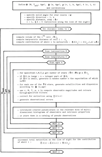
The general diagram of the new model’s mevol(code model name) constitution can be found in Fig. 2.7. Before explaining in detail its ingredients, let us shortly discuss the scheme of the star production history.

The BGM presented here is based on the new approach to the star production philosophy. As explained in the section 2.1, our starting point was a model which is based on fixed Hess diagrams for each population (Robin et al. (2003)). Its internal loop is the summation on the Hess diagram. Our main goal was getting rid of those fixed Hess diagrams and turning the IMF, SFR and evolutionary tracks into the free user-specified parameters. That meant constructing a model which takes the scenario of star creation process throughout the age of the Galactic disc, the IMF, SFR and age-metallicity relation, and using some particular sets of evolutionary tracks, extract from them the necessary information during the run time and create stars, reject the dead ones and save those which can be observed at present. In practice, to build a Galaxy from the fundamental building-blocks, we had to reconstruct the previous model and apply important changes in the code arrangement. That required to understand well the underlying relations between all mentioned components.

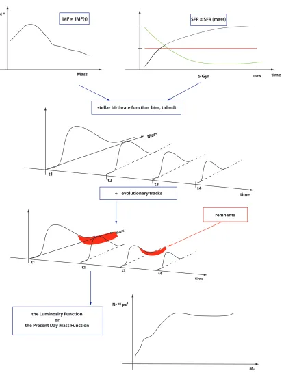
Consider Fig. 2.8. This is the graphical representation of the relationships between the theoretical IMF, SFR, evolutionary tracks and the observed LF (luminosity function) and the PDMF (present-day mass function).

The stellar birthrate function b(m, t)dmdt (see Tinsley (1976)) gives the mathematical de-scription of the star production process. It defines the number of disc stars born in the mass interval (m,m+dm) in the interval of time (t,t+dt). Knowing it precisely we could tell much about the evolution of the Milky Way. However, the nature of that function is unknown and due to the dependency on both variables, the time and the mass, the stellar birthrate function is not very convenient to work with. For that it is customary to replace it with the product of two independent functions, time and mass. This separation is only valid when one assumes that the ratio of stars being born in a given mass interval to those born at other mass value, is fixed in time.

mevol

COORDINATES LOOP DISTANACE LOOP

THIN DISC TREATMENT

AGE LOOP, seven subcomponents calculate reservmass calculate reservmassbin

MASS REGION LOOP, imass=1,2,3 create a star

draw mass, metallicity and age interpolate evolutionary tracks calculate star’s intrinsic parameters

or create a remnant END OF MASS REGION LOOP

END OF AGE LOOP

THICK DISC, HALO AND BULGE

POPULATION LOOP

LOOP THROUGH THE HESS DIAGRAM POINTS read the intrinsic parameters of each point

AGE LOOP

calculate the number of stars

STAR BY STAR LOOP calculate metallicity

END OF STAR LOOP

END OF AGE LOOP

END OF HESS DIAGRAM POINTS LOOP

END OF POPULATION LOOP

}

END OF VOLUME ELEMENT LOOP starobs.f

transform star’s intrinsic parameters into observables: add extinction and observational errors, redistribute stars, add kinematics, store in the output file

starobs.f

transform star’s intrinsic parameters into observables: add extinction and observational errors, redistribute stars, add kinematics, store in the output file

IMF ≠ IMF(t) SFR ≠ SFR (mass) N *

Mass _{5 Gyr} time

stellar birthrate function b(m, t)dmdt

+ evolutionary tracks

remnants

MV Nr */ pc3

the Luminosity Function or

the Present Day Mass Function

Mass

time t1

t2

t3

t4

Mass

time t1

t2

t3

t4

now

d2N =φ(m)Ψ(t)dmdt. (2.4)

Thus one can imagine the total number of stars ever produced in the disc as the product of the IMF and SFR continuous activity over the age of the Galactic disc (see the two dimensional graph in Fig. 2.8). During that process of creation stars evolve on their evolutionary tracks and populate the HR diagram. Their lifetimes depend on their initial masses and initial chemical compositions. Many of the stars created throughout the evolution of the Galactic disc have already died, or have moved to the later evolutionary stages. At the same time, among the alive stars we can observe many of the old objects, including some as old as the Galactic disc itself. This is due to the wide range of lifetimes, which the stars span. Applying the knowledge on the stellar evolution to the Eq. 2.4 one can get to know the distributions of stars, which have been already sent to the remnants pool, dead by now (objects marked in red in Fig. 2.8) and the stars expected to be still observed at present (the LF or PDMF).

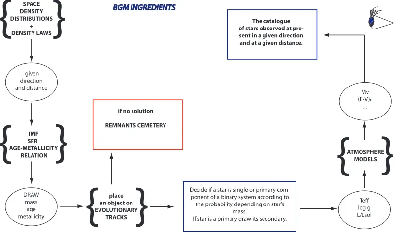
The Fig. 2.9 presents a simple scheme of the new model’s ingredients and the information they provide. The IMF, SFR, age-metallicity relation, evolutionary tracks sets, atmosphere models and space density distributions are specified previous to simulations. Firstly we draw the mass, the age and the metallicity of an object according to the chosen functions and for the obtained values we search for the solution interpolating the evolutionary tracks. If such a solution is found a star with the given L/L⊙, log g and Teff is created. Using the atmosphere models we convert its intrinsic parameters into the observed ones including the extinction effect and optionally the observational error estimations. From the a priori knowledge on the space density distributions we know how many objects are to be created at various distances within the Galactic disc. Combining all informations we get the nowadays picture of the thin disc. The stars for which the solution on the tracks was not found, meaning that the combination of their age and mass does not correspond to an alive star, have already evolved off the main sequence and giant branches and moved to the remnants cemetery. In the new BGM the remnants we consider are the white dwarfs. We neglect the density in neutron stars and stellar black holes.

That was the general scheme describing the ingredients needed to build up the evolutionary model. Now, we will explain the basic concepts of the new BGM and how we have implemented them. While in the following section 2.3, we discuss in detail the code organization.

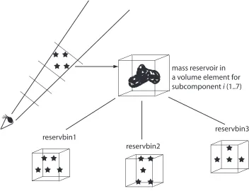
The simulations start with establishing the direction of the sky, where the star counts are going to be predicted. The most outer loops of the new code have not changed and similarly like in Robin et al. (2003) they are the coordinates and distance loops. Together they form the volume element loop. As explained in 2.1 the BGM thin disc is divided into seven age subcomponents. That division is maintained in the new model and for that the thin disc treatment is performed separately for each of these subpopulations. Once entered the age loop, the mass available to be spent on stars production in a given volume element has to be calculated. We have named this value the mass reservoir. It is an amount of mass that is expected to be found in stars at the specified position (volume element) according to the predefined evolutionary (IMF, SFR) and density (density laws) parameters. It is calculated from the formula

mass reservoir=dV ×ρ(x, y, z, i), (2.5)

Mv (B-V)o ... ATMOSPHERE MODELS

{

}

}

{

an object on EVOLUTIONARY

TRACKS

Teff log g L/Lsol

if no solution

REMNANTS CEMETERY

The catalogue of stars observed at pre-sent in a given direction and at a given distance. BGM INGREDIENTS IMF SFR AGE-METALLICITY RELATION DRAW mass age metallicity given direction and distance

}

{

{

}

DENSITY DISTRIBUTIONS

+ DENSITY LAWS

Decide if a star is single or primary com-ponent of a binary system according to the probability depending on star’s

mass.

If star is a primary draw its secondary.

Figure 2.9: The general scheme describing the ingredients needed to build the evolutionary model and the information they provide.

reasoning. Its importancy arises from the fact that it is where the star formation history, the density distributions in our Galaxy and finally the Galactic potential meet altogether. Our approach to density calculation is fully explained in the following subsection.

2.2.2 Determination of the mass model

As explained in Robin and Cr´ez´e (1986) defining the densityρ(r, l, b, i) for each age subcompo-nent irequires:

1. an estimation of the density of each component at the Sun position

2. a mathematical law capable of reproducing the trend of the density from the solar neigh-borhood to remote distances

3. evaluations of the scale heights and scale lengths of each subcomponent in order to con-strain free parameters of the mathematical expression.

The thin disc in the BGM is modelled by Einasto density laws. That mathematical model describes how the density of ellipsoidal systems changes with the distance from the Galactic center. It was chosen to represent the thin disc, because it assures the continuity and derivability in the plane. The form and associated parameters of the density laws are presented in Table 3 of Robin et al. (2003), which we discussed in section 2.1 (see Fig. 2.3).

a2=R2+z

2

ǫ2, (2.6)

where R is the galactocentric distance, z is the height above the Galactic plane, and ǫ is the axis ratio (eccentricity of the ellipsoid). It is also common to use the ellipticity parameter

e when describing the density ellipsoids. The relation between ellipticity and eccentricity of an ellipsoid is the following

ǫ=p1−e2_{. (2.7)}

In the BGM the ǫ variables for all thin disc subcomponents are obtained from dynamics considerations as it is explained later on in this section. Applying the Einasto law we calculate the relative density at the (x, y, z) position. Depending on the age subcomponent and the user’s specifications it may include the warp, flare and spiral arms influence. In order to get the absolute density one must normalize the density at the (x, y, z) position to the value at the Sun’s position.

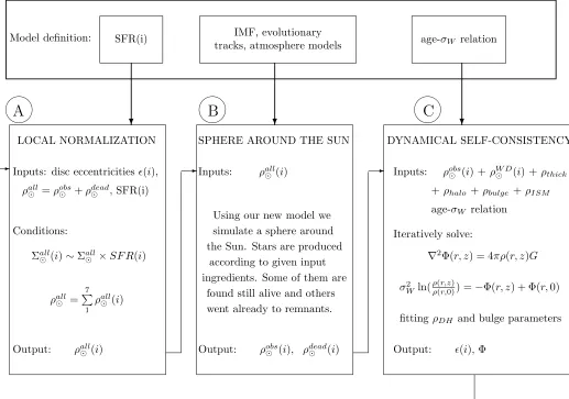
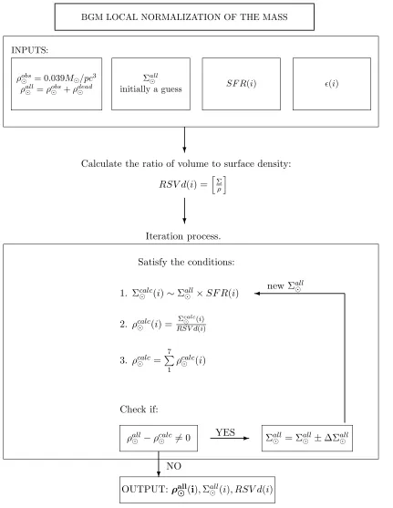
When testing new evolutionary scenarios for the Galactic thin disc the idea is to change the model’s ingredients several times. Each time we change any of the inputs we get a slightly new definition of the model leading to different results. Then, by comparing those differences we may learn what is the impact of each model’s ingredient and what are the interactions between all of them. It is important to know that each time the definition of the model changes the mass model has to be derived. Generally, the process of mass determination in our model consists of three main parts, see the scheme presented in Fig. 2.10. Block A it is a local mass normalization which provides the values of local volume density (at the Sun position) ρ⊙(i) for each age subcomponenti. Part B is where we perform the simulations of the local neighborhood and derive the percentage of alive and dead stars for each thin disc subcomponent. While in the third part C we consider the dynamics to get the parameters of the vertical density distribution. The whole procedure is a normalization iterative process, which using the observational and dynamical constraints provides the values of ρ⊙(i) and ǫ(i) and for that constructs the mass model to be applied in simulations.

As we explained at first model’s ingredients are specified. We start with the local mass normalization. A more detailed scheme for that part is presented in Fig. 2.12. The values of eccentricities ǫ(i) for each age bin i are the input for this part and they come from the potential calculations. At the beginning some guess values are assigned to them. The other inputs are the SFR, the local surface density Σall

⊙, which initially is being assigned a guess value

and local volume denisty ρall⊙, which consists of the observed volume density ρobs⊙ and a fraction

representing volume density of stars which already went to remnants. For ρobs⊙ we adopt from

observations the value of 0.039M⊙/pc3_{(white dwarfs excluded) and how we getρ}dead

⊙ we explain

in the part B. Due to the subdivision of the thin disc into seven age subcomponents the SFR is introduced to our model by the means of the intensity of star formation rate at each epoch SFR(i). Those seven dimensionless values correspond to the proportion of stars in each disc subcomponent. The way they are calculated is discussed in the section 3.2.

Model definition: SFR(i) IMF, evolutionary

tracks, atmosphere models age-σW relation

A

LOCAL NORMALIZATION

Inputs: disc eccentricitiesǫ(i),

ρall

⊙ =ρobs⊙ +ρdead⊙ , SFR(i)

Conditions:

Σall

⊙ (i)∼Σ

all

⊙ ×SF R(i)

ρall ⊙ = 7 P 1 ρall

⊙ (i)

Output: ρall

⊙ (i)

-B

SPHERE AROUND THE SUN

Inputs: ρall

⊙ (i)

Using our new model we simulate a sphere around the Sun. Stars are produced

according to given input ingredients. Some of them are

found still alive and others went already to remnants.

Output: ρobs

⊙ (i), ρdead⊙ (i)

-C

DYNAMICAL SELF-CONSISTENCY

Inputs: ρobs

⊙ (i) + ρW D⊙ (i) + ρthick +ρhalo +ρbulge +ρISM

age-σW relation

Iteratively solve:

∇2_{Φ(r, z) = 4πρ(r, z)G}

σ2 Wln(

ρ(r,z)

ρ(r,0)) =−Φ(r, z) + Φ(r,0)

fittingρDH and bulge parameters

Output: ǫ(i), Φ

-? ? ?

DETERMINATION OF A MASS MODEL IN THE NEW BGM.

x Sun

x GC

we perform the integration over the height of the cylinder

density law

kocham cie cachorrito de mi vida

Figure 2.11: In order to perform a normalization of the local volume density we consider a thin disc population enclosed withing the cylindrical volume perpendicular to the Galactic plane and with its axis passing through the Sun.

perpendicular to the Galactic plane and with its axis passing through the Sun, see Fig. 2.11. The normalization of the local density refers to the normalization of the volume and surface densities of each age subcomponent in the solar neighborhood. We know from observations the value of the local volume density in stars ρobs⊙ (at all ages), thus the procedure described

here is nothing but spliting that value into seven disc subpopulations according to the SFR and including the secular heating process, thus to get ρobs

⊙ (i). Due to the construction of our

model we need to consider a density of remnants at this point as well. From the density that is provided the model will create alive and dead stars according to the imposed evolutionary tracks and other parameters. That is why we introduce the ρall

⊙, whose value is enlarged such

that after simulations of the local neighborhood (part B), in the catalogue of thin disc alive stars we will get the value 0.039M⊙/pc3.

Assuming the ǫ(i) for each population and using the Einasto law we integrate the density

ρ(r, l, b, i) in the vertical direction and compute what we call the ratio of surface to volume density RSV d(i). The variables RSV d(i) are conceptually equal to scale heights. It would be correct to call them the scale heights only if we would use exponential laws for density. However, we chose the Einasto description in our model and instead of the scale heights its characteristic parameters are the eccentricities of the density ellipsoids.

Then an iterative process starts. We calculate the surface and volume stellar mass densities for all thin disc subcomponents, Σcalc⊙ (i) and ρcalc⊙ (i) respectively and sum them to get Σcalc⊙

and ρcalc⊙ . The condition one requires the surface density of each age subcomponent to be

proportional to the intensity of SFR in its corresponding age bin. The calculated total volume density ρcalc⊙ is compared to the imposed value ρall⊙ checking the fit to observations. If they are

different the local surface density will be modified slightly and all calculations will be repeated. When the iteration finishes we get the local volume density split into seven components ρall

Table 2.1 presents the inputs and outputs of the normalization process in question.

Density normalization

INPUTS

the total (all ages) volume mass density

ρobs

⊙ = 0.039 M⊙/pc3 observed in the SN (white dwarfs not included)

ρall⊙ =ρobs⊙ +ρdead⊙ the total volume mass density

in the SN including alive stars and remnants

the total (all ages) surface density in the SN; Σall⊙ initially a guess and then its value

is obtained through the fitting

SFR scenario 7 dimensionless factors normalized to unity, and corresponding SFR(i) vector reflecting the intensity of the SFR

acting during each age interval

ǫ(i) eccentricity of each density ellipsoid resulting from the dynamical-self consistency

calculations

OUTPUTS

ρall

⊙(i) the local volume mass density for each age bin;

the normalization factor needed to calculate themass reservoir ( see Eq. 2.5)

Table 2.1: The inputs and outputs of the density normalization process.

Once the values ofρall⊙ (i) are known the second part of the procedure takes place, see block

B in the scheme 2.10. We perform the simulations of a sphere around the Sun in order to get the values of local volume density of alive stars split into seven components ρobs⊙ (i). Our model

given some specific IMF, SFR, evolutionary tracks, age-metallicity relation, atmosphere models and other ingredients produces stars. Some of those stars are found to be still alive and they will be saved in the output catalogue. Others for whom the age and mass combination was not found on the evolutionary tracks are considered to be remnants. That is why in the local normalization part we are working with the total density valueρall

⊙, which is fitted in such a way

that in the output of a sphere simulations we want to find ρobs⊙ (i) = 0.039M⊙/pc3.

BGM LOCAL NORMALIZATION OF THE MASS

INPUTS:

ρobs

⊙ = 0.039M⊙/pc3

ρall

⊙ =ρobs⊙ +ρdead⊙

Σall

⊙

initially a guess SF R(i) ǫ(i)

?

Calculate the ratio of volume to surface density:

RSV d(i) =hΣ_ρi

?

Iteration process.

Satisfy the conditions:

1. Σcalc⊙ (i)∼Σall⊙ ×SF R(i)

2. ρcalc⊙ (i) = Σcalc

⊙ (i)

RSV d(i)

3. ρcalc

⊙ =

7

P

1 ρcalc

⊙ (i)

Check if:

ρall⊙ −ρcalc⊙ 6= 0

YES

-Σall⊙ = Σall⊙ ±∆Σall⊙ new Σ

all

⊙

?NO

OUTPUT:ρall_⊙(i),Σall⊙(i), RSV d(i)

same approach we give here a brief overview of those calculations.

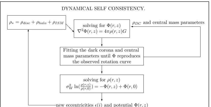
At the beginning we do not assume any a priori potential and we assign some estimated values to the eccentricities ǫ(i). The stellar content of the thin disc is simulated using the BGM (block B of Fig. 2.10) and supplemented by the thick disc, stellar halo, bulge and remaining mass components:

• interstellar matter

• dark halo

• and optionally additional local dark matter (it can be set to zero or for example it can reflect the unseen brown dwarfs).

As described in Bienayme et al. (1987) the bulge is modeled by a central point and its mass

MB is the parameter, which will be fitted. The parameters of the dark halo, which will be

adjusted are its radius rc and the central density ρc. Initially some guess values are assigned

to those dark halo and central mass parameters. All mentioned mass components enter the Poisson’s equation and impose the potential:

∇2Φ(r, z) = 4πρ(r, z)G, (2.8)

whererrefers to Galactic radius andzis the height above the Galactic plane, while Φ(r, z) is the potential andρ(r, z) is the density distribution of all included mass components. From that we get a first guess of the potential and the radial force Kr(r, z) and we move to the part where

that potential is constrained by the observed Galactic rotation curve. The circular velocity of the model is calculated from the formula:

Vcir(r) = (−Kr(r, z= 0)r)1/2. (2.9)

The central mass and corona parameters are adjusted until the potential reproduces the observed rotation curve. That results in the new potential, which satisfies the first dynamical constraint. Subsequently, it is inserted into the first order moment of the Boltzmann collisionless equation for an isothermal and relaxed stellar population (Mihalas and Routly (1968)):

σ_W2 ln(ρ(r, z)

ρ(r,0)) =−Φ(r, z) + Φ(r,0), (2.10)

whereρ(r, z) is the mass density of that population andσW its mean W velocity dispersion.

The approximation of isothermality and relaxation is fullfilled within each sub-component of the disc of age larger than 0.15 Gyr. The values of theσW velocity dispersion for each subcomponent

iare adopted from observations and are the inputs of our model , see section 3.7.

DYNAMICAL SELF CONSISTENCY.

solving for Φ(r, z) ∇2_{Φ(r, z) = 4πρ(r, z)G}

?

Fitting the dark corona and central mass parameters until Φ reproduces

the observed rotation curve

ρDC and central mass parameters

? solving forρ(r, z)

σ2 Wln(

ρ(r,z)

ρ(r,0)) =−Φ(r, z) + Φ(r,0)

?

new eccentricitiesǫ(i) and potential Φ(r, z)

ρ∗=ρdisc+ρhalo+ρISM

6 @@R

Figure 2.13: Dynamical considerations in the BGM.

2.3

The code and its implementation

2.3.1 The thin disc treatment

The BGM gives the star counts predictions towards the indicated direction in the sky. Either a line of sight or a zone can be chosen. The most outer loop is the volume element loop, thus stars are produced with distance steps while moving from the Sun till the chosen limiting value. At each volume element the objects belonging to the four basic Galactic components are generated subsequently. As explained in previous sections, we have rebuilt the thin disc treatment and here we present and discuss its new structure. We start with the general outline of the new model’s thin disc treatment, which is sketched in the Fig. 2.14.

The most outer loop of the thin disc treatment is the age loop. Each disc’s subcomponent, that is from the first to the seventh age bin is simulated separately. At small distances from the Sun the volume elements we construct are small too. In those cases the mass available to spend on stars is small as well and they lead to a tendency of creating more abundantly less massive objects than the more massive ones. Whenever the mass was not sufficient to produce a more massive star too many low mass ones were drawn and in turn it would bias the shape of the IMF. We have investigated that the bias introduced this way is significant and for that we developed two prevention mechanisms. The first one is a simple correction for the small volume elements. We enlarge the volume element by a given factor (estimated through fitting) and draw the masses from that enlarged pool. It assures that the mass calculated for that enlarged volume element is big enough for different masses to be drawn with no bias. However, not all drawn masses are kept as we have enlarged the volume element. For the further calculations we keep only a factor of drawn objects, which correspond to the original small volume element. This treatment protects from the underestimation of the stars from the high-mass IMF tail. As already mentioned, in the new model we introduce the idea of mass reservoir. The pool of mass available at the specified position within the Galactic disc is calculated from the formula 2.5 splitting it into seven subcomponents. As explained in the previous section ρi(x, y, z) is

obtained taking into account the density law, SFR and secular heating corresponding to a given i-th subcomponent and local mass normalizations. Then, the mass reservoir expressed in M⊙ and calculated for a given volume element and disc subcomponent is divided into three bins corresponding to three IMF ranges, see section 2.3.1. By construction our model works with three mass ranges and it permits introduction of at most three-slope IMF. In practice it means that the IMF can have one, two or three slopes and previously to simulations it will be divided into three ranges. Consider Fig. 2.15. This division is our second prevention mechanism against underestimating the high-mass stars and biasing the IMF. The drawing of the stars is done separately for each mass region starting always from the high mass area, then moving to intermediate masses and finishing at the low masses (see the mass range loop in Fig. 2.14). In order to divide the mass reservoir into three parts corresponding to three IMF regions we have derived formulas for the mass normalization factors. They are presented in 2.3.1.

THIN DISC TREATMENT

AGE LOOP (1..7)

END OF AGE LOOP

• calculating the correction for small volume element

• calculate RESERVMASS (1..7) - the mass available to spend at the given volume

element and within the given age bin

• calculate RESERVMASSBIN (1..3) - the pool of mass corresponding to a given

mass

MASS RANGE LOOP (1..3)

END OF MASS RANGE LOOP

UNTIL (RESERVMASSBIN (1..3) > 0)

CONTINUE

• draw a mass of an object from IMF

• Poisson statistics for small numbers:

if (mass) <= RESERVMASSBIN create a star

else apply Poisson statistics: A) do not create a star B) create a star

set RESERVMASSBIN = 0

IF A STAR IS CREATED

END IF

• draw age of an object inside of a given age interval (1..7)

• draw metallicity

• redistribute a star in a given volume element • interpolate the evolutionary tracks

IF A STAR IS ALIVE

END IF

• calculate star’s intrinsic parameters

• decide if star is single or a primary of a double system

• calculate star’s observables, add extinction effect and errors, save a star in the output catalog

• if a star is primary create its secondary, place it on

evolutionary tracks, calculate its intrinsic and observable parameters, write it to the catalogue of secondaries

RESERVMASSBIN = RESERVMASSBIN - star’s mass

ELSE A STAR IS A REMNANT

• RESERVMASSBIN = RESERVMASSBIN - star’s mass

• add a star to remnants

V V

V V V

mass reservoir in a volume element for subcomponent _i (1..7)

reservbin1

reservbin2

reservbin3

V V

V

V V

V

V V V

V V

V V

Figure 2.15: The mass reservoir calculated in the given volume element and for a given disc subcomponent is divided into three bins corresponding to three IMF ranges, which will be high mass area, intermediate and low masses. By construction, our model permits introduction of up to three-slope IMF.

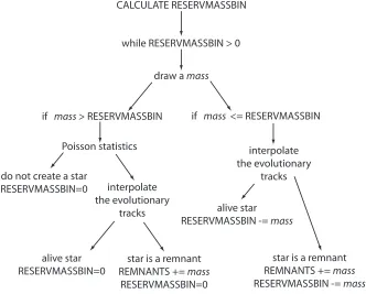
to the remaining two mass regions, but with smaller rate of occurrence. Loosing that mass would after all produce a bias in the mass distribution. To correct for that we have introduced the Poisson statistics for small numbers. Our approach consists of three possible actions. If there is enough mass in the pool for the star to be created, it will be created in an ordinary way. If the mass of drawn object exceeds the reservoir mass the Poisson statistics will be applied and as a consequence a star may be created in an extraordinary way or it might be rejected. The procedure is depicted in the tree graph in Fig. 2.16. The standard way of creating a star implies that the mass of the object will be subtracted from the total mass available to spend, while in the extraordinary case after creating the object the total mass will be set to zero. If the path of not creating a star at all is followed the mass which was left in the pool is lost and the mass reservoir is set to zero.

while RESERVMASSBIN > 0

draw a mass

if mass > RESERVMASSBIN

Poisson statistics

do not create a star

RESERVMASSBIN=0 interpolate the evolutionary

tracks

alive star RESERVMASSBIN=0

star is a remnant REMNANTS += mass

RESERVMASSBIN=0

if mass <= RESERVMASSBIN

interpolate the evolutionary

tracks

alive star RESERVMASSBIN -= mass

star is a remnant REMNANTS += mass

RESERVMASSBIN -= mass

Figure 2.16: The Poisson statistics for treating small values of mass reservoir. A star can be created in a standard way or an extraordinary way when the available resources where not enough or it can be rejected.

a primary component of a binary system. Subsequently, the observables are assigned to that object, optionally the extinction and errors are added and the star is written to the catalogue. If the produced star was flagged as a primary (see section 2.3.2) we create its secondary, place it on the evolutionary tracks, calculate its intrinsic parameters and write it to the catalogue of secondaries. The merging of binary systems is performed outside the simulations in the post processing. More details about the binarity implementation in the section 2.3.2.

We proceed producing stars subsequently from the three mass ranges as long as there is mass left in the given pool. The procedure continues for all age subcomponents and for all volume elements.

We have chosen the standard power law as the IMF representation

φ(m) =m−(1+x)_{, (2.11)}

wheremis the mass andxis the slope. It is also common to denote (1 +x) asαparameter, so then we have

φ(m) =m−α_{. (2.12)}

m1 m2 m3 m4 slope x

1

slope x 2

slope x 3

log m log z(m)

NInt1 NInt2

NInt3

Figure 2.17: Schematic representation of IMF. By construction our model works with three mass ranges and it permits introduction of at most three-slope IMF.

N Inti = mi+1

Z

mi

φ(m)dm=

mi+1

Z

mi

m−_(1+x)

dm= 1

−xi

m−xi

i+1 −m

−xi

i

. (2.13)

N Int1,N Int2 and N Int3 depicted in Fig. 2.17 are the integrals corresponding to the three

areas bounded by the IMF and their values express the number of objects in each mass range. Those values are used to draw the mass of each particular star.

IMF subroutine - draw mass of a star

Given:

• a random numbera →(0;1)

• imass range

draw a mass of a star

if (i==3) draw from [m3;m4]

elseif (i==2) draw from [m2;m3]

else (i==1) draw from [m1;m2]

Return amass

Subsequently, we show how we have derived the expression to draw the mass of an object in each mass range. Our IMF from the Eq. 2.11 is a 1-dimensional distribution function. We impose that

∞

Z

0

φ(m)dm= 1. (2.14)

Then, we define the normalized, cumulative distribution function

F(m) =

m

Z

−∞

φ(m)dm=

m

Z

−∞

m−(1+x)_{dm, (2.15)}

and after integrating we get

F(m) = m

−x

−x =

mφ(m)

−x . (2.16)

We create a random realization of a uniform probability distribution inF and we use it to draw a mass of an object

m−x

−x =

m−x

1

−x +a

m−x

2

−x −

m−x

1

−x

, (2.17)

whereais a random value from a range (0; 1i. Then, by multiplying both sides by (−x) we have

m−x_=m−_x

1 +a m

−_x

2 −m

−_x

1

so to draw the mass mwe use the expression:

m=

m−xi

i +a m

−_xi

i+1 −m

−_xi

i

−1/xi

(2.19)

for i = 1,2,3, each of the mass intervals. Using Eq. 2.13 we have

m=

m−xi

i −a xi N Inti

−1/xi

. (2.20)

On the other hand, to get the mass locked within each mass interval one must solve

Z

m φ(m)dm=

Z

m m−(1+x)_{dm (2.21)}

for all three ranges. The sum of those three numbers must be normalized to one such that

Z m4

m1

mφ(m)dm= 1 (2.22)

wherem1 andm4are the minimum and maximum masses between which the IMF is defined.

In order to fulfill the continuity condition it must occur that:

m φ(m2) =K1m

−(1+x1)

2 =K2m

−(1+x2)

2 (2.23)

and

m φ(m3) =K2m

−_(1+x2)

3 =K3m

−_(1+x3)

3 . (2.24)

K1,K2 and K3 are the continuity coefficients and they have such values that

K1

Z

m φ(m1)dm+K2

Z

m φ(m2)dm+K3

Z

m φ(m3)dm= 1. (2.25)

Thus the relative mass locked within each mass interval is computed as:

Ki

Z mi+1

mi

mφ(m)dm=M Inti. (2.26)

As explained in the previous subsection, the mass reservoir needs to be divided into three parts. This imposes a requirement that the normalization must be done on the mass and it is achieved by applying the Eq. 2.26. The sum of those values is normalized to one, so when we multiply themass reservoir (total mass in a given volume element) by each of them we distribute the available mass over three ranges in a given volume element for a given subpopulation.

2.3.2 Binarity

The new Besan¸con Galaxy Model is not any more a generator of single stars only, but it produces binary systems as well. We have implemented the binarity in the code following the scheme proposed by Arenou (2010), which is applied in the Gaia simulator. The procedure is quite straightforward, see the core of the thin disc treatment in Fig. 2.14. The age, mass and metallicity of an object are drawn and then it is placed on the evolutionary tracks. If the star is found to be alive, we calculate its intrinsic parameters and decide if it is single or a primary component of a double system. This decision is made according to the probability, which depends on the object’s mass and luminosity class, see section 3.4. At this stage a star is marked by a flag if it is single or a primary component of a double system. If the star, which has just been created was a primary, we subsequently create its secondary and this is achieved in few steps. First, the separation of the system is estimated. Next using a first guess secondary mass and system’s separation the period is calculated from the Kepler’s third law. Then, knowing the period and the M1 mass of the primary we derive theM2 mass of the secondary. We perform a

check if there is enough mass in the corresponding mass reservoir to create the secondary star. If the mass left in pool is not sufficient to create a secondary object, the primary is converted into single star and if the secondary is created successfully we assign it the same age and the same metallicity as of primary object. Then the observables of the primary are calculated and it is written to the catalogue. Similarly like for the primary component, the secondary is placed on the evolutionary tracks and its intrinsic parameters are determined. We are not considering interactive binaries which have perturbations on their evolutionary tracks due to the presence of the primary. In our algorithm the secondary star will always be found alive since at that point it was already checked that its primary which is more massive is alive. Then we derive the observables of the secondary star and save it in a separate catalogue. In our scheme merging of systems is done outside the model in the post processing. That is why if the binarity option is switched on by the user two catalogues will be created, one with single and primary stars and other with secondary components. As well the extinction effect and photometric errors will not be added directly in the simulations but saved in the catalogues. They will be applied in an independent merging code. As explained above during simulations each binary system is assigned a separation. In order to decide whether it will be resolved or not, we first randomly incline it with respect to the line of sight and then project the system on the sky. Subsequently the angular separation is computed and the decision if the system is going to be merged or separated depends on the imposed resolution of the catalogue.

In the future the merging part can be incorporated into the model, however at the moment such an arrangement has a quite convenient advantage, namely it allows us to apply several catalogue spatial resolutions to one simulated sample.

a) A sphere of 100 pc radius around the Sun.

b) The age distribution of a 100 pc radius sphere.

Figure 2.18: Simulations with a sphere mode. Option added to the model for fitting the simu-lations to the local luminosity function.

2.4

New processing modes

The BGM has several different modes in which simulations can be performed and stars created. One can choose between histograms of star counts, stars along a line of sight or in the zone of the sky, integrated light or densities on the line of sight. Since in our project we are work-ing with stars production concepts we have encountered a strong need of performwork-ing a volume limited simulations in the SN. Especially there are two cases when we were interested in lim-iting our samples by its volume, when reproducing the local observed luminosity function and reconstructing the imposed SFR.

In the task of fitting the local luminosity function one usually considers a sphere at the Sun, while for studying the SFR a cylindrical volume centered at Sun is the best. Inspired by that we have incorporated two new processing modes inside the model, such that we can simulate a sphere or a cylinder centered at the Sun position.

THE SECULAR HEATING t GC (1) (2) SFR tests

rho = 0.039 Msol/pc3

CYLINDER

ALIVE % DEAD %

SPHERE

ALIVE % DEAD %

≠

Figure 2.19: A concept of two new processing modes for stars production. A sphere is used to reproduce the local volume density and to test the LF, while a cylinder is used to test if a model is able to reproduce an imposed SFR.

an example of sphere of a radius 100 pc simulated around the Sun and in Fig. 2.18 b the age distribution of this sample.

As the sphere mode is a perfect tool for the task of luminosity function reproduction, it is a completely wrong approach when testing the SFR. Even if one would consider all stars ever born within a sphere around the Sun, one would not reproduce the original SFR when looking at their age distribution, because of the disc heating process and its dependence on scale heights. Stars are born within the plane where the gas is and then throughout their life, with each revolution around the Galaxy center their orbits get more elliptical and the corresponding velocity dispersion increases as well as the scale height. This is why the higher from the plane we move the older stars we find or in other words the old stars are supposed to be spread vertically more than the young stars. More massive stars live shorter than low mass objects thus we observe the high-mass stars strongly concentrated towards the Galactic plane, while low-mass stars are found within the plane and several parsecs outside the disc. In order to recover the SFR (which represent the value at birth) we need to deduce the distribution of stars in age after the secular heating has taken place, and at different height from the plane. This is done by correcting the number of stars of each age in the Galactic plane from the SFR, which gives the values as integrated in the solar cylinder (perpendicular to the Galactic plane and with its axis passing through the Sun). Then the number of stars of a given age at different heights will be computed from the new distribution in age at z=0 multiplied by the density law (which depends on the age).

test if a model is able to reproduce an imposed SFR.

When simulating a cylindrical volume we need to go high enough to cover all seven disc subcomponents. As they differ in ages, the oldest will be found furthest from the plane. In Fig. 2.20 a you can see an example of a simulated cylinder.

Although in simulations we have set the maximum height of a cylinder to 5 kpc, we see a strong drop in density of stars already at 2 kpc. It will depend on the scale heights or eccentricities imposed in the model, but 3 kpc seems to be fair enough for the values of scale heights we have tested in our model.

a) cylinder [-5 kpc, 5 kpc]

b) the age distribution of cylindrical volume

c) age distribution: remnants (blue) and alive stars (green)

The update of model’s inputs

We remind that our work was dedicated to the thin disc, thus all presented considerations refer to that population only.

3.1

The Initial Mass Function

We have tested several scenarios of the IMF in our simulations. Below we give a list of the ten most interesting IMF that have been applied, five are from the literature and the other five are our propositions. All the considered IMFs have a power-law form presented in the Eq. 2.12 and they differ only in the number and values of slopes and corresponding mass ranges.

1. Haywood et al. (1997a)

α=

 



1.7 0.09≦M/M⊙ <1.0 2.5 1.0≦M/M⊙<3.0 3.0 3.0≦M/M⊙<120

2. Haywood et al. (1997b) + correction of one slope in Robin et al. (2003), hereafter called Haywood-Robin

α=

1.6 0.09≦M/M⊙ <1 3.0 1≦M/M⊙≦120

3. Vallenari et al. (2006) + our extension of mass range their original function:

α=

1.1 0.2≦M/M⊙<0.8 2.3 0.8≦M/M⊙≦120

and because they do not specify the slope for masses below 0.2 M⊙, we simply extended the mass range to 0.09 M⊙:

α=

1.1 0.09≦M/M⊙<0.8 2.3 0.8≦M/M⊙≦120

4. Kroupa (2008)

α=

1.3±0.3 0.09≦M/M⊙<0.5 2.3±0.5 0.5≦M/M⊙≦150

5. Just and Jahreiß (2010)

α=

 



1.25 0.09≦M/M⊙<1 2.35 1≦M/M⊙<2 3.0 2≦M/M⊙≦100

6. Kroupa-Haywood v1

α=

 



1.3 0.09≦M/M⊙ <0.5 2.3 0.5≦M/M⊙<1.53 3.0 1.53≦M/M⊙ ≦120

7. Kroupa-Haywood v4

α=

 



1.3 0.09≦M/M⊙<0.5 2.3 0.5≦M/M⊙<1.53

3.5 1.53≦M/M⊙≦120

8. Kroupa-Haywood v6

α=

 



1.3 0.09≦M/M⊙<0.5

1.8 0.5≦M/M⊙<1.53

3.2 1.53≦M/M⊙≦120

9. Kroupa-Haywood v7

α=

 



1.3 0.09≦M/M⊙ <0.8

2.3 0.8≦M/M⊙ <1.53 3.0 1.53≦M/M⊙ ≦120

10. Kroupa-Haywood v8

α=

 



1.1 0.09≦M/M⊙<0.5

2.1 0.8≦M/M⊙<1.53 3.0 1.53≦M/M⊙≦120