C
C
|
E
E
|
D
D
|
L
L
|
A
A
|
S
S
Centro de Estudios
Distributivos, Laborales y Sociales
Maestría en Economía
Universidad Nacional de La Plata
Inequality in Health Coverage, Empirical Analysis
with Microdata for Argentina 2006
Francisco Franchetti y Diego Battistón
I
NEQUALITY IN HEALTH COVERAGE
,
EMPIRICAL ANALYSIS WITH
MICRODATA FOR ARGENTINA
2006
Francisco Franchetti (CEDLAS/UNLP) Diego Battistón (CEDLAS/UNLP)
[email protected] [email protected]
Introduction
The literature on Health Economics does not usually study health coverage1 in itself but only in an indirect
way. Specifically, the approach is often focused in health coverage as an explanatory variable of other variables which are related to the current stock of health. The intertemporal influence of health coverage over the past and future health stock is clear and evidently important beyond its influence over the present health status and its effects over the probability of sickness and recovery. Therefore, it should be clear that the interest of economic agents is to optimally preserve their health status and improve it throughout their entire life. This is an important microeconomic foundation that sustains the interest to study the health coverage as one of the important explanatory factors of the health stock. This work intends to perform a descriptive study on health coverage and explore its relationship with other variables that condition and modify the probability that economic agents receive coverage.
Given the dichotomic nature of health coverage, the realization of a descriptive and conditional analysis presents a slightly different agenda than the usual one. This work is organized in the following way: Section I, utilizing microdata from the encuesta permanente de hogares (EPH) for the first semester of 2006 in
Argentina, summary statistics are presented and a general description of the health coverage in Argentina for the people who belong to families without salary workers in it. In section II a binary regression model is estimated, and the probability of having coverage is studied. Subsequently, a Concentration Index is calculated on an individual basis. Next, following an adapted methodology than Wagstaff-Doorslaer-Watanabe (2002), a decomposition of the explained part of index which generates the probability of coverage is performed. In Section III, a decomposition of the change in the Concentration Indexes between years 2004 and 2006 takes place, utilizing microdata from the EPH corresponding to the first semester of 2004.
Intrinsic Importance of Health Coverage
Theoretical foundation
The generation of a complete theoretical model establishing a formal relationship between health coverage and the intertemporal stock of health is beyond the scope of this work. However, it is important to insure a clear understanding from the reader of why it is conceptually important to study health coverage. If we understand health as one of the ultimate goals of wellbeing for human beings, the intuitions that make the variable of coverage become clearer. Although the health status depends strongly on the behavior of individuals, it is undoubtedly true that such behavior also presents an intrinsic random component. Health coverage therefore implies an improvement over the intertemporal stock of health. More clearly, if it is accepted as it is usual in part of the literature, that health is a continuum related to life quality (health as a continuously measurable good that produces utility directly), then health coverage allows maintaining such a stock elevated because it ensures a faster recovery during and after diseases and ultimately improving life quality.
It is also usual to study health coverage as a determinant of the probability of disease in contexts of asymmetric information. Econometrically, the variable is used to estimate models of censored data. Besides this informational effect, the stock of health that it is maintained in a determined moment of time also influences the probability of disease. If health coverage has an impact over such a stock as it was established before, then it also impacts indirectly on the probability of disease independently from the moral hazard problem that it generates. Notice that the interest in this work does not lie in the development of a model that explains the probability of disease as it is usual. Even if health coverage acts against the health stock through
the negligence that moral hazard brings, in overall the economic agent who is entitled to the use of the insurance improves his well being compared to someone who does not have it. The fact that the agent might substitute some health (by raising the probability of disease through careless behavior) over other goods such as riskier recreation is irrelevant. Health coverage is valuable for economic agents and its study as an outcome variable is as valuable as the study of income or any other of the components of the multidimensional concept of welfare.
Leaving aside the moral hazard effect previously mentioned, the intrinsically random component of disease ensures a positive effect of health coverage over the stock of health over time. Given that the concept of health is also multidimensional, the health stock has an impact on at least two distinct dimensions of health. The first dimension is that the stock of health is one of the dimensions in which health is measured by itself. The second dimension of health influenced by the stock is related to the change in the probability of disease, understanding disease as a temporary but strong absence of health. Notice how health is defined as an abstract concept which is multidimensional and basically composed of the probability of disease and the stock of health. We imply that a person is healthier both when it has a larger stock of health (which could be reflected in the vitality and resistance of a person) and also when she is not sick. These two concepts are two separate dimensions of the abstract concept of health. Summarizing, it is important to realize how a larger stock of health modifies the probability of contracting a disease and how it has a direct and indirect effect over health as a source of well being.
Endogenicity of health coverage
In spite of the fact that the decision to have health insurance is strongly endogenous, studying it under a distributive perspective is never the less important. Income is also an endogenous variable in many senses. However, both for coverage and income, the continuous study of its distribution and determinants allows the isolation of those inequalities that are considered to be discriminatory or unacceptable for a determined society. The ultimate policy goal underlying this line of analysis is to provide information to allow the modification of the portion of inequality that is considered uneven and unjust for a society.
Population of Study
Considering the particular structure of health coverage in Argentina, the decision was made to exclude laborers (salary workers) and their families from the analysis. The reason is that laborers in Argentina receive mandatory coverage by law. It is also usual that the coverage to be extended for the family group. Laborers usually receive plans in which an extension to the family nucleus is provided for very low cost and in many cases this extension is possible without the requirement of being a blood relative to the laborer. By restricting the universe of study, we can isolate the relationship between coverage and other variables when these variables play a true role in the decision of being covered. The analysis of whether a Mandatory Social Security service for laborers is efficient or convenient is beyond the scope of this work.
Similarly to the mandatory provision of coverage for laborers, the elderly also have access to health coverage in Argentina when they are retired, although the provision of this coverage is not automatic or mandatory as it is for laborers. It would be natural to restrict the population of analysis to be for people who are not retired. However, some of these people do not exercise their right to be covered so that it is not always true that people who present incomes proceeding from retirement have health coverage. For these reasons, a control variable is used in the econometric models when required to capture differential effects but the population of interest is not altered.
Section I. Descriptive Analysis
In this section we perform a short characterization of the population of study utilizing traditional tools from economics of distribution.
Income and Coverage
Table I.1
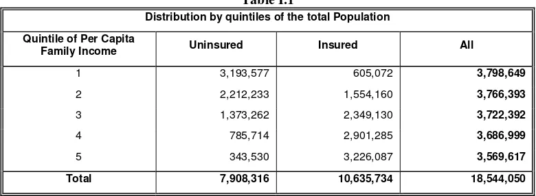
Distribution by quintiles of the total Population Quintile of Per Capita
Family Income Uninsured Insured All
1 3,193,577 605,072 3,798,649
2 2,212,233 1,554,160 3,766,393 3 1,373,262 2,349,130 3,722,392
4 785,714 2,901,285 3,686,999
5 343,530 3,226,087 3,569,617
Total 7,908,316 10,635,734 18,544,050
Source: Own elaboration based on Household Survey Data.
A marked tendency to concentrate uncovered population relative to the covered population in the first quintiles generates initial intuitions about the way in which income is related with coverage. This structure is not unusual in similar studies. From table I.1 it can be seen that between 55 to 60 percent of population. As it is seen in table I.2, the basic structure of table I.1 is preserve for the restricted population of interest although the representativity is greatly reduced to 4 millions of individuals. A great proportion of the population is excluded when the relevant restrictions are imposed. However, the pattern that emerged for the total population is preserved for the restricted sample. There is a great degree of concentration of people in the lower quintiles who do not have coverage, compared to the covered ones. This situation is reverted for the third quintile and this reversion is intensified in the upper two quintiles. The total coverage rate for the restricted sample is smaller than for the whole population as expected, representing around 52.4% of it.
Table I.2
Distribution by quintiles of Non Laborers Families Quintile of Per Capita
Family Income Uninsured Insured All
1 970,237 181,445 1,151,682
2 515,914 315,706 831,620
3 291,089 507,351 798,440
4 177,975 646,644 824,619
5 95,195 606,431 701,626
Total 2,050,410 2,257,577 4,307,987
Source: Own elaboration based on Household Survey Data.
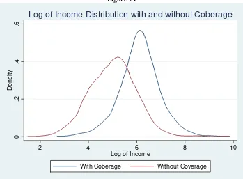
The importance of the income variable for this work is superlative. First, it is the welfare variable used to order individuals in the construction of concentration curves, it is the best available measure of welfare reported in household surveys, and it is the most important variable to be analyzed in any distributive study. The Per Capita Family Income (PCFI) was selected mainly because of its simplicity and its proved acceptance in the literature. In figure I.1 two density distributions of the PCFI are presented for the groups of covered and uncovered individuals within the relevant population of study. The distributions were estimated with the kernels method with a band2 of 0.4.
[image:4.595.106.500.376.522.2]
Figure I.1
0
.2
.4
.6
Density
2 4 6 8 10
Log of Income
With Coberage Without Coverage
Log of Income Distribution with and without Coberage
Source: Own elaboration based on Household Survey Data.
Coverage and Demographic Characteristics
[image:5.595.135.477.431.515.2]Table I.3 presents information with the means of the three socio-economic variables which are mostly examined and which are conceptually linked with the probability of being insured. All the tables in this subsection are restricted to the population of interest.
Table I.3
Demographic Characteristics of Covered and Uncovered Individuals Average Per Capita
Family Income Average Age
Average Years of Education
Insured 507.5 52.5 9.1
Uninsured 214.6 28.4 6.8
Source: Own elaboration based on Household Survey Data.
The difference between the two groups is very important for the variables selected. First, the people with higher incomes, usually of an older age, tend to have higher levels of coverage than the poorer and younger ones. Additionally, people with higher levels of education tend to present higher levels of coverage. It might appear at first sight that the average years of education for non covered individuals are high, but for a country with elevated rates of literacy like Argentina, 6.8 years is a relatively small number. However, when the calculation is restricted for the population over 18 years of age, the difference is greatly reduced to 9.92 and 9.07 years, implying that the relative proportion of children in the non-covered subgroup is higher than in the other. Also of interest, the average age of the subgroups is closer when retired people receiving a pension are excluded from the sample, and the average ages become 37.29 and 27.76 respectively.
Concentration Curves
similar procedure is performed by creating regional groups. For each province in Argentina, the average coverage rate is calculated. Next, the provinces are ordered according to their average PCFI and the values are used to construct a third concentration curve.
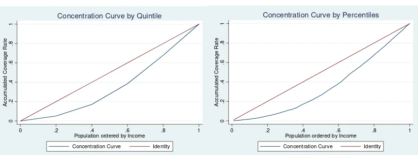
[image:6.595.91.522.191.351.2]Concentration Curves of the coverage rate by quintiles and percentiles of average PCFI. Figure I.2 presents the concentration curves by quintiles and percentiles. Although the second curve presents a softer form because of the increased number of observations, the general information provided by both of them is similar. There is evidence that the most important departure from the 45º line is produced in the first 2 quintiles of the curve.
Figure I.2
0
.2
.4
.6
.8
1
Accumulat
ed Cover
age Rat
e
0 .2 .4 .6 .8 1
Population ordered by Income Concentration Curve Identity
Concentration Curve by Quintile
0
.2
.4
.6
.8
1
Accum
u
la
ted C
o
ver
age R
a
te
0 .2 .4 .6 .8 1
Population ordered by Income Concentration Curve Identity
Concentration Curve by Percentiles
Source: Own elaboration based on Household Survey Data.
The most important comment to make about figure I.2 is that an important part of the inequality contained in health coverage is not captured when the procedure followed to produce the concentration curves is used. The variation within quantiles is lost and naturally the results change with the election of the numbers of quantiles to be calculated. This choice is not only arbitrary but also restricted by the amount of observations available. However, complemented with the rest of the figures and measures presented in this work, the grouping by quantiles provides relevant information on the distribution of health coverage.
Concentration Curve of the coverage rate by average PCFI of the provinces
[image:6.595.173.439.536.724.2]Before the analysis of figure I.3, it is important to clarify the true informative potential of the figure. Note that the utilization of income and the average coverage rate for each region tends to distort the measures of inequality because the variation within groups is lost under this procedure. For further details on the interpretation of this figures see Sala-i-Martin (2006).
Figure I.3
0
.2
.4
.6
.8
1
Accum
u
lated Coverage Rate
0 .2 .4 .6 .8 1
Provinces ordered by Average Income
Concentration Curve Identity
Concentration Curve by Provinces-Conglomaerates
As it is evident, inequality in the levels of health coverage is strongly reduced when regional units are used as observations implying that there is great heterogeneity within the regions which was captured by the quantiles grouping and eliminated by the regional grouping. Methodologically, this result suggests a warning over studies which calculate only indicators based on regional grouping. It also reinforces the always present principle that values and figures in distributive analysis are more valuable when analyzed in the appropriate context comparing them with other measures and indicators. In line with this methodological approach, later in this work an intertemporal analysis of some of the measures and figures is performed.
The study of the regional distribution of coverage and the identification of the conglomerates and provinces with lower distributive performance in health coverage are not part of the scope of this work. The presentation of the concentration curve at a regional level represents only part of the multiple approaches to study the distribution of health coverage in Argentina as a whole.
The calculation of the regional curve is based in micro data from 23 conglomerates. The criterion followed was to take the most important conglomerate in each province although this was not possible in the case of Neuquén and Rio Negro, provinces for which a common conglomerate is used in the survey.
Section II. Derivation and Decomposition of the Coverage Index of
Inequality (CII)
This section has two clearly defined objectives. First, we obtain an indicator that measures inequality in health coverage at an individual level. Second, we decompose such an indicator in parts that reflect the individual conditional impact of a group of explanatory variables on the index. In this way, partial magnitudes for the index can be attributed to specific variables, conditional on the rest of the controls in the model. This procedure is an adaptation for binary models of a previously existing linear method presented in Wagstaff-Doorslaer-Watanabe (2002).
It is necessary to stress a few points that must be considered before proceeding with the empirical analysis regarding any estimation strategy and interpreting the results. First, the health variables have a major unobservable component which depends on biological and intrinsically random circumstances and are independent of any socio demographic variable such as income or the education level. Second, there is no consensus among the different authors in the literature on a theoretical model that would satisfactorily and completely explain the behavior of health variables. Finally, the empirical literature is not homogeneous in the variables used, the explanatory capacity of the models is usually low (especially when it is based in survey data regressions) and to obtain the most accurate results in terms of methodology, panel data are required, which are unavailable in most Latin American countries, Argentina included. Considering all these elements, we find it convenient to perform the analysis without resorting to any causality hypothesis between the studied variables.
Regression Analysis
In the Economics of Health literature, it is common to utilize categorical or binary variables to measure the state of health or some other variable like health coverage. For a revision of the econometric tools which are normally used, we refer the reader to Jones (1998). Here, we follow the procedure of obtaining a continuous coverage index estimating a probit model over the health coverage variable. The election of the complete set
of variables in the estimation was performed on the basis of their previous interest in the literature (see Gerdtham, U-G. Johannesson, M. (1997)). Additionally, we include some demographic variables such as the size of the home of the individual, the number of children in the house and the marital status (married or not married). To contrast the hypothesis that regional inequalities exist between provinces and to capture a portion of the inequality detected visually in figure I.3, we include dummy variables for each region in the country3. In Table II.1 a succinct description of the utilized variables is presented.
3 To test the heterogeneity of the groups of individuals covered and not covered in related to the group of variables
Table II.1
Variable Description lipcf Logarithm of the PCFI
aedu Years of Education edad Years of Age edadsq Squared Years of Age
hombre Dummy variable with value one for men.
casado Dummy variable with value one if the person is married miembros Number of members in the Household of the individual miembrossq Squared number of members
nro_hijos Number of children present in the household of the individual nro_hijossq Squared Number of children
jubilado Dummy variable with value one if the person is retired and receiving a pension ocupado Dummy variable with value one if the person is employed
nea Regional Variable for Region Noreste noa Regional Variable for Region Noroeste pampa Regional Variable for Region Pampeana cuyo Regional Variable for Region Cuyo pata Regional Variable for Region. Patagonia
Source: Own elaboration.
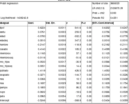
In Table II.2 the estimation results of the binary model are presented, were the preceding variables act as regressors
Table II.2
Probit regression Number of obs 3666020
LR chi2(13) 2126870.39
Prob > chi2 0.000 Log likelihood -1438242.8 Pseudo R2 0.4251
dsegsal Coef. Std. Err. z P>z [95% Conf.Interval]
lipcf 0.6224 0.0011 541.6 0.00 0.6202 0.6247
aedu 0.0761 0.0003 293.0 0.00 0.0756 0.0766
edad -0.0783 0.0003 -302.2 0.00 -0.0788 -0.0778 edadsq 0.0010 0.0000 347.2 0.00 0.0010 0.0010 hombre -0.2147 0.0018 -118.8 0.00 -0.2182 -0.2111 casado 0.4143 0.0022 185.2 0.00 0.4099 0.4186 miembros 0.1165 0.0020 57.1 0.00 0.1125 0.1205 miembrossq -0.0116 0.0002 -51.6 0.00 -0.0121 -0.0112 nro_hijos -0.0533 0.0017 -30.9 0.00 -0.0566 -0.0499 nro_hijossq 0.0051 0.0004 14.4 0.00 0.0044 0.0058 jubilado 1.4118 0.0033 426.5 0.00 1.4053 1.4183 ocupado -0.3271 0.0023 -144.7 0.00 -0.3315 -0.3226
nea 0.0366 0.0036 10.1 0.00 0.0295 0.0438
noa 0.1697 0.0029 58.0 0.00 0.1639 0.1754
pampa 0.1800 0.0021 86.2 0.00 0.1759 0.1841
cuyo -0.0602 0.0032 -18.6 0.00 -0.0666 -0.0539
pata 0.0965 0.0054 17.8 0.00 0.0859 0.1071
intercept -3.5246 0.0096 -368.8 0.00 -3.5434 -3.5059
[image:8.595.93.521.397.742.2]The general fit of the model is satisfactory in the overall. Extraordinarily, all the variables are significant at 99 percent of confidence. For a binary model based in microdata, the adjustment is surprisingly important. Although the measures of goodness of fit present issues in binary models, the pseudo R2 of 0.42 should be
considered as relatively satisfactory for a probit model. Notice how the squares of the variables for members, children and age capture the tradition nonlinear relationship between these variables and the probability of coverage.
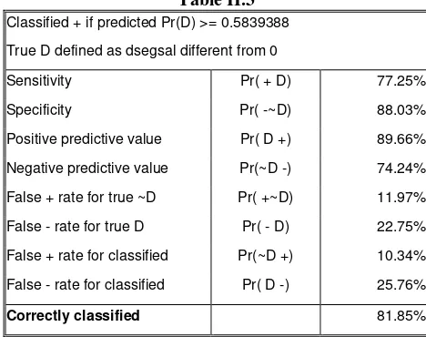
[image:9.595.186.420.204.389.2]Complementary to the estimation results, in table II.3 we present resumed information regarding the predicted power of the model which is a second way to assess the goodness of fit of the model. The cut point for correct or incorrect prediction is chosen as the proportion of individuals with coverage and not in 0.5. The value is calculated for all the population of interest without dropping the missing values from the regressors. ,
Table II.3
Classified + if predicted Pr(D) >= 0.5839388 True D defined as dsegsal different from 0
Sensitivity Pr( + D) 77.25% Specificity Pr( -~D) 88.03% Positive predictive value Pr( D +) 89.66% Negative predictive value Pr(~D -) 74.24% False + rate for true ~D Pr( +~D) 11.97% False - rate for true D Pr( - D) 22.75% False + rate for classified Pr(~D +) 10.34% False - rate for classified Pr( D -) 25.76%
Correctly classified 81.85%
Source: Own elaboration based on Household Survey Data.
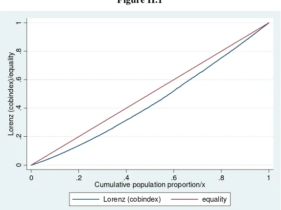
Concentration Curve
With the coefficients from the preceding model in the previous subsection, it is possible to construct an individual level variable, given by the index of the probabilistic model. Specifically, the probit model adjusts the following model for the binary variable
y
:[
|
]
Pr
(
1|
)
(
'
E y x
=
y
=
x
= Φ
X
β
)
Figure II.1
0
.2
.4
.6
.8
1
Lorenz (cobindex)/equality
0 .2 .4 .6 .8 1
Cumulative population proportion/x
Lorenz (cobindex) equality
Source: Own elaboration based on Household Survey Data.
The coverage index curve presents a smaller departure from the 45 degree line than the previously calculated curves based on quintiles. This implies that to some extent, part of the heterogeneity in health coverage is not captured by the variables in the model and remains in the residual part of the model. It is important to see that none of the procedures to calculate the concentration curves is better than the others in all the relevant aspects. Therefore, the best way to analyze the information presented is through a complementary analysis that exploits all the information presented. Also noteworthy, the tendency to concentrate the major departure from the identity line in the first 40 percent of the population (the first two quintiles) is equally present in this curve and the ones built by quantiles.
Concentration Index
Before the decomposition of the concentration index derived from figure II.1, we present the diverse concentration indexes which are derived from the curves presented earlier in sections I and II.
Table II.4
Variable Concentration Index
Probit Coverage Index (XB) 0.115 Coverage Rate by Quintiles 0.421 Coverage Rate by Percentiles 0.486 Coverage Rate by Provinces 0.347
Source: Own elaboration based on Household Survey Data.
As it was expected, due to the unexplained components in the probit model, the concentration index calculated using the continuous coverage index is remarkably lower than the one derived in any of the remaining forms. It is evident therefore, that the Coverage Index can only explain the portion of inequality
that is related to socio economic variables. This does not represent a serious problem since the indexes generated by quantiles help to understand the magnitude of the remaining unexplained inequality. Although some unobservable variables which explain a big part of coverage inequality are not available, the decomposition still allows finding interesting relationships with many relevant policy variables such as income, years of education and the rest of the variables in the model which are the most usual target of policies.
Concentration Index Decomposition
[image:10.595.160.452.473.563.2]At this point it is important to emphasize the importance of the goodness of fit in order to correctly assess the relevance of the decomposition. In a standard OLS model, the goodness of fit is relatively high and the residuals are a minor problem. In a binary model, it is possible that the explanatory power of the variables might be very small. In these circumstances the relevance of the decomposition at a policy level might turn out to be irrelevant. However, notice that most measures of concentration change only a few percentage points in a decade. Therefore, changes of one or half percentage point should be considered of importance in this context. The crucial point is that small changes in a concentration index can imply major changes in the aggregate levels of welfare in a society.
Derivation of the Decomposition
Let us suppose that a distributive variable represents the values which are accumulated in a concentration index and that
y
R
represents the rank or “standardized order” of the welfare variable (the variable that orders the observations in a concentration curve) in the calculation of the concentration index (usually income). Then, beginning with the recognized result by Kakwani (1997) we have:(
)
( )
(
)
(
)
(
2 cov ,
/
.1
2
1/ 2 /
y
y y
CI
y R
II
CI
E
y
R
II
µ
µ
µ
=
⎡
⎤
=
⎣
−
−
⎦
.2
)
)
3
In the appendix we show that (II) is equivalent to[
]
(
max min)
(
1
/
.
K
k k k y
k
CI
β µ
CI
µ
z
z
II
=
⎡
⎤
=
∑
⎣
−
⎦
where k indexes the explanatory variables of the binary model.
The result in (II.3) is interpreted as a weighted sumo f the concentration indexes of the explanatory variables (the intercept has a null index so its inclusion is trivial) in which the weights are given by the coefficients, the mean of the explanatory variables, normalized by the mean and rank of the dependent variable (this is due to the normalization performed to avoid negative values in the index.
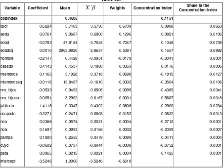
Decomposition Results
Table II.5
Variable Coefficient Mean
X
′
β
Weights Concentration Index Share in the Concentration Indexcobindex 0.4605 0.1151
lipcf 0.6224 5.7403 3.5730 0.6709 0.0988 0.0663 aedu 0.0761 9.0687 0.6900 0.1296 0.0821 0.0106 edad -0.0783 47.9184 -3.7534 -0.7047 0.1048 -0.0738 edadsq 0.0010 2863.9820 2.8657 0.5381 0.1657 0.0892 hombre -0.2147 0.4428 -0.0951 -0.0179 -0.0041 0.0001 casado 0.4143 0.4537 0.1880 0.0353 0.0176 0.0006 miembros 0.1165 3.1928 0.3718 0.0698 -0.1815 -0.0127 miembrossq -0.0116 13.8487 -0.1610 -0.0302 -0.3504 0.0106 nro_hijos -0.0533 0.9493 -0.0506 -0.0095 -0.4369 0.0041 nro_hijossq 0.0051 3.2992 0.0167 0.0031 -0.5687 -0.0018 jubilado 1.4118 0.3047 0.4302 0.0808 0.2900 0.0234 ocupado -0.3271 0.2471 -0.0808 -0.0152 0.0832 -0.0013 nea 0.0366 0.0574 0.0021 0.0004 -0.2712 -0.0001 noa 0.1697 0.0993 0.0168 0.0032 -0.2099 -0.0007 pampa 0.1800 0.2655 0.0478 0.0090 0.0411 0.0004 cuyo -0.0602 0.0737 -0.0044 -0.0008 -0.0752 0.0001 pata 0.0965 0.0215 0.0021 0.0004 0.1425 0.0001 intercept -3.5246 1.0000 -3.5246 -0.6618
Source: Own elaboration based on Household Survey Data.
From the analysis of the last column (7), it follows that income, years of education; age and retirement are the most important variables to explain the explained portion of inequality, conditional on the rest of the variables selected. Notice that the retirement variable works mainly as a control for ease of accessibility but no attempt to interpret it as capturing only social discrimination should be performed. The variable age square has the opposite sign than the linear one, indicating a neutral global effect. Something similar happens with the children variable. Summarizing, income seams like the most important variable in the decomposition.
Section III. Comparative analysis of inequality
This section attempts a comparative analysis between two moments of time for the methodology developed in section II. The data from the EPH household surveys in Argentina for years 2004 and 2006 in the first semester are used. Ideally, it would be convenient to separate the points in time several years and not only two. However, in other surveys the variable of coverage is not reported (for instance the punctual older version of EPH). Other surveys report the variable but their data is relatively old. Such is the case of the
living standards survey or Encuesta de Condiciones de Vida (ECV). Given the temporal proximity of the two
datasets analyzed, it is not expected that the changes found are big, especially considering the relative macroeconomic stability that the Argentinean economy presents in the period.
Concentration Curve
The equivalent results to the ones presented in the previous section for year 2006 are not presented here for the year 20044. The results regarding the goodness of fit and the significance of explanatory variables are
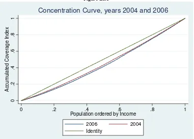
similar to those for 2006. In figure III.1 we show two concentration curves for the years 2004 and 2006 so that they can be compared.
Figure III.1
0
.2
.4
.6
.8
1
Accumulated Coverage Index
0 .2 .4 .6 .8 1
Population ordered by Income 2006 2004 Identity
Concentration Curve, years 2004 and 2006
Source: Own elaboration based on Household Survey Data.
The curves can be barely distinguished. The 2006 curve seems slightly exterior to the 2004 curve for the lower values of income, but a clear dominance can not be established for the entire curve. The methodology
used to construct the index seems to produce very similar results for the two years. This similarity can be interpreted as positive attribute since it implies a certain degree of robustness and the possibility to perform comparisons through time when enough surveys are made available.
Changes in the Concentration Index
This section represents a natural step after the uninformative power of the graphic tool presented in the previous section. Consequently, a quantification procedure is now performed to compare the concentration indexes in the two years. The calculations were performed not only for the probit coverage index but also for the other concentration indexes constructed with groups. This information is summarized in table III.1
Table III.1
Variable
Concentration Index for year 2004
Concentration Index for year 2006
Change in the Concentration Index
Probit Coverage Index Variable 0.092 0.115 0.023
Rate of Coverage by Quintiles 0.386 0.421 0.035
Rate of Coverage by Percentiles 0.452 0.486 0.033
Rate of Coverage by Provinces 0.345 0.347 0.003
Source: Own elaboration based on Household Survey Data.
[image:13.595.86.525.531.625.2]Decomposition of the Changes in the Concentration Index
In this subsection, a decomposition of the changes in the concentration index obtained in the previous subsection is performed. The decomposition is restricted to the probit coverage index obtained through the regression model.
Derivation of the change decomposition
Continuing with the notation from section II, notice first that the mean of the dependent variable is a function of the intercept and the rest of the coefficients. With this in mind, the following differences and differentials can be calculated:
[
]
2(
)
(
(
)
)
(
) (
)
max min max min 1
0 0 max min
/
1/
K y
k k k y
k
y y
d
dCI
dCI
CI
CI
z
z
z
z
III
d
d
d
z
z
.1
µ
β µ
µ
β
µ
β
=µ
⎡
⎤
=
= −
⎣
−
⎦
−
= −
−
∑
[
]
(
max min)
(
)
(
(
)
) (
)
max min max min
/
.
y k k k k
k k y
k k y k y y
d
CI
CI
CI
dCI
CI
dCI
CI
z
z
III
d
d
d
z
z
z
z
2
µ
µ
µ
µ
µ
β
β
µ
β
µ
µ
−
∂
⎡
⎤
=
+
=
⎣
−
⎦
−
=
∂
−
−
[
]
(
max min)
(
)
(
(
)
) (
)
max min max min
/
.
y k k k k
k k y
k k y k y y
d
CI
CI
CI
dCI
CI
dCI
CI
z
z
III
d
d
d
z
z
z
z
3
µ
β
µ
β
β
µ
µ
µ
µ
µ
µ
−
∂
⎡
⎤
=
+
=
⎣
−
⎦
−
=
∂
−
−
[
]
(
max min)
(
)
(
)
max min
/
k k.
k k y
k k y
dCI
CI
z
z
III
dCI
CI
z
z
4
β µ
β µ
µ
µ
∂
⎡
⎤
=
=
⎣
−
⎦
=
∂
−
Differentiating over
CI
:(
)
0 1 1 1
0
.5
K K K
k k k
k k k
k k k
dCI
dCI
dCI
dCI
dCI
d
d
d
dCI
III
d
β
β
=d
β
β
=d
µ
µ
=dCI
=
+
∑
+
∑
+
∑
Substituting (III.1) through (III.4) into (III.5):
(
)
[
]
(
)
(
)
0 1 max min.6
Kk k k k k k k k
k
y
CI d
CI
CI
d
d
dCI
dCI
III
z
z
β
µ β
β µ
β µ
µ
=⎡
⎤
−
+
⎣
−
+
+
⎦
=
−
∑
It is interesting to remark the fact that the constant term plays a role in the decomposition of the change in the indexes although it does not play a role in the absolute decomposition. An increase in the constant part of the model generates an even increase in the probit coverage index variable which affects in a larger proportion to the poorest of the individuals and generates an equalizing tendency which tends to reduce the concentration index level.
Results of the change decomposition
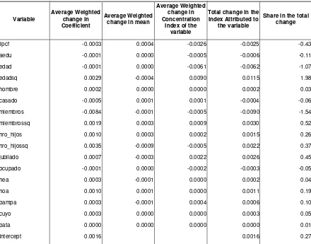
Given the inherent complexity of the calculation of the decomposition performed here, a detailed description of the steps performed would be uninformative. To summarize the composition of the change, Table III.2 presents the changes which can be attributed, according to the formula in (III.6) to changes in coefficients, changes in means and changes in the concentration index of each variable. These values are shown already weighted by the factors that influence them according to III.6. The sum of these three columns of any row represents the total impact of the variable in that row over the total change in the concentration index between 2004 and 2006.
Table III.2
Variable
Average Weighted change in Coefficient
Average Weighted change in mean
Average Weighted change in Concentration
Index of the variable
Total change in the Index Attributed to
the variable
Share in the total change
lipcf -0.0003 0.0004 -0.0026 -0.0025 -0.43
aedu -0.0001 0.0000 -0.0005 -0.0006 -0.11
edad -0.0001 0.0000 -0.0061 -0.0062 -1.07
edadsq 0.0029 -0.0004 0.0090 0.0115 1.98
hombre 0.0002 0.0000 0.0000 0.0002 0.03
casado -0.0005 0.0001 0.0001 -0.0004 -0.06 miembros -0.0084 -0.0001 -0.0005 -0.0090 -1.54 miembrossq 0.0019 0.0003 0.0009 0.0030 0.52 nro_hijos 0.0010 0.0003 0.0002 0.0015 0.26 nro_hijossq 0.0035 -0.0009 -0.0005 0.0022 0.37 jubilado 0.0007 -0.0003 0.0022 0.0026 0.45 ocupado -0.0001 0.0000 -0.0002 -0.0003 -0.05
nea 0.0003 -0.0001 0.0000 0.0002 0.04
noa 0.0010 0.0001 0.0000 0.0011 0.19
pampa 0.0003 -0.0001 0.0004 0.0006 0.10
cuyo 0.0003 0.0000 0.0000 0.0003 0.05
pata 0.0000 0.0000 0.0000 0.0000 0.01
Intercept 0.0016 0.0016 0.27
Source: Own elaboration based on Household Survey Data.
An important element to mention is that the intercept only impact through changes in the coefficient since the mean, which is always 1 and the concentration index which is always zero are not subject to variation. In general, the results indicate that the most important variables to explain the changes have been income, retirement (once again difficult to interpret) and the variables with squares. Income and the number of members (which probably decreased for demographic reasons) seem to be the two most important variables going in the opposite direction to the global change. The two most relevant variables that contribute to the increase in the concentration index are age (mainly due to a bigger concentration index for this variable) and the number of children (which probably increased due to the macroeconomic normalization)5. The rest of the
variables seem to play a relatively smaller role in explaining the changes in the index, although it is important to understand that this decomposition is conditional on every one of the variables present and the inclusion or exclusion of some of the variables could change the magnitude of the different components.
Conclusions
Methodologically, in this work we find that the methodology of constructing continuous indexes for dichotomic variables using binary models of regression captures only a fraction of the inequalities in the outcome variable. However, the analytical possibility to perform decompositions over such indexes and the availability of other complementary measures of inequality conform a set of tools that allow generating valuable information regarding the distributive nature of the variable studied.
5 The sum of the changes is not the same than the global change in the index for approximation problems and a change in
the range of values in the different surveys
(
zmax−zmin)
. Here, the emphasis of the analysis is especially linked to theFor the population and surveys studied in this work, we find that for Argentinean EPH survey, our model captures a significant although minor part of the overall level of inequality in health coverage. We find important differences between the groups of covered and not covered individuals. We also find that income is a strong cause of inequality in health coverage, once its effects are controlled by a rich number of variables. As mentioned in the beginning of this work, this result does not establish a causal relationship between the two variables, it simple evidences how strongly linked they are. The knowledge of this link is crucial in the generation of policies focused in reducing inequality in health coverage.
Finally, in an intertemporal perspective, we find that between the years 2004 and 2006 health coverage inequality was augmented as measured by all the concentration indexes. The income recovery after the macroeconomic crisis of 2001 plays a role in reducing the increase in inequality, but a number of demographic factors present nullify this effect.
Appendix
First, Notice that the mean of the rank is always ½ . The result in (II) can be rewritten in sample form in the following way:
(
)
(
)
(
1
2
1/ 2 /
N
i y i y
i
CI
y
µ
R
N
µ
A
=
⎡
⎤
=
∑
⎣
−
−
⎦
.1
)
.2
.3
)
It is straight forward to see that (A.I) can be rewritten as:
[
]
( )
1
2
/
1
N
i i y
i
CI
y R
µ
N
A
=
=
∑
−
For any explanatory variable in a binary model, expressions (A.1) and (A.2) can also be written in a similar way as:
k
x
[ ]
( )
1
2
/
1
N
k i i k
i
CI
x R
µ
N
A
=
=
∑
−
[ ]
(
)
(
1
1 / 2
.4
N
i i k k
i
x R
µ
N CI
A
=
=
+
∑
Let us now define
z
=
x
'
β
; then the standardized health index used to eliminate negative values would follow the formula:(
'
min) (
/
max min)
( )
y
=
x
β
−
z
z
−
z
A
.5
)
1
.6
)
7
)
8
Replacing (A.5) into (A.1) and rearranging:(
)
min(
max min)
(
1 1 1
2
K k N ki i N i/
yk i i
CI
β
x R
z
R
µ
N z
z
A
= = =
⎛
⎡
⎤
⎞
⎡
⎤
=
⎜
⎢
⎥
−
⎟
⎣
−
⎦
−
⎣
⎦
⎝
∑ ∑
∑
⎠
Substituting (A.4) in (A.6) and rearranging:
[
]
(
max min)
(
1
/
.
K
k k k y
k
CI
β µ
CI
µ
z
z
A
=
⎡
⎤
=
∑
⎣
−
⎦
noticing the traditional result from regression analysis:
(
min) (
max min)
(
1
/
.
K
k k y
k
z
z
z
A
Bibliography
Bertranou, Fabio., (1999), Moral hazard and prices in Argentina’s health markets, mimeo, Universidad Nacional de Cuyo.
Cowell, F. (1995). Measuring inequality. LSE Handbooks in Economic Series, Prentice Hall/Harvester Wheatsheaf. Everitt, B. S. y Dunn, G. (2001) “Applied multivariate data analysis”. 2ª ed. Edward Arnold, London.
Figueras S, M (2000): "Análisis Discriminante", 5campus.com, Estadística http://www.5campus.com/leccion/ discri Gerdtham, U-G. Johannesson, M. (1997) “New Estimates of The Demand for Health: Results Based on a Categorical Health Measure and Swedish Micro Data”. Working Paper Series in Economics and Finance. No. 205, 1-19
Hair, j., Anderson, r., Tatham, r. y Black, w. (1999). Análisis Multivariante. 5ª Edición. Prentice Hall.
Lambert, P. (1993). The distribution and redistribution of income. Manchester University Press
Wagstaff, A. (1993) “The demand for health: an empirical reformulation of theGrossman model”. Health Economics, II,