PPP, UIP and Fisher parity: speculation or
rational expectations?
Evidence for four Latin American countries
(Thesis Proposal)
Student: Nataly Obando Rozo
∗Advisor: Jesús Otero
September 11, 2013
Abstract
This work aims to test the equilibrium relations of two international macroe-conomics models for Colombia, Chile, Mexico and Brazil. The first model is the rational expectation hypothesis (REH) where three key relations will be tested: Purchasing Power Parity (PPP), Uncovered Interest Rate Parity (UIP) and the Fisher Parity condition. The second model follows the line of though of Imperfect Knowledge Economics (IKE) where two equilibrium relations will be tested. According to IKE, even under the assumption that agents are ra-tional, the presence of speculative behavior in financial markets helps explain the long swings often observed in the behavior of exchange rates. The results support the view that the predictions of the IKE model hold for Colombia, while those of the REH hold for both Brazil and Mexico. Mixed findings are obtained for Chile.
Keywords: Long Swings, Imperfect Knowledge, CVAR, Currency markets, Spec-ulation.
JEL Classification: E24, F31, F41.
1
Introduction
“All theory depends on assumptions which are not quite true. That is what makes it
theory. The art of successful theorizing is to make the inevitable simplifying assumptions
in such a way that the final results are not very sensitive... When the results of a theory
seem to flow specifically from a special crucial assumption, then if the assumption is
dubious. the results are suspect”
Robert Solow (1956)
“I confess that I prefer true but imperfect knowledge, even if it leaves much indetermined
and unpredictable, to a pretence of exact knowledge that is likely to be false”
Hayek. Nobel Prize lecture (1974)
The conventional approach to exchange rate dynamics assumes rational individ-uals interacting in a market where the driving forces of the system, or equilibrium relations, are led by the macroeconomic fundamentals (see Mundel, 1963., Fleming, 1962., Dornbusch, 1976a., Dornbusch, 1976b., Frenkel, 1976). However, the empiri-cal failures or puzzles of these macroeconomic models have opened the door to the notion that macroeconomic fundamentals may not play an important role in driv-ing macroeconomic outcomes, and thus ideas such as irrational behavior of market participants have begun to appear in the literature.
Expectation Hypothesis make sense?. Are macroeconomic fundamentals the driving forces of market outcomes?. Can policy makers influence the market?.
In order to answer these questions, this thesis follows a contemporary approach of economic analysis known as Imperfect Knowledge Economics (IKE), see Fryd-man and Goldberg (2007). The IKE model, in the tradition of early modern eco-nomics, links mathematically the aggregate outcomes with the behavior and fore-casting strategies of individuals. However, models based on IKE reflect modesty about how complete the representations of individual behavior can be.
The idea that exchange rate dynamics are driven by ’irrational noise’ traders who do not rely on macroeconomic fundamentals is not an assumption in IKE. On the contrary, the model assumes that market participants must cope with imperfect knowledge, which is not the same as the presumption that they are irrational. But when perfect knowledge does not exist, although macroeconomic fundamentals play an important role in the model, individuals speculate in their forecasting behavior and the hypothesis of rational expectation fails to hold. This approach differs from the speculative economic bubbles approach in the sense that in the IKE model, macroeconomic fundamentals play an important role by being the driving force of the system; as will be seen later, macroeconomic fundamentals are a reference point in forecasting strategies, and therefore policy makers do interact and influence the market.
to the existing literature which, to the best of our knowledge, generally tests each hypothesis separately.
This rest of the thesis is organized as follows. Section 2 briefly presents both the REH and IKE model. Section 3 presents a brief review of the literature of REH and IKE, including some empirical applications. Section 4 presents the econometric methodology and summarizes the cointegration relations that will be tested under REH and IKE. Lastly, section 5 concludes.
2
Rational Expectation Hypothesis vs. Imperfect
Knowledge Economics
2.1
REH framework
The ex-post return on a pure long position,rt+1,of an individual who invests abroad
can be written as:
rt+1 =st|t+1−st+ift −idt, (1)
where st|t+1−st is the expected change in nominal exchange rates, and ift and
idt are the foreign and domestic interest rates, respectively. For each unit of investment, an individual would get 1
St units at ift, that is the money they receive in foreign currency. Then, the next period the individual sells
1
St(1 +ift) at the exchange rate St+1 in order to get the earnings in the national currency. Therefore the total return of the long position would be St+1St (1 +ift)−
To model this return, economists assume that the exchange rate adjusts to equate demand and supply. Let rˆt|t+1 and upˆt|t+1 denote all market participants’ point forecast of rt+1 and of the premium that they require to hold an open position
in foreign exchange rate market, respectively. Equilibrium in the foreign exchange market under perfect capital mobility can be written as:
ˆ
rt|t+1 = ˆupt|t+1.
This equation holds whether individual preferences are represented as risk neutral or risk averse, or are based on prospect theory. However, the assumption of REH is that the conditional expectation rˆt|t+1 is equal to the conditional expectation of
rt+1. Further, if individual preferences are risk neutral, as generally assumed in the
REH models, thenupˆt|t+1 = 0. This leads to the conclusion that the ex-post return has a conditional mean of zero and is uncorrelated with the causal variables that an economist includes in his/her representation. The equilibrium of the REH is a no-arbitrage condition where individuals are indifferent to the interest rates available in the two countries.
With these assumptions, equation (2) is the well known Uncovered Interest Parity condition:
∆st+1 =idt−ift. (2) Another equilirbuim condition generally invoked by REH is Purchasing Power Parity (PPP). PPP asks how much money would be needed to purchase the same basket of goods and services in two countries. Then, if prices rise abroad, the exchange rate St adjusts in order for PPP to hold. Thus Pdt =St·Pft or St=
Pdt Pft. Where Pdt is the domestic price, Pft is the foreign price. Taking logs yields:
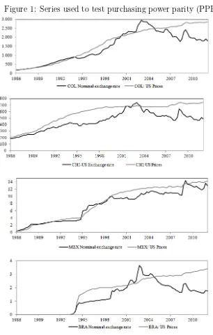
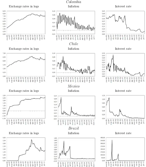
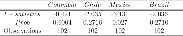
If PPP holds for Colombia, Chile, Brazil and Mexico, then one would see in Figure 1 that the black line should be equal to the gray line, or at least the difference is stationary. With the series in logs. Table 2 shows the results of applying Dickey-Fuller test to the real exchange rates of the countries under consideration. The results suggest that for four countries it is not possible reject the null hypothesis of a unit root1
. Although for Mexico rejection occurs at the 5% (but not 1%) significance level.
Taking the first difference of equation (3) and combining it with equation (2) yields the Fisher Parity condition of the REH model:
idt −∆pdt+1 =idt−∆pdt|t+1, (4) where rdt = idt −∆pdt|t+1 is the real interst rate or the Fisher parity condition for country d. Under REH, equation (4) becomesrdt =idt−∆pdt+1.
Therefore, PPP, UIP and Fisher Parity can be viewed as equilibrium relation-ships with risk averse individuals, with no risk premium2
and where the efficient-market hypothesis holds. The individuals interact in a efficient-market where prices reflect all information and change instantly to reflect new information.
IKE framework
3The IKE model assumes that individuals agents are rational, in the sense that they exploit profit opportunities. However, agents are assumed to have only imperfect knowledge concerning the relationships driving the future payoffs of their decisions. With theses assumptions equilibrium under REH does not hold and other equilib-rium relation arise.
1
The univariate unit root test is not the most appropriate test in a multivariate context. In the next section stationarity will be tested in a multivariate context. In this section these results are presented for illustration purpose only.
2
Under REH and Imperfect capital mobility, the risk premium, uptˆ |t+1, is different from zero,
but P P P and fisher Parity holds. However Under REH the risk premium is stationary. Under IKE the risk premium is not stationary. An important property in the dynamic of the model that will be shown later.
3
To build the IKE model, Frydman and Goldberg assumed that there are two type of individuals: bulls who gamble on appreciation, and bears on depreciation; also, the authors follow Kahneman and Tversky (1979) and assume that speculators are loss averse, but they also augment prospect theory by assuming that an agent’s degree of loss aversion increase with the size of her speculative position (endogenous prospect theory). The above framework of the model leads to a key result: All agents require a minimum premium before they are willing to commit any capital to speculate in the foreign exchange market. This premium is called individual uncertainty premium and denoted by up˜t.
In this model, potential losses are not related to volatility, but to the divergence of an agent’s forecast of an asset price, in this case the exchange rate ˆst+1. The
causal variables that an individual uses to form her forecast is made through her evaluation of the gap defined as:
˜
gapit(zt) = ˆsit+1(zt)−sbHBit (zt+1).
where sbHBit (zt) denotes an individual’s assessment at time t of the historical benchmark exchange rate.4
If an agent is a bull (i.e., holds a long position), then a rising gap creates more fear of an eventually countermovement. This greater fear leads him/her to simultaneously revise up his/her assessment of the likelihoods and/or magnitudes of the potential losses, which would result if the price were to revert to its benchmark level. If the agent is a bear (i.e., holds a short position) then a rising gap enhances his/her confidence that a countermovement is likely to occur. Then if agents forecasts depend on their gaps, then as they raise these forecasts, they simultaneously raise (lower) their uncertainty premium if they are bulls (bears).
In the aggregate, the uncertainty premium,upt, is equal to uncertainty premium of the groups of bulls minus the uncertainty premium of bears. Note that market uncertainty premium,upt, depends negatively on the bear’s uncertainty premium because profits of bear occur when the return on holding foreign exchange is negative.
4
The proceeding analysis replaces the UIP condition of REH with the Uncertainty Adjusted UIP (UAUIP) of IKE condition:
(id,t−if,t) = ∆set+1+upt. (5)
UAUIP seems similar to the UIP with imperfect capital mobility. However, the IKE model assumes that uncertainty premium is a function of the gap effect, the difference of st from his benchmark value, and soupt =f(st−pdt +pft). Replacing
upt in equation (5) gives the expression:
(idt−ift)−f(st−pdt +pft) = ∆set+1.
Lastly, IKE derive f(st−pdt +pft) =σ(st−pdt +pft), where σ is an unknown parameter related to loss aversion, 0< σ <1. Thus equation (5) becomes:
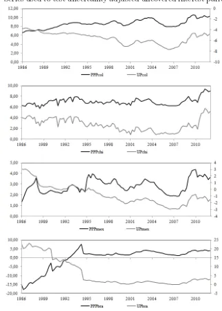
(idt −ift) = ∆set+1+σ(st−pdt +pft). (6) An important implication of UAUIP is that the expected change of the nominal exchange rates is not only related with the observed interest rate, but also with the interest rate differential corrected by the uncertainty premium. Figure (2) depicts,
pppdt condition, along withupt= ∆st+1−(idt−ift)for Colombia, Chile, Brazil and Mexico. According to IKE, the graphs should reflect a similar movement between these series.
such changes lead market participant to revise their forecast of the return and unit loss form holding open position.
Fluctuations in the equilibrium depend on new realizations of the causal variables and the exchange rate, and on how market participants revise their forecasting strategies.The equilibrium premium on foreign exchange and the market´s forecast of the future spot exchange rate can change in opposite directions between two consecutive time periods. The intuition behind this result is that a higher set+1, for example, creates an excess demand for foreign exchange, which bids up the exchange rate and creates a gain for bulls and a loss for bears; bulls lower their degree of loss aversion while it rises for bears. The resulting fall in the uncertainty premium for the bulls and rise for the bears leads to a lower equilibrium premium, UAUIP implies a large equilibrium premium when one side of the market, either the bulls or the bears, forecast a large potential unit loss from speculation while the other side does not.
In the model, forecast strategies of future price must change almost all the time; strategies that initially generate profits, sooner o later lose the ability to continue producing profits. That is the point that the REH approach ignores and at the same time constitutes the foundation of IKE. The swings away from PPP are related with these strategies, the swings occur because the market forecasting strategies of the exchange ratest+1 moves persistently away from PPP, causing the current exchange
rate to follow it.
A further difference between REH and IKE is that under REH a stationary real exchange rate is consistent with a stationary real interest rate differential, whereas under IKE equilibrium is defined as a stationary cointegration relation between the two. Indeed, when the real exchange rate is moving away from its benchmark value, the real interest rate differential has to move in a way that the equilibrium in the product market is restored, that is:
3
Brief literature review
Macroeconomic models of the REH are compatible with equilibrium in the goods market, a stationary real exchange rate and a stationary real interest rate differen-tial. However, some authors have suggested that PPP, UIP and the Fisher Parity condition may in fact be non-stationary; see for instance Frootet al. (1995), Rogoff (1996), Rogoffet al. (2008), Lopezet al. (2005), and Papellet al. (2006). Persistent deviations from the steady state are commonly known as puzzles or anomalies in the international macroeconomic literature and as such have been the topic of extensive research by several authors.
As an illustration, let us consider once again Figure 1 which presents the nominal exchange and the price relations of Colombia, Chile, Mexico and Brazil with respect to the price level in the United States. The systematic and persistent deviations between relative prices and the exchange rate are known in the literature as exchange rate swings. In order to explain such swings away from PPP, economists have constructed two types of monetary models, namely, those based on flexible prices and those based on sticky prices.
Flexible price monetary models assume that all prices including wages, adjust instantaneously to their equilibrium. In these models, deviations from PPP are caused by ’real disturbances’ to supplies. However long swings (as in Figure 1) require that such shifts be large enough, and in the same direction over several periods. But this behavior is not plausible in these models. Usually, in flexible-price models shifts occur in one direction in one period but in the opposite direction in the next one.
Literature about these anomalies or puzzles have been extensive. For example, Obstfeld and Rogoff (2000) indicate that it is likely that the pattern of exchange rate expectations lies behind many empirical puzzles found in international macroe-conomics. An idea that has been taken up under IKE by Frydman and Goldberg (2004, 2007, 2011), Frydman et al (2007) and Juselius (2009).
As indicated by Frydman and Goldberg (2004) There are two distinctive features of IKE. First, the authors develop an alternative framework for modeling forecasting behavior that recognizes that market participants posses only imperfect knowledge about the relationships driving asset prices. Second, the authors replace expected-utility theory with the prospect theory of Kahneman and Tversky (1979). Thus the authors build on prospect theory to model an idea due to Keynes (1936) according to which the risk in financial markets is connected to departures of asset prices from historical benchmark levels. As will be seen later, the uncertainly premium of the model depends on discrepancies between exchange rate and the relative prices.
Within this framework two major conclusions arise. First, swings away from parity can be based solely on macroeconomic fundamentals in contrast to the bubble view. Therefore policy makers can alter the course of macroeconomic fundamentals. Second, target zones and other intermediate exchange rate regimes may be effective even in situations in which policy institutions are not credible.
and Villamizar (2012) open the discussion about expectation of exchange rates by arguing that “the forward rate is generally different from the future spot rate, mainly because forecast errors are on average different from zero. This suggests that ex-change rate expectations are not rational” (pp.1), Ojeda (2009) provides evidence in favor of REH with unit root tests of PPP, but only after allowing for the presence of structural breaks. Also Ojeda,et al (2013) show evidence that fundamentals also play an important rate in the exchange rate dynamics at least for Colombia.
4
Empirical approach
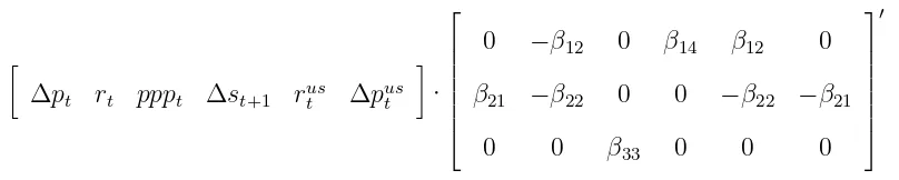
As indicated in the Introduction, the aim of the thesis is to apply the cointegration analysis through the formulation and estimation of a cointegrated vector autoregres-sive (CVAR) model to a data set of exchange rates and prices in four Latinamerican countries. In doing so, hypotheses derived from two fundamentally different ap-proaches will be tested. On the one hand, the REH implies that an agent can fully prespecify an economic model, leaving essentially no role for expectations. In this modeling approach an equilibrium in the good market is compatible with a station-ary real exchange and a stationstation-ary real interest rate differential. On the other hand, IKE implies that individual’s forecasting strategies play an important role in driving market outcomes. Because the individuals do not know the right model they have different forecasting strategies. It means that a speculative behavior is present in the model and when the real exchange moves away from its benchmark value (PPP), the real interest rate differential has to move in order to compensate and restore the product market.
(st−pdt+pft) ∆pdt ∆pft idt ift ∆st+1
′
.
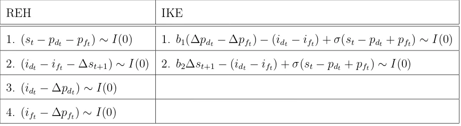
[image:13.595.85.545.269.395.2]The following table presents a summary of the cointegration relations that arise in both REH and IKE theoretical models:
Table 1. Cointegration relations
REH IKE
1. (st−pdt−pft)∼I(0) 1. b1(∆pdt −∆pft)−(idt −ift) +σ(st−pdt +pft)∼I(0) 2. (idt −ift −∆st+1)∼I(0) 2. b2∆st+1−(idt −ift) +σ(st−pdt+pft)∼I(0)
3. (idt −∆pdt)∼I(0) 4. (ift −∆pft)∼I(0)
One of the postulates of IKE is that when there is instability, that is when the market outcomes are away from their fundamentals, the individuals behave as postulated by the cointegration relations 1 and 2 of the IKE model (see Table 1). But also note that, ifst =pdt−pft, that is when the exchange rate is driving by its fundamentals, two things happen: First, the first cointegration relation of IKE is simply a lineal combination of relations 1, 3 and 4 of the REH model. Second, the second cointegration relation of REH is the same as the second cointegration relation of IKE. Thus, one can conclude that in those cases where individuals observe that outcomes are driven by fundamentals, there is no speculation and the REH holds.
4.1
Data
for all the variables needed to apply the CVAR-methodology. Therefore, the sample period to be considered for the four countries runs from 1986 to 2012.
Let d denotes Colombia, Chile, M exico and Brazil domestic countries, while the United States is the foreign one. The data consist of the following variables:
∆Pd= variation of consumer prices index for country d, ∆pd in logs.
∆Pus =variation of United States consumer prices index, ∆pus in logs.
id=the countryd loan rate.
ius =the Unites States loan rate.
S =the exchange rate of country d/ US, s in logs.
ppp = s−pd+pus the real exchange rate between country d and United State in logs.
Lower case letters denote variables in logarithms, with the exception of interest rates. All annual effective interest rate have been divided by 4 to achieve compara-bility between the quarterly inflation rates in log differences. Figure 3 presents the series used to build the models.
4.2
The estimated model
The following CVAR model is estimated for each country:
△xt= Πxt−1+ Γ1△xt−1+· · ·+ Γk−1△xt−k+1+µ+εt (8) Within the CVAR model, the cointegration hypothesis can be formulated as a reduced rank restriction on the Π matrix, also called the long-run matrix. If
xt ∼ I(1), then △xt ∼ I(0) implying that Π cannot have full rank. Therefore Π must have reduced rank, and so it can be decomposed as:
Π =αβ′,
where α is a p×r matrix that contains the adjustment coefficients, β is a p×r
endoge-nous variables in the VAR model, r ≤ p. µ denotes the deterministic components, and εt is the error term. The term β′xt−1 is an r×1 vector of stationary
cointe-gration relations. Then, all stochastic components are stationary in the model and equation (8) is consistent.
For each country, the CVAR model contains 6 variables: ∆pt, rt, pppt, ∆st+1, rust and ∆pus
t . Results not reported here suggest that rust and ∆pust can be regarded as exogenous variables, that is, they are variable that affect the other country-specific variables in the system, but are not affected by them. These results can be also justified based on economic intuition. Thus, in all models under consideration, both the United States inflation and interest rate are regarded as exogenous variables. Therefore the CVAR model contains,p= 4 endogenous variables, ∆pt, rt, pppt and
∆st+1; and 2 exogenous ones, rust and ∆pust .
Due to the regime changes in the Latinamerican’s exchange rate systems, struc-tural level breaks were also included in the vectors. In September 1999 the Colom-bia’s exchange rate band system was eliminated to allow a freely floating regime. Also Chile adopted inflation targeting scheme as well as flexible exchange rate sys-tem in Sepsys-tember 1999. In Mexico at the end of 1994 fixed exchange regime was eliminated. Finally, in January 1999 Brazil adopted a free exchange rate system. However, these level breaks were statistically significant in the cointegrated vector only for Colombia and Mexico. Additionally, due to the several changes in the fiscal and monetary policy in Brazil 1994, it was necessary introduce a break level vari-able in that period. For the four countries in the sample, there are 4 lags within the CVAR models and seasonal centered dummy variables. Lately, to improve the di-agnostic of the residuals, impulse dummy variables were incorporated in the models for Colombia and Mexico5
.
5
4.3
Rank determination
[image:16.595.98.494.559.773.2]Juselius (2006) argues that the determination of the cointegration rank may be a difficult choice. Indeed, the rank influences all subsequent inference and itself is a decisive step in the empirical analysis. However, macroeconomic theory gives insights about the rank of the Π matrix. The REH model postulates at least r=3 (PPP, UIP, FP and/or Interest rate differential), while IKE postulates r=2.
Table 3 presents the rank test for all countries in the sample,p−rare the common trends or pushing forces andrare the cointegration relations. Crucial results emerge from these results, essentially the rank ofΠ let us classify the four countries in two groups. Colombia and Chile form the first group with r=2, Mexico and Brazil, the second group with r=3. For the former group we can postulate that IKE describes better the macroeconomic outcomes, for the latter is the REH who better explains these outcomes. However, at this point it is premature to make these conclusions since we have not yet identified the cointegrated vectors.
4.4
Testing hypotheses on cointegration: REH or IKE?
This section identify the long-run structure by introducing restrictions on β′xt−1, The test tests whether the cointegrated vector is stationary, that is the null hypoth-esisβ′xt−1 ∼I(0).
Under r=2
• Model IKE1 :
∆pt rt pppt ∆st+1 rust ∆pust ·
0 β12 β13 β14 β15 0
β21 β22 β23 0 β24 β25
′
• Model IKE1∗:
∆pt rt pppt ∆st+1 rust ∆pust ·
0 −β12 β13 β14 β12 0
β21 −β22 β23 0 −β22 −β21
′
∆pt rt pppt ∆st+1 rust ∆pust ·
0 β12 0 β14 β15 0
β21 β22 0 0 β24 β25
′
• Model REH1∗:
∆pt rt pppt ∆st+1 rust ∆pust ·
0 −β12 0 β14 β12 0
β21 −β22 0 0 −β22 −β21
′
Note that the models with starsIKE1∗andREH1∗,have the same zero restrictions on beta that IKE1 and REH1, but also the first ones have a magnitude and sign
restrictions.
For both the IKE1 and IKE∗
1 we are testing the equilibrium conditions of the
IKE model (see Table 1). However, it is important to clarify that ifppptis stationary, then it is possible not reject the nule hypothesis of stationarity in the IKE model. However, this does not mean that IKE is the right model, this is because the sum of stationary variables is also stationary. So in that particular case the model is also compatible with the sum of stationary relations of the REH. Then REH could be the right model as well.
For that reason, although it makes not sense to test REH under r=2, because REH implies at least r=3. We present the casesβ13 =β23= 0, which are the cases whereIKE1 and IKE1∗ change toREH1 and REH1∗. In these cases we are testing
UIP and Interest rate differential, both equilibrium condition of REH model. Thus, ifREH1 and REH1∗ are not equilibrium relation butIKE1 andIKE1∗ are, in these
cases we can be sure that IKE is the right model because it’s clear that pppt is needed in the cointegrated vector.
Under r=3
• Model REH1:
∆pt rt pppt ∆st+1 rust ∆pust ·
0 β12 0 β14 β15 0
β21 β22 0 0 β24 β25
0 0 β33 0 0 0
• Model REH2∗:
∆pt rt pppt ∆st+1 rust ∆pust
·
0 −β12 0 β14 β12 0
β21 −β22 0 0 −β22 −β21
0 0 β33 0 0 0
[image:18.595.97.501.93.174.2] ′
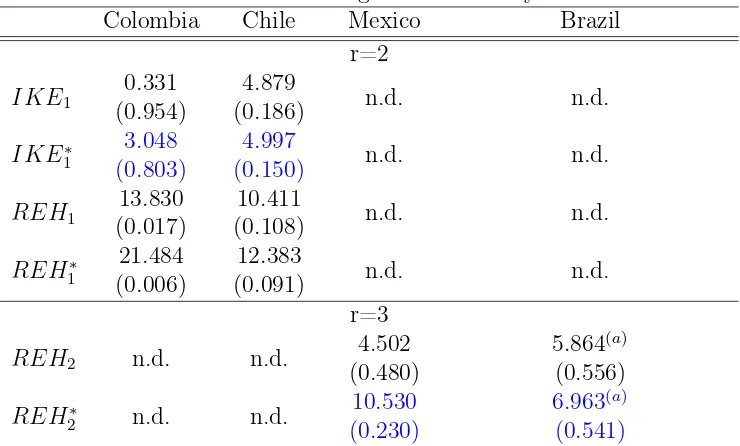
Table 4 presents the results of the χ2(v) tests of the cointegrated vectors. As we can see, Colombia is the strongest case where the IKE equilibrium relation cannot be rejected. Imposing the restrictions implied by model IKE1. Colombia has a
p−valueof 0.954 which is clearly not rejected. Also, thep−valueofIKE1∗ is 0.803 which is high. Note, that in the models REH1 and REH1∗, the nule hypotheses
of stationarity are rejected. Therefore, IKE appears to be the model which better describes the macroeconomic outcomes of Colombia over the sample period under consideration.
For Chile the results reported in Table 4 suggest that the equilibrium relation implied by IKE cannot be rejected. However, these results are not as stronger as those observed for the case of Colombia. Additionally, the p−value of the model
REH1 has ap−value of 0.10, a value near to the one of the IKE1∗. Therefore, we
opt for adopting the view of chile being a borderline case.
Regarding, Mexico and Brazil, these are countries in favor of the REH. Indeed, in both cases the cointegration analysis suggestsr= 3 and the equilibrium relations implied by REH are not rejected by the data either. However in Brazilpppt does not hold as an equilibrium, while the Fisher Parity condition, the interest rate differential and the UIP conditions were found to be stationary relations. For Mexico the the equilibrium relations of the REH model behave as stationary cointegrated vectors.
4.5
The cointegrated vectors
the β and α vectors for all countries. As can be seen, in all models the t−statitic
of the β vectors, presented in parentheses, are always higher than 1.96, Therefore, all variables are needed in the cointegrated vectors. Also, all the vectors have the correct sign postulated by the IKE and REH models.
In contrast to the REH model, one of the main implications of the IKE is that
pppt is not stationary by itself. Instead, other variables are needed to build a sta-tionary relation. Therefore, the inclusion of pppt in the IKE cointegrated vectors has a particular interest, since this variable should be always statistically significant,
pppt represents the uncertainty premium function, which is a function of the gap effectupt =σ(s−pdt+pft). In equation (6) we can seeupt implies that an increase in ∆se
t+1 will lead an excess of demand for the foreign exchange rate, where the
σ coefficient is related to the loss averse parameter. For Colombia and Chile this parameter is significant. Also, within each country the magnitude of the coefficient in the two cointegrated vectors is quite similar, between zero and one, as it was expected.
Although the cointegrated vectors of Mexico and Brazil are in favor of the REH, Mexico is the only country in which it is possible to find a lineal combination that makes pppt stationary by itself. These results are in line with the stationary test presented in table 66
. The test shows that Mexico is the only country wherepppt is a stationary relation.
A final test that shows the importance of theppptvariable in the IKE models, is the test of unit vector inalphapresented in Table 7. This test shows which variable are the pushing forces of the system and which are purely of adjusting (they only have transitory effects on the other variables). As we can see in the countries where IKE holds, pppt is presented as one of the pushing force of the system. Countries where REH holds the hypotheses of pppt as a pushing force is rejected.
6
5
Final considerations
Using a CVAR approach, we find that macroeconomic outcomes for Colombia and Chile appear to be better described by the IKE model, while REH seems to hold best for Mexico and Brazil. In the particular case of Colombia, in 2012 the Colombian peso was the most appreciated currency against the US dollar within a sample of 170 currencies. This thesis argues that such appreciation could have taken place because of speculative behavior of agents with imperfect knowledge regarding future payoffs. Therefore, it may well be the case that individuals are either not receiving the right signals from the market or that they do not have the right model to form their expectations.
According to the 2012 Financial Development Report of the World Economic Forum, Brazil is the country with the best financial stability indicator, followed by Chile, Mexico and Colombia. Therefore, one can conjecture that the more advanced the financial market, the more knowledge individuals will have about their markets. Thus, coutries with developed financial systems are more likely to be economies where the REH hold, while IKE appears more consistent with economies with less developed financial markets.
References
Arteaga, C., Granados, J., and Ojeda-Joya, J. (2012). “El comportamiento del tipo de cambio real en. Colombia: ¿Explicado por sus fundamentales?”. Borradores de Economía, Banco de la República.
Dornbusch, R. (1976a). “Exchange Rate Expectations and Monetary Policy,” Journal of International Economics, Vol. 6 (August), pp. 231–44
Dornbusch, R. (1976b). “Expectations and Exchange Rate Dynamics,” Journal of Political Economy, Vol. 84 (December), pp. 1161–76Echavarría, J. J., D.
(Jun., 1976), pp. 200-22
Fleming, M. (1962) “Domestic Financial Policies Under Fixed and Under Float-ing Exchange Rates,” Staff Papers, International Monetary Fund, Vol. 9 (Novem-ber), pp. 369–79
Frydman, R. and Goldberg, M. (2007) Imperfect Knowledge Economics: Ex-change rates and Risk. Princeton University Press
Frydman, R. and Goldberg, M. (2011) Beyond Mechanical Markets: Asset price swings, Risk and the Role of the State. Princeton University Press
Froot, Kenneth and Kenneth Rogoff (1995) “Perspectives on PPP and long-run real exchange rates,” in: G. Grossman and K. Rogoff, eds.,Handbook of International Economics III, Chapter 32.
Hayek, Nobel Prize lecture (1974)
Jongen, R., Willem F. C. and Christian C. P.(2008). “Foreign exchange rate expectations: survey and synthesis”,Journal of Economic Surveys 22(1), 140-65.
Johansen, Soren. (1988). “Statistics analysis of cointagrations vector,” Journal of Economic Dynamics and Control, Elsevier, vol 12(2-3). pagess 231-254.
Johansen, Soren (1997). “Mathematical and statistical Modelling of cointagra-tion,” Economics Working Papers, eco97/15, European University Institute.
Juselius, K (2006). The Cointagrated Var Model-Methodology and applications. Oxford University press
Juselius, K (2010). Testing the rational expectations hypothesis against the im-perfect knowledge hypothesis in a model for foreign exchange: A Scenario Analysis. Juselius, K (2011). “Imperfect Knowledge, Asset Price Swings and Structurals Slumps: A Cointagrated VAR Analysis of Their Interdependence”. Discussion Paper No. 10-31. University of Copehagen, Dept. of Economics.
Keynes, J. (1936). The General Theory of Employment, Interest and Money (London: Macmillan & Co.).
Kaltenbrunner, A. and Nissanke, M. (2009). “The Case for an Intermediate Exchange Rate Regime with Endogenising Market Structures and Capital Mobility: An Empirical Study of Brazil”. UNU/WIDER Research Paper. RP 2009-29.
Lopez, C., C. Murray and D. Papell. (2005). “State of the Art Unit Root Tests and Purchasing Power Parity,” Journal of Money, Credit and Banking, 37(2), pp. 361-369.
Mundell, R. 1963. "Inflation and Real Interest," Journal of Political Economy, University of Chicago Press, vol. 71, pages 280.
Obsfeld, M. and Rogoff, K. (2000) 2000b, “The Six Major Puzzles in International Macroeconomics: Is There a Common Cause?” in NBER Macroeconomics Annual 2000, ed. by Ben S. Bernanke and Kenneth Rogoff (Cambridge, Massachusetts:
MIT Press).
Ojeda, J. (2009). “Purchasing Power Prity and Breaking Tren Functions in the Real exchange Rate”. Borradores de Economía, Num. 564. Banco de la República. Otero, J. and Ramirez, M. (2006). “Inflation before and after Central Bank Independence: The Case of Colombia”. Journal of Development Economics. 79 (1) pp. 168-182.
Papell, D. and R. Prodan. (2006). “Additional Evidence of Long Run Purchasing Power Parity with Restricted Structural Change,” Journal of Money, Credit and Banking. 38 (5), pp. 1129-1349.
Pesaran, M. H., (1987) The Limits to Rational Expectations, Brasil Blackwell, Oxford
Rogoff, K. (1996). “The Purchasing Power Parity Puzzle,” Journal of Economic Literature, 34(2), pp. 647-668
Rogoff, K. and V. Stavrakeva (2008). “The Continuing Puzzle of Short Horizon Exchange Rate Forecasting,” NBER Working Papers, #14701
Solow, R. (1956). “A Contribution to the Theory of Economic Growth”, The Quarterly Journal of Economics, Vol. 70, No. 1. (Feb., 1956), pp. 65-94.
Paridad Cubierta y No Cubierta en Colombia 2000-2007", Ensayos Sobre Política Económica, v.26-56, pp.150-204.
Figure 3: Time series used to the CVAR model
Colombia
Exchange rates in logs Inflation Interest rate
Chile
Exchange rates in logs Inflation Interest rate
M exico
Exchange rates in logs Inflation Interest rate
Brazil
Table 2. Augmented Dickey-Fuller Test Equation for pppt
Colombia Chile M exico Brazil
t−satistics -0.421 -2.035 -3.131 -2.036
P rob 0.9004 0.2716 0.027 0.2710
Observations 102 102 102 102
Table 3: Rank trace tests
p−r r Colombia Chile M exico Brazil
4 0 97.335
(0.000)
121.919 (0.000)
129.723 (0.000)
118.740 (0.000)
3 1 57.924
(0.03)
46.507 (0.081)
77.608 (0.000)
79.172 (0.000)
2 2 27.596
(0.26)
20.650 (0.402)
42.162 (0.010)
43.151 (0.006)
1 3 5.676
(0.87)
2.630 (0.964)
6.929 (0.759)
11.040 (0.359)
Note: Structural change and dummy variables are included in the test. Therefore, test andp−valuein parentheses are generated using the simulation techniques
Table 4: Testing the stationarity
Colombia Chile Mexico Brazil
r=2
IKE1 0
.331 (0.954)
4.879
(0.186) n.d. n.d.
IKE∗
1
3.048 (0.803)
4.997
(0.150) n.d. n.d.
REH1 13
.830 (0.017)
10.411
(0.108) n.d. n.d.
REH1∗ 21.484
(0.006)
12.383
(0.091) n.d. n.d.
r=3
REH2 n.d. n.d. 4
.502 (0.480)
5.864(a)
(0.556)
REH∗
2 n.d. n.d.
10.530 (0.230)
6.963(a) (0.541) Note: p−valuesof theχ2(v)test in parentheses. Structural change and dummy
Table 5: αand β vectors
Colombia Chile Mexico Brazil
ˆ
β1IKE βˆ2IKE βˆ1IKE βˆ2IKE βˆ1REH βˆ2REH βˆ3REH βˆ1REH βˆ2REH βˆ3REH
∆pt 0.357 (3.549)
0 (n.a)
1.316 (16.687)
0 (n.a)
0 (n.a)
1.151 (32.157)
0 (n.a)
1.000 (n.a)
−1.000 (n.a)
0 (n.a)
rt
−1.000 (n.a)
−1.000 (n.a)
−1.000 (n.a)
−1.000 (n.a)
−1.000 (n.a)
−1.000 (n.a)
0 (n.a)
−0.064 (−9.876)
0.069 (9.708)
−0.048 (−8.130)
pppt
0.600 (9.970)
0.565 (16.124)
0.053 (2.039)
0.051 (2.053)
0 (n.a)
0 (n.a)
1.000 (n.a)
0 (n.a)
0 (n.a)
0 (n.a)
∆st+1 (n.a0 ) (70..521)417 (n.a0 ) (171.342.847) (291..068156) (n.a0 ) (n.a0 ) (n.a0 ) (n.a0 ) (n.a.1 )
rus t
1.000 (n.a)
1.000 (n.a)
1,000 (n.a)
1.000 (n.a)
1.000 (n.a)
1.000 (n.a)
0 (n.a)
0 (n.a)
−0.069 (−9.708)
0.048 (8.130)
∆pust −0.357 (−3.549)
0 (n.a)
−1.316 (−16.687)
0 (n.a)
0 (n.a)
−1.151 (−32.157)
0 (n.a)
0 (n.a.)
1.000 (n.a)
0 (n.a)
constant n.a. n.a. n.a. n.a. 0.008
(2.227)
0,008 (2,250)
−2.419 (122,107)
0 (n.a)
−6.056 (−21.942)
43.512 (17.014)
t99.q4 −3.586
(−8.738)
−3.434
(−13.450) n.a. n.a. n.a n.a. n.a. n.a.
0 (n.a)
0 (n.a)
t96.q3 n.a. n.a. n.a. n.a. (−−03..013664) (20..008250) (n.a0 ) n.a. n.a n.a
t94.q3 n.a. n.a. n.a. n.a. n.a. n.a. n.a. (n.a0 ) 5
.376
(17.367)
−44.019 (−15.337) ˆ
α1 αˆ2 αˆ1 αˆ2 αˆ1 αˆ2 αˆ3 αˆ1 αˆ2 αˆ3
∆pt
0.161 (0.706)
0.052 (0.260)
0.48 (1.029)
−0.337 (−1.626)
−0.155 (−0.656)
−0.602 (−2.533)
0.061 (4.437)
−2.337 (−1.273)
−2.188 (−1.232)
0.175 (0.963)
rt
0.102 (0.923)
0.314 (3.191)
0.740 (2.950)
−0.317 (−1.470)
−0.014 (−0.077)
−0.491 (−2.656)
0.018 (1.704)
258.903 (1.892)
233.728 (1.766)
15.872 (1.169)
pppt −0.050 (−4.451)
0.036 (3.603)
−0.019 (−2.377)
0.015 (2.263)
0.854 (1.967)
−1.147 (−2.624)
−0.060 (−2.387)
−0.023 (−1.825)
−0.021 (−1.750)
−0.001 (−0.581)
∆st+1
−1.524 (−0.931)
0.485 (0.334)
0.419 (0.371)
−1.182 (−1.216)
−3.191 (−3.547)
0.392 (0.434)
−0.092 (−1.775)
−6.121 (−2.418)
−6.361 (−2.599)
−0.936 (−3.727) Note: t−ratiosin parentheses.
Table 6: Test of stationarity
∆pt rt pppt ∆st+1
Colombia 9.970
(0.007)
2.416 (0.299)
18.679 (0.000)
4.991 (0.082)
Chile 1.135
(0.567)
4.687 (0.096)
21.103 (0.000)
1.308 (0.520)
Mexico 1.573
(0.210)
2.298 (0.130)
2.990 (0.084)
1.030 (0.164)
Brazil 6.184
(0.045)
6.494 (0.039)
25.586 (0.000)
Table 7: Test of Unit vector in alpha
∆pt rt pppt ∆st+1
Colombia 18.027
(0.000)
2.893 (0.235)
1.403 (0.496)
14.001 (0.001)
Chile 10.642
(0.005)
5.793 (0.055)
0.503 (0.778)
8.440 (0.015)
Mexico 3.639
(0.056)
17.572 (0.000)
4.626 (0.031)
1.228 (0.268)
Brazil 1.049
(0.306)
1.970 (0.160)
10.176 (0.001)
Table 8: Residual Analysis
Colombia(a) Chile M exico Brazil(b)
Test for autocorrelation
LM(1) ChiSqr(16) 4.537 [0.998] 24.698 [0.075] 27.882[0.173] 16.454 [0.422]
LM(2): ChiSqr(16) 3.604 [0.998] 4.908 [0.996] 16.519[0.672] 14.772 [0.541]
Test for Joint Normality ChiSqr(8) 18.597[0.017] 8.476 [0.388] 122.088 [0.000] 143.242 [0.000] Test for Normality
∆pt 3.253 [0.197] 2.756 [0.252] 14.480[0.001] 55.145 [0.057]
rt 7.133 [0.028] 5.267 [0.072] 61.049[0.000] 47.406 [0.000]
pppt 0.742 [0.690] 0.528 [0.768] 0.84 [0.657] 37.943 [0.000]
∆st+1 5.769 [0.055] 2.045 [0.360] 33.650[0.667] 18.673[0.000]
(a) with a dummy variable (dum99q2) is not possible reject the nule hypotheses of individual normality.
(b) with three dummy variables (dum 90q1. dum 89q3. dum99q) is not possible reject the nule hypotheses of individual normality.