Analysis of individual flows performance for delay sensitive applications

for Delay Sensitive Applications

Ricardo Nabhen1,2_{, Edgard Jamhour}2_{, Manoel C. Penna}2 _{and Mauro Fonseca}2 1 Laboratoire d’Informatique de Paris 6

Université Pierre et Marie Curie Paris – France

2 Pontifical Catholic University of Parana Curitiba – Parana – Brazil

{rcnabhen,jamhour,penna,mauro.fonseca}@ppgia.pucpr.br

Abstract. SLA management approaches typically adopt provisioning strategies based on aggregate traffic in order to support end-to-end delay requirements of applications. They do not take into account individual flows needs in terms of delay. However, this delay can be very higher than the one observed by aggregate traffic, causing an important impact in network application performance. This paper presents a study based on simulations that makes an analysis of the end-to-end delay observed by individual flows. Several scenarios are used to evaluate this performance and some metrics are proposed to investigate empirical relations that show the end-to-end delay behavior when are analyzed individual flows, the aggregate traffic and the network load.

1

Introduction

The necessity of quality of service (QoS) management in communication networks is unanimity, as well as the use of Service Level Agreements (SLA) for its implementation. The basis for quality evaluation is the specification of service level parameters which are jointly agreed by customers and service providers. Thus, a SLA establishes parameters and their levels that must be observed during service operation. Real time applications (e.g., voice over IP – VoIP and video-conferencing) and business critical applications are being considered in SLAs established between Internet Service Providers (ISPs) and their customers. In this context, a SLA specifies service level parameters, such as availability and mean time between failures, and network performance parameters, typically, delay, delay variation, packet loss rate and throughput [2].

architecture delegates a complex job to edge nodes, including tasks such as classification, marking, policing and shaping, making core network operation simpler[1].

Two approaches have been used for QoS management in DiffServ networks. The first one is based on the use of admission control mechanisms. The idea is to deny admission of new traffic that could cause degradation of the performance level experienced by current (i.e., previously admitted) traffic. Several admission control strategies have been proposed which can broadly be classified in two methods: centralized and distributed [3]. Centralized methods involve a central entity, named Bandwidth Broker (BB), which is responsible for admission control decisions. Proposals presented in [4], [5] and [6] are examples of centralized mechanisms. Conversely, proposals presented in [7] and [8] adopt the distributed method, where admission control decisions are taken by edge devices or end systems [9]. Regardless of the adopted method, the proposed mechanisms vary widely with respect to their implementation details. It is usual to find proposals based on new signaling protocols or based on schemes to measure network load using probing packets. A main difficulty of admission control approach is the complexity it introduces in QoS management. Thus, a second approach is being considered in order to simplify it, which is based on overprovisioning network resources. Roughly speaking, it consists in keeping such a network configuration that supports bandwidth requirements at network peak rate, which means to provision more resources than required to support the average load rate. A practical rule seems to guide overprovisioning process: Provisioning twice the capacity as the peak aggregate load[10]. By following this empirical rule, SLAs involving network performance parameters, including delay, jitter, packet loss rate and throughput would be assured.

Despite of the chosen approach we can identify difficulties when considering SLA assurance for delay sensitive applications. First, in the case of admission control mechanisms, we didn’t find any proposition that takes into account delay requirements. In fact, all revised mechanisms try to maximize bandwidth use, without considering the consequences on packet delay. Second, although the fundamental premise stated by overprovisioning approach, of keeping QoS management as simple as possible has a strong appeal, to restrict network traffic to fifty percent of network capacity can be an over simplification. In fact, under business perspective, service providers should try to maximize network resources use. Third, very few studies take into account individual flow requirements in order to handle fine-grained SLA involving delay parameters. As mentioned before, DiffServ operation is based on traffic aggregation, which renders management of individual flows performance a complex task. Finally, there certainly is a relationship between delay and network utilization level, but as far as we know, all studies just consider the mean percentage of bandwidth use, without considering its variation. We intend to explore the last two points in depth in our work.

commitments. Our concern is to consider deeply this issue, being able to answer more specific questions related to delay sensitive applications. For example, in a scenario that establishes a SLA where 97% of packets of each individual flow of a VoIP application in a DiffServ domain must observe a maximum end-to-end delay, we should be able to answer the following questions: Is it possible to guarantee this agreement just considering provisioning levels assigned to the aggregate traffic class? What is the relation between the aggregate traffic and its individual flows in terms of end-to-end delay? What are the main factors that affect individual flows performance in this context?

The use of bandwidth allocation in a per class basis for assuring QoS in DiffServ networks is a ubiquitous practice. The great majority of proposals limit the ratio of bandwidth allocation to assure quality for a given service class. However, there is no discussion about the time interval where this ratio should be computed. In our view, this is a fundamental issue if we want to control fine grain SLAs for delay sensitive application. In fact, unpredictable delay occurs due to packet queuing in IP routers, thus, and the mean bandwidth allocation can be acceptable, for example, when calculated in a daily basis, but unacceptable if during peak use intervals the network produces unacceptable packet delay.

In this paper we present a simulation-based study that analyses the end-to-end delay observed by individual flows of delay sensitive applications. It shows that this delay can vary widely in relation to the one observed in aggregate traffic. This variation must be considered when one establishes network provisioning levels. Also, some empirical evidences are investigated in order to show the relation between individual flows and aggregate traffic in terms of end-to-end delay, considering network utilization rate observed during the determined period of analysis. The paper is organized as follows. Section 2 reviews some related work. Section 3 presents our end-to-end delay analysis methodology for the study of individual flows performance. Section 4 presents the simulation results and their analysis. Finally, Section 5 summarizes the main aspects in this study and points to future work.

2

Related Work

In their seminal work, Fraleigh, Tobagi, and Diot have analyzed several backbone traffic measurements and have shown that the average traffic rate is much lower than link capacities (around 50%) suggesting that low utilization could be a strategy for network resources provisioning [11]. They have concluded that delay is not a relevant issue when dealing with aggregate traffic within high capacity backbones (above 1 Gbits/s), considering 50% of utilization level. Moreover, they showed that network utilization could reach 80% to 90% and delay values would remain acceptable for almost all applications. Their conclusions have influenced the overprovisioning approach to deal with delay requirements on IP networks. However, as said before, overprovisionig may be costly and sometimes impossible to be implemented. For example, leased-lines, wireless links and other access networks have typically low capacity, what renders the approach unfeasible.

end-to-end delay in aggregate class would be the same as those observed in each embedded individual flow. However, some studies show that end-to-end delay can vary sufficiently to produce service degradation. Jiang and Yao have investigated the impact of flow aggregation in end-to-end delay observed by individual flows in a DiffServ network [12]. This study considers a single aggregation traffic class and has evaluated multiple scenarios with the variation of network load and burstiness level. Results suggest that individual flow delay varies with respect to aggregate flow delay, according to bandwidth utilization level and the variation of the traffic burstiness level. A similar study realized by Siripongwutikorn and Banerjee has investigated individual flows delay embedded in a single traffic class, by considering the provisioning strategy based on aggregate traffic [13]. They considered several scheduling disciplines, such as FIFO and WFQ in their analysis, and the results indicate that traffic heterogeneity, network load and scheduling disciplines affect individual flows performance. Xu and Guérin have studied the performance of individual flows, in terms of packet loss rate, in a scenario where service level guarantees are offered to traffic classes [14]. They proposed an analytical model that measures the performance level of aggregate traffic, in order to foresee individual flows performance. Presented results show that when there are a great number of users it is desirable to avoid the aggregation of traffic flow with different profiles. They also evaluated what additional resources are necessary in order to reach the established loss rate assigned to individual flows.

Our work differs from above studies in several points. First, in the same way as previous studies, we relate delay analysis to network utilization rate, but differently we consider the variation of network utilization rate during simulation time. We show that it is important to consider variation of network utilization rate when evaluating individual flows delay. The second difference is the evaluation metrics. Xu and Guérin study does not consider delay but packet loss rate. Siripongwutikorn and Banerjee

analyses the delay of the 99th

percentile of packets of individual flows, while our work

considers the 97th

percentile, the one usually adopted as a reference for good quality

voice flows1_{. Moreover, we propose the use of a new metric to evaluate the effects of}

the network load variation in the delay of individual flows. Beside of these differences, our work also brings a contribution by explicitly handling VoIP flows. We analyze two scenarios, the first handling just concurrent VoIP flows and the second handling concurrent VoIP flows mixed to data traffic. In summary, our work proposes new metrics to investigate the relation between end-to-end delays observed in individual flows with respect to that observed in the aggregate flow, by taking into account the probability distribution of network utilization rate computed for specific time intervals.

3

End-to-end Delay Analysis Methodology

3.1 Delay Requirements and Simulation Hypothesis

Real time applications have typically their SLAs specified in terms of end-to-end delay bounds with deterministic or probabilistic guarantees [11]. In the former case, one hard delay limit is defined,

while, in the latter case, delay limits are associated to percentiles

of delivered packets, as can be seen in Table 1. When using deterministic guarantee, every delivered packet should experience at most 50ms end-to-end delay, whereas in the

probabilistic guarantee case, 97%of delivered packets should experience at most 50ms

end-to-end delay and 99%should experience not more than 60ms.

Table 1. End-to-end delay guarantees example

Network delay is a function of several sources: (i) Transmission delay: time to transmit a packet on a link; (ii) Queueing delay: time spent in node buffers waiting for service; (iii) Propagation delay: time related to physical media and link extension; (iv) Processing delay: time related to the switching process. The end-to-end delay observed by a packet is affected differently by each delay source. For example, for low capacity links and depending on packet lengths transmission delay could be relevant but it is negligible for high capacity ones. Propagation delay should be considered only in long distance links (e.g., continental links). Processing delay is negligible for the majority of recent network devices. Finally, queuing is the most challenging delay source for researchers and network engineers because of its dependence to traffic behavior, due to the difficulty of developing analytical models that renders the arrival processes non predictable.

Delay requirements for voice applications are well known. For example, ITU-T states that real time applications will not be affected by end-to-end delay lower than 150ms [15]. This value can be used as a deterministic limit for high quality flows. Actually, a sufficient condition for considering a VoIP flow as a high quality one is 97% of delivered packets to observe an end-to-end delay lower than 150ms [15]. However, the choice of appropriate provisioning levels to assure fine grain SLAs involving end-to-end delay in IP networks remains as a major challenge. A simple and usual solution is overprovisioning, but as mentioned before, it may be costly and sometimes impossible to be implemented.

From previous analysis of provisioning strategies two questions remain unanswered: (i) Is it possible to guarantee service level agreements based on probabilistic guarantees for individual flows of delay sensitive applications by considering provisioning levels assigned to aggregate traffic classes? (ii) How is individual flows end-to-end delay affected by variation of network utilization rate, especially during periods of higher network utilization rates? To answer these questions we performed simulations using

Deterministic Guarantee

Probabilistic Guarantee

50ms 97,0% - 50ms

the Network Simulator version 2 (NS-2) to observe end-to-end delay behavior of individual flows considering several network load conditions in order to obtain the relation between individual flow to-end delay with respect to aggregate traffic end-to-end delay.

3.2 Topology and Stages of Simulation

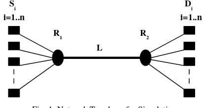
Fig. 1 shows the network topology adopted in simulation. Several traffic pairs (Si,Di)

were instantiated, where each pair generates only one VoIP flow during simulation period. Every generated flow is analyzed in order to evaluate the end-to-end delay of its

packets. In fact, the highest end-to-end delay observed within the 97th

percentile is recorded to compute the performance metrics (see section 3.4). Bandwidth of link L is set to 2 Mbps, because high network utilization rates should be reached. This would be difficult to achieve with higher capacity links, due to low throughput required by each individual VoIP flow (around 30kbps). Propagation delay was not considered as well as processing time at codecs. Although both delay sources must be considered in the overall performance evaluation of a VoIP flow, in the context of this work, which focus is on the analysis of the individual flows performance in terms of delay taking into account variation of network utilization rate, the conclusions would be not modified by

those fixed values (i.e., propagation and codec delays). Buffers of routers R1 and R2

were adjusted in order to avoid packet loss because its occurrence would affect the determination of target packets for delay analysis and we are just interested in delay analisys of delivered packets.

Fig. 1. Network Topology for Simulation

In order to get a more precise analysis the simulation was organized in two stages: stage 1, involving just VoIP traffic and stage 2, involving mixed VoIP and data traffic. They were defined because the distribution of the network utilization rate observed during simulation period has shown distinct behavior when mixed traffic was introduced, as shall see in Section 4. Stage 1 can be seen as a scenario where one queue is used to serve all aggregate traffic formed by VoIP flows. Here we intend to analyze the influence of DiffServ aggregation strategy in the performance of individual VoIP flow, with respect to end-to-end delay. On the other hand, Stage 2 can be seen as a scenario where voice traffic is mixed with data traffic with no service differentiation. Here we want to see how data traffic would interfere with VoIP flows.

3.3 Traffic Source Parameters

S i i=1..n

R 1

D i i=1..n

R 2

VoIP applications usually are simulated as a constant bit rate flow. Depending on the codec, traffic may vary widely. For example, G.711 codec requires higher bandwidth than other codecs, however, it provides the best mean opinion score (MOS) [15], a numerical metric that indicates the quality of human speech in a voice circuit. Silence suppression is an important feature to reduce the required bandwidth for VoIP applications. In this case, we have used the same traffic model adopted in [16], where talk-spurts and silence gaps are both exponentially distributed with the mean equals to 1.5 seconds. Also, the VoIP packet size (payload and headers) is 74 bytes and during transmission periods the packet interarrival time is 20 milliseconds. A major issue in our simulation is the traffic intensity generated by concurrent VoIP flows. In this case, based on the study presented in [17] we use two traffic parameters: the average flow duration (AFD) that establishes an average value in seconds for the duration of a VoIP flow; and the time between flows (TBF) that establishes an average value in seconds for the flow arrival process. AFD and TBF are both exponentially distributed according to the specified mean.

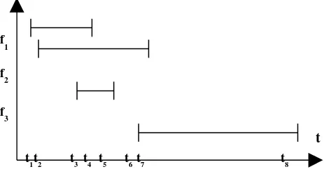
Fig. 2 illustrates the VoIP flows generation process. It shows four VoIP flows

starting at instants t1, t2, t3 and t6, respectively, representing the exponential distribution

of the TBF parameter. VoIP flows have different duration times, due to exponential

distribution of the AFD parameter. The duration time of flows f1 and f4 have are

respectively given by t4-t1 and t8-t6. For data traffic, we have adopted a combined traffic

model based on the Internet distribution packet size presented in [18]. It is composed by 58% of 40-byte packets, 33% of 552-byte packets and 9% of 1500-byte packets. In terms of simulation, the Pareto distribution was used to implement this traffic source considering the ON and OFF parameters, respectively, 500ms and 125ms. The shape parameter adopted was 1.5 as suggested in [19].

Fig. 2. VoIP flows: Generation process example

3.4 Simulation Scenarios

Simulation time was set to 400s because of the average duration of each VoIP flow and its arrival process, as can be seen in the AFD and TBF parameters in Tables 2 and 3. In this case, this simulation time permits an adequate period for the proposed analysis methodology since a value of 210s for the AFD parameter and a value of 3.5s for the TBF parameter allow the observation of several concurrent VoIP flows during this simulation time. This approach allows clearly the simulation of the arrival and termination processes of VoIP flows usually observed in real scenarios. As presented

t

t

1t2 t3 t4 t5 t6 t7 t8 f

1

f

2

f

3

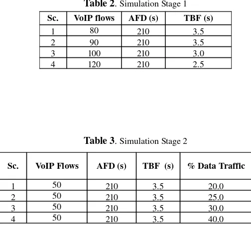
in section 3.2, simulation scenarios are divided into two stages. Tables 2 and 3 show, respectively, the configuration of each scenario in each stage.

Table 2. Simulation Stage 1

Table 3. Simulation Stage 2

The TBF parameter in stage 1 (see Table 2) was decreased in order to generate higher load conditions; a lower TBF represents a lower average time between flows, thus, increasing the number of VoIP flows during a specific time. Four scenarios have been simulated in each stage. In Stage 1, the number of concurrent VoIP flow increases at each new scenario, in order to increase network load. In Stage 2, the number of concurrent VoIP flows is kept constant, but the data traffic rate increases at each new scenario.

3.5 Performance metrics

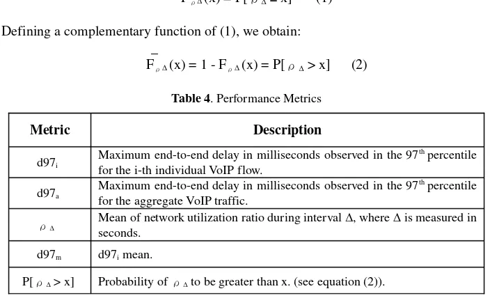
In order to investigate the relation between end-to-end delays observed in individual flows with respect to that observed in aggregate traffic we define some performance metrics, as shown in Table 4, which were analyzed under several simulation scenarios. These metrics will be used to investigate empirical relations between network load and delay of individual flows. Delay performance for individual flows and aggregate traffic

can be verified by inspecting d97i and d97a. The d97i and σ97 metrics are analyzed

with respect to the variation of the ρΔmetric, i.e., its probability density function

Sc. VoIP flows AFD (s) TBF (s)

1 80 210 3.5

2 90 210 3.5

3 100 210 3.0

4 120 210 2.5

Sc. VoIP Flows AFD (s) TBF (s) % Data Traffic

1 50 210 3.5 20.0

2 50 210 3.5 25.0

3 50 210 3.5 30.0

(pdf), in order to seek a possible empirical relation between aggregate traffic, individual flows and the distribution of the network utilization rate. In this context, a cumulative

distribution function (cdf) of ρ_∆ is calculated by the integral of pdf(ρ∆) and can be

denoted as follows:

Fρ∆(x) = P[ρ∆ ≤ x] (1)

Defining a complementary function of (1), we obtain: _

Fρ∆(x) = 1 - Fρ∆(x) = P[ρ∆ > x] (2)

Table 4. Performance Metrics

Metric Description

d97i

Maximum end-to-end delay in milliseconds observed in the 97th

percentile for the i-th individual VoIP flow.

d97a

Maximum end-to-end delay in milliseconds observed in the 97th _percentile for the aggregate VoIP traffic.

ρ∆ Mean of network utilization ratio during interval ∆, where ∆ is measured in

seconds. d97m d97i mean.

P[ρ∆ > x] Probability of ρ∆ to be greater than x. (see equation (2)).

4

Simulation Results and Analysis

4.1 Stage 1: VoIP Traffic

Mean of network utilization ratio during interval ∆ (ρ∆) is a major parameter in

simulation and it is obtained as follows: simulation is repeated 20 times for each scenario and we compute the network load given by the input traffic due to the

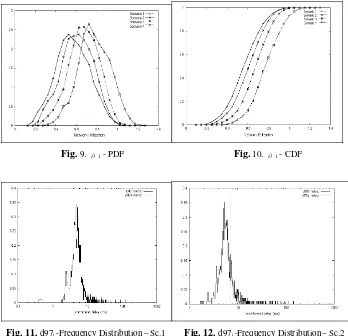
aggregation of independent VoIP sources in intervals defined by ∆. Figs. 3 and 4 show,

respectively, the probability density function and the cumulative distribution function

with normalized values for the ρ1 metric observed during stage 1. These graphs

represent the results given by all simulations. End-to-end delay values shown later in this section will be presented along with their 95% confidence intervals.

One of the main issues to be investigated in this work is the delay experienced by packets under different load conditions and, mainly, how their variation affect this

delay. Observing the average network load during the simulation period, i.e., ρ400, in

scenarios 1, 2, 3 and 4, respectively, 40.74%, 50.21%, 55.58% and 64.86%, and considering the overprovisioning rule, these values were supposed to be adequate for supporting delay sensitive applications. However, in all scenarios, we can observe the

network utilization rate given by ρ1 above 90%, which could affect considerably the

end-to-end delay of individual VoIP flows2_{. In fact, when computed for smaller}

intervals (Δ), ρ∆ reaches unacceptable values which sometimes could represent a SLA

violation. From Fig. 4, for example, one can observe that the probability of ρ1 to be

higher than 90% is, respectively, 0.41%, 2.28%, 7.02% and 20.00% for scenarios 1, 2, 3 and 4. We can conclude that it is meaningless to discuss the mean of network utilization

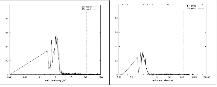
rate without taking into account the interval in which it is computed (∆). Figs. 5, 6, 7

and 8 show the frequency distribution (normalized values) of d97i for scenarios 1, 2, 3

and 4, where end-to-end delay axis has been plotted on a logarithmic scale. d97i is

computed by considering all values registered in all simulation repetitions, that is, 1600, 1800, 2000 and 2400 VoIP flows for scenarios 1, 2, 3 and 4. The vertical line in each

graphic depicts the maximum end-to-end delay observed in the 97thpercentile for the

aggregate VoIP traffic (d97a). In all scenarios we can see several VoIP flows where d97i

is greater than the d97a. This result can be justified by the strategy of grouping all

packets of every individual flow in order to compute the 97th

percentile of the aggregate

traffic. In this context, it is important to mention that either d97a or d97i are computed

using the same data set. Using this grouping scheme, it is clear that the 97th

percentile

of the aggregate traffic is below the 97th

percentile of some individual flows (i.e., flows

that ocurred during higher load conditions) and, therefore, their d97i are expected to be

higher than the associated d97a.

Fig. 3. ρ1 - PDF Fig. 4. ρ1 - CDF

Fig. 7. d97i -Frequency Distribution– Sc.3 Fig. 8. d97i -Frequency Distribution– Sc.4

4.2 Stage 2: Mixed VoIP and Data Traffic

The difference between stage 1 and stage 2 is that we have mixed data traffic with VoIP flows to generate background traffic. We calculated the same performance metrics, only

for packets of VoIP flows. Figs. 9 and 10 show the normalized values for ρ1 frequency

distribution observed during stage 2. Here we can observe higher average network

utilization rates than those observed in stage 1. The calculated values for ρ400 (Δ=

simulation time) in scenarios 1, 2, 3 and 4 are 55.65%, 61.12%, 64.87% and 75.29%, respectively. However, when comparing Figs. 4 and 10, we observe more instances of

higher values of ρ1 in stage 1 than in stage 2. This explains the better results even

under higher average network utilization rates observed in stage 2.

Figs. 9, 10, 11 and 12 show the frequency distribution of the d97i for scenarios 1, 2,

3 and 4 as explained before. As in stage 1, in all scenarios we can see several VoIP

Fig. 9. ρ1 - PDF Fig. 10. ρ1 - CDF

Fig. 11. d97i -Frequency Distribution– Sc.1 Fig. 12. d97i -Frequency Distribution– Sc.2

4.3 Remarks

Tables 5 and 6 present the computed values for d97m and σ97 metrics in each scenario,

along with their 95% confidence intervals. Also, the corresponding values of P[ρ1 >

100%] and ρ400 are presented. For scenarios 1 and 2 of both stages the P[ρ1 > 100%]

is almost negligible. As can be seen, the end-to-end delay remains very steady under

these load conditions. In addition, due to the similar value of P[ρ1 > 100%], the

scenario 3 in Table 6 also showed an acceptable performance in terms of the d97m

metric and its variability (i.e., the σ97 metric). This behavior cannot be seen in

scenario 3 in Table 5, where a slightly increase of P[ρ1 > 100%] (i.e., to 2.39%)

caused a sensible variation of the d97m and σ97 metrics. Finally, the scenario 4 of

both stages experienced a significant increase of the network utilization rate, easily

noted in the values of P[ρ1 > 100%] in Tables 5 and 6, causing exponential augment of

the d97i and σ97 metrics to prohibitive levels.

Table 5. Stage 1: d97m _; σ97 ; _P[ρ1 > 100%] metrics

Table 6. Stage 2: d97m _; σ97 ; _P[ρ1 > 100%] metrics

It is important to examine the values in Tables 5 and 6 in light of the frequency

distribution of the ρΔ. For example, ρ400 is 64.86% in scenario 4 of stage 1 and

75.29% in scenario 4 of stage 2, but d97m was twice higher in the former case which can

Sc. d97m Confidence

Interval (95%) σ97 P[ρ1 > 100%] ρ400

1 1.46 [1.27 ; 1.64] 3.48 0.31% 40.74%

2 3.90 [3.40 ; 4.39] 9.78 0.97% 50.21%

3 81.50 [73.00 ; 89.99] 176.46 2.39% 55.58%

4 1000.84 [903.57 ; 1098.10] 2202.51 9.82% 64.86%

Sc. d97m Confidence

Interval (95%) σ97 P[ρ1 > 100%] ρ400

1 7.11 [6.43 ; 7.80] 10.05 0.56% 55.65%

2 8.64 [7.82 ; 9.46] 12.06 1.06% 61.12%

3 16.63 [14.93 ; 18.33] 24.86 1.23% 64.87%

be explained by the PDF of ρ∆. It is clear from the analysis of Figures 3 and 9 that in stage 1 (see Figure 3) the system remains under higher load conditions which affects

directly the overall delay performance given by d97m and σ97 metrics, regardless of

the fact that the value of ρ400 could indicate the contrary. On the other side, in the

scenarios under lower network utilization, this anomaly does not verify, what clearly indicates the importance of considering the network utilization distribution in the context of individual flows performance.

5 Conclusion

This paper presented a study in order to investigate the end-to-end delay behavior observed by individual flows. It is important to understand this behavior and its relation with aggregate traffic and network utilization, mainly when one considers the SLA management for delay sensitive applications. In order to perform this analysis, this study has considered delay requirements for VoIP applications, which defines a

maximum end-to-end delay to be experienced by the 97th _{percentile of packets from}

each individual VoIP flow. New metrics were defined to evaluate empirical relations between network load and delay of individual flows. Empirical relations were established by an extensive two stage simulation experiment, with multiple scenarios simulating several traffic configurations and a multiplicity of load conditions.

Results confirmed that network utilization ratio is one the parameters that affect the most the delay in IP networks. Moreover, the study presented a new approach to relate network load with delay. It is shown that it is meaningless to consider the mean of network utilization rate without taking into account the interval in which it is computed. Analyzed scenarios indicate that even when the average network utilization rate observed is acceptable, for example under overprovisioning empirical rules, the delay performance observed by several individual flows is impracticable. This new approach suggests that any statement about network utilization rate should also state the time interval in which it is computed, mainly when one considers the SLA specification based on individual flows performance metrics.

References

1. S. Blake, D. Black, M. Carlson, E. Davies, Z. Wang, and W. Weiss, RFC

2475: An architecture for differentiated service. IETF (1998).

2. A. Westerinen, J. Schnizlein, J. Strassner, M. Scherling, B. Quinn, S. Herzog,

A. Huynh, M. Carlson, J. Perry, and S. Waldbusser, RFC 3198: Terminology for policy-based management. IETF (2001).

3. W. Rhee, J. Lee, J. Yu, and S. Kim, Scalable quasi-dynamic-provisioning

based admission control mechanism in differentiated service networks. ETRI Journal, 26(1):22–37 (2004).

4. R. Liao and A. Campbell, Dynamic core provisioning for quantitative

5. Z. Zhang, D. Zhenhai, and Y. Hou, On scalable design of bandwidth brokers. EICE Transactions on Communications, e84-b(8) (2001).

6. C. Bouras and K. Stamos, An adaptive admission control algorithm for

bandwidth brokers. Third IEEE International Symposium on Network Computing and Applications(NCA) (2004).

7. V. Elek, G. Karlsson and R. Ronngren, Admission control based on end-to-end

measurements. IEEE INFOCOM (2000).

8. L. Breslau, S. Jamin and S. Shenker, Measurement-based admission control:

What is the research agenda? IEEE IWQoS (1999).

9. F. Kelly, P. Key and S. Zachary, Distributed admission control. IEEE Journal

on Selected Areas in Communications, 18:2617–2628(2000).

10. C. Filsfils and J. Evans, Deploying diffserv in backbone networks for tight sla control. IEEE Internet Computing Magazine(2005).

11. C. Fraleigh, F. Tobagi, and C. Diot, Provisioning ip backbone networks to support latency sensitive traffic. The 22nd Annual Joint Conference of the IEEE Computer and Communications Societies, Infocom(2003).

12. Y. Jiang and Q. Yao, Impact of fifo aggregation on delay performance of a differentiated services network. The International Conference on Information Networking, ICOIN (2003).

13. P. Siripongwutikorn and S. Banerjee, Per-flow delay performance in traffic aggregates, Proceedings of IEEE Globecom(2002).

14. Y. Xu and R. Guérin, Individual Qos versus Aggregate Qos: A loss performance study. IEEE/ACM Transactions on Networking, 13:370– 383(2005).

15. ITU-T (2003). Recommendation g.114: One-way transmission time. ITU-T.

16. C. Boutremans, G. Iannaccone and C. Diot, Impact of link failures on voip performance. Proceedings of NOSSDAV Workshop (ACM Press) (2002).

17. Cisco. Traffic analysis for Voice over Ip. Cisco Document Server (2001).

18. K. Claffy, G. Miller and K. Thompson, The nature of the beast: Recent traffic measurements from an internet backbone. Proceedings of INET’98 (1998).

19. C. Dovrolis, D. Stiliadis and P. Ramanathan, Proportional Differentiated