Characterization of the agent causing a new disease in leek (Allium ampeloprasum var borrum) fields by RNA Seq

Texto completo

(1)Characterization of the agent causing a new disease in leek (Allium ampeloprasum varborrum) fields by RNA-Seq Ana Ruiz Padilla Máster en Bioinformática y Bioestadística Análisis de datos ómicos María Ángeles Ayllón Talavera Guillem Ylla January 2nd 2019.

(2) Esta obra está sujeta a una licencia de Reconocimiento-NoComercialSinObraDerivada 3.0 España de Creative Commons.

(3) FICHA DEL TRABAJO FINAL. Título del trabajo:. Characterization of the agent causing a new disease in leek (Allium ampeloprasum varborrum) fields by RNA-Seq. Nombre del autor:. Ana Ruiz Padilla. Nombre del consultor/a:. Guillem Ylla Bou. Tutor externo. María Ángeles Ayllón Talavera. Nombre del PRA:. David Merino Arranz. Fecha de entrega (mm/aaaa):. 01/2019. Titulación:. Máster en Bioinformática y Bioestadística. Área del Trabajo Final:. Análisis de datos ómicos – Proyecto Fin de Máster. Idioma del trabajo:. Inglés. Palabras clave. RNAseq, leek, virus. Resumen del trabajo En 2011, se describió una nueva enfermedad, llamada en este informe enfermedad emergente en puerro (EEP), en campos de puerro de Segovia. La enfermedad estaba caracterizada por anormalidades en el desarrollo, como geotropismo y deformación de las raíces; y decoloración de bulbos y hojas. Se desconoce la etiología de la enfermedad, pero los síntomas podrían estar asociados a la infección por diferentes patógenos que se distribuyen de forma sistémica en las plantas como virus y fitoplasmas. Con el objetivo de identificar los patógenos causantes de la EEP, se tomaron muestras de hojas y se extrajo el ARN total de estas. A su vez, se realizó el mismo proceso con plantas sanas. A partir de estos extractos, se realizaron 4 mezclas con RNA de plantas enfermas (Sick1, Sick2, Sick3 and Sick4) y una mezcla con RNA de plantas sanas (Control2) que fueron enviadas a secuenciar. Los datos resultantes de la secuenciación fueron analizados con el objetivo de identificar los microorganismos patógenos causantes de la enfermedad. Este análisis bioinformático incluía distintos pasos. Los más relevantes fueron el control de calidad de las secuencias originales, la eliminación de adaptadores y la selección de lecturas presentes exclusivamente en las mezclas de plantas enfermas. Se seleccionaron aleatoriamente el 10% de los “contigs” de cada pool para evitar problemas de falta de recursos computacionales.. i.

(4) Finalmente, las secuencias de interés fueron analizadas para identificar los posibles patógenos presentes. Los resultados mostraron la presencia de fitoplasmas y otros microorganismos como posibles causantes de la enfermedad. Abstract: A new disease, in this report called emergent disease in leeks (EDL), that affects leek (Allium ampeloprasum var. porrum) fields was discovered in the Segovia in 2011. This EDL is characterized by the development of abnormalities, which includes root geotropism and deformation, and leaves and bulb discoloration. The etiology of the disease is currently unknown, but the symptoms are associated with the infection of systemic biotrophic pathogens like viruses and phytoplasmas. With the goal of identifying pathogens causing EDL, total RNA was extracted from leaves of healthy leek plants grown in a greenhouse facility and infected plants showing symptoms of the disease. Five pools were prepared by mixing total RNA: four from infected ones (Sick1, Sick2, Sick3 and Sick4) and one from control samples pool C- (Control) that were sent for sequencing. We analysed the NGS data to identify the microorganisms associated with diseased leek plants. The most important steps of this analysis were: control of the quality of raw reads, trimming the adapter sequences and selection of the contigs present in the infected pools and not in the healthy ones. We took only a sample of 10 percent of the selected contigs to avoid problems with lack of computational resources. Finally, the sequences of interest were analyzed to identify the possible pathogens present. The results showed the presence of phytoplasm and other microorganisms as possible pathogens associated to the disease.. ii.

(5) Index 1. Introduction .................................................................................................. 1 1.1 Context and project justification ............................................................ 1 1.2 Objectives of the project ......................................................................... 3 1.4 Planning ................................................................................................... 5 1.5 Short summary of obtained products.................................................... 6 1.6 Short description of chapters of the memory. ...................................... 7 2. Chapters ........................................................................................................ 8 2.1. Computing environment preparation ................................................... 8 2.2. Data acquisition and familiarization ..................................................... 8 2.3. FastQC quality control analysis before and after trimming. ............... 9 2.4. Trimming of adapters with Trimmomatic ........................................... 16 2.5. Assembly de novo of reference transcriptome using Trinity ........... 17 2.6. Mapping against the new created transcriptome with Bowtie2. ...... 20 2.7. Table of counts generation and selection of transcripts of interest.21 2.8. Results .................................................................................................. 22 3. Conclusions ................................................................................................ 25 4. Glossary ...................................................................................................... 26 5. Bibliography ............................................................................................... 27 6. Annexes ...................................................................................................... 29 6.1. Commands applied in Ubuntu bash for the installation and running of the programs. .............................................................................................. 29 6.2. Graphics obtained in FastQC reports ................................................. 36 6.3. Table of plant pathogenic organisms present in diseased pools .... 48. iii.

(6) Figures list Figure 1. Scheme of basic steps of the RNA-seq process Figure 2. Scheme of pools preparation Figure 3. Workflow followed in the final master project Figure 4. Gantt diagram showing the planning followed for the final project master Figure 5. Table of main characteristics of files and new names assigned to work with them Figure 6. Summary table of main characteristics of FastQC files Figure 7. Sequence length distribution graphics for samples Control_1 and Sick1_1 Figure 8. Quality score graphics of samples Control_1 and Sick1_1 before and after trimming Figure 9. Per tile sequence quality graphics of samples Control_1 and Sick1_1 before and after trimming Figure 10. Per sequence quality scores graphics of samples Control_1 and Sick1_1 Figure 11. Adapter content of samples Control and Sick1 Figure 12. Other graphs included in the report of Control_1 Figure 13. Steps of palindrome mode trimming of Trimmomatic Figure 14. Scheme of basic modules included in Trinity and its use Figure 15. Examples of Bandage visualizations Figure 16. Partial image of the Bandage graphic resulted from the assembly of ten percent of the sequences Figure 17. Full image of Bandage graphic of the reference transcriptome assembly Annexes figures Figure 18. Sequence length distribution graphs before and after trimming, for all the samples Figure 19. Quality score graphics of all the samples before and after trimming.

(7) Figure 20. Per tile sequence quality graphics of all the samples before and after trimming Figure 21. Per sequence quality scores graphics of all the samples Figure 22. Adapter content of all the samples Figure 23. Table of plant pathogenic selected organisms appearing in diseased leeks.

(8) 1. Introduction 1.1 Context and project justification A new disease, in this report called emergent disease in leeks (EDL), that affects leek (Allium ampeloprasum var. porrum) fields was discovered in the province of Segovia in 2011 and it has been extended to Castilla y León. This EDL is characterized by the development of abnormalities, which includes root geotropism and deformation, and leaves and bulb discoloration. These symptoms can have a negative impact on bulb production and diminish its value, even making them non-viable for its commercialization. The etiology of the disease is currently unknown, but the symptoms are associated with systemic biotrophic pathogens like viruses and phytoplasmas. Determining the etiology of this disease will allow researchers to design new and fast detection methods as well as effective control strategies. Consequently, the disease dispersion and the production losses could be controlled. Plant transcriptomes contain information of their microbiota and possible pathogens that can cause diseases. RNA-seq is one of the most accurate approaches to analyze them. RNA-Seq uses deep sequencing technologies to provide information about the expression level of transcripts and their isoforms (Wang et al., 2009). Next Generation Sequencing technologies take several steps to sequence the RNA samples (Figure 1). First, libraries are prepared by fragmenting big RNA molecules by hydrolysis or nebulization. Then, fragments are converted to a cDNA libraries and short sequences called adapters are attached to one or both ends. The adapters are used to join the cDNA fragments to the sequencing flow cell. Then, the sequencing platform reads the cDNA molecules into computational files.. Figure 1. Scheme of basic steps of the RNA-seq library preparation.. 1.

(9) With the goal of identifying pathogens causing EDL, total RNA was extracted from leaves of 3 healthy leek plants grown in a greenhouse facility of Center of Plant Biotechnology and Genomics (CBGP), while the total RNA from the infected plants was obtained from 19 field leek plants showing symptoms of the disease. The samples of the healthy plants were mixed to prepare pool C-, and the total RNA extractions from infected plants were mixed to obtain 4 different pools, one with 4 independent samples (Sick 4), and three more with 5 samples each one (Sick 1, 2 and 3) (Figure 2). The resulting cDNA libraries were made and sequenced with HWUSI-EAS100R platform (Illumina) in the Center for Genomic Regulation.. Figure 2. Scheme of pools preparation. We analyzed the NGS (Next generation Sequencing) data to identify the microorganisms associated with diseased leek plants. This analysis required different bioinformatic tools to check the quality of the data, preprocess them and take the necessary steps to get a list of the possible pathogens or related ones that may be causing the infection. It is important to highlight that the leek genome or transcriptome is not described yet, so in the analysis we will include additional steps that are not usually necessary when working with model organisms. This project it is of special relevance because the EDL present a real concern for growers and it has a strong economic impact. It is essential to identify the possible microorganisms causing the disease to start to design a detection method. In this case, the pathogen could be an unknown microorganism, a pathogen no previously associated with infection in leek or a mix of pathogens. The type of pathogen causing the disease can determine possible future preventive and palliatives control measures. Furthermore, in case of the reception of new samples infected with unknown microorganisms, we could apply the same strategy of identification of the. 2.

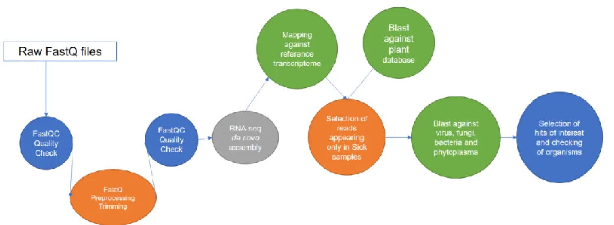
(10) pathogen, and the pipeline followed in this project would be very useful to analyze the data, especially in the case of a non-published genome of the infected plant. 1.2 Objectives of the project The main objectives and sub-objectives of this project are: 1. Create a pipeline to analyze sequences of healthy and diseased leek plants from RNA-seq results. It is necessary to develop an accurate and practical pipeline which includes steps of data preprocessing and comparative analysis between infected and healthy plants. 1.1. Prepare and install Linux environment in the computer. 1.2. Acquire skills in data manipulation. 1.3. Understand and apply the necessary steps to analyze the NGS data. 1.4. Acquire skills to solve the problems that may arise. 2. Identify the microorganisms found in the samples with an effective pipeline. 2.1. Identify the microorganisms found in the diseased samples but not in the healthy ones. The associated microbiota of healthy and infected leeks will be decisive to identify the microorganism or microorganisms that are causing the disease, which would appear exclusively in the infected plants and not in the healthy plants. 3. Associate microorganisms observed only in infected plants with the cause of the symptomatology observed in infected plants. Microorganisms appearing exclusively in with the infected plants could be not responsible for the symptoms, so it is important to investigate if they are plant pathogens related to leeks or other plants. 1.3 Approach and methods There are two plausible approaches for trying to identify the pathogen using the RNA-seq data. The first approach is to select all the sequences that do not map against a de novo assembly transcriptome built with all the Control sample reads. The second approach is to assemble a transcriptome that includes all the reads from all the samples (Sick1, Sick2, Sick3, Sick4 and Control). This assembly is set as the reference transcriptome (for this project) and to which all samples are later mapped. All those reference transcripts with mapped reads from the sick samples but not from the control are potential transcripts of interest, since they could belong to the microorganisms causing the disease. Both approaches need common preliminary steps that include: - Quality control analysis of the raw reads to identify possible sequence of adapters remaining after the trimming of the NGS service.. 3.

(11) - Trimming of adapters that have previously been selected and trimming of lowquality sequences (especially at the ends of the reads). - Pairing sequences to convert single reads in pair ends. Both strategies are considered an adaptation of a typical RNA-seq pipeline. Nevertheless, they include an assembly de novo of the transcriptome due to the lack of the leek genome in databases. The second strategy is selected in this project, using as reference a de novo assembly transcriptome of all the reads. In this approach, after the assembly, reads of the Control and Sick samples are mapped against the assembly and all the control reads mapping against the transcriptome are discarded. In this approach, it is created a table of counts that includes the transcripts of the reference transcriptome and the number of times that they have appeared in the samples. Transcripts of interest will be those which appear exclusively in the Sick pools. This step has two main advantages, it reduces the number of possible reads to analyze and it generates the table of counts as a practical and intuitive tool to work with the results. Later on, we can use this table to easily filter by different parameters and select transcripts of interest. Finally, we will blast the selected transcripts against NCBI database of plants to discard plant proteins. After this filtering, we will blast the resulting transcripts against NCBI database of several plant pathogens to obtain a list of possible candidate microorganisms causing the disease. The proposed pipeline for the analysis is detailed in Figure 3.. Figure 3. Workflow followed for the final project master.. 4.

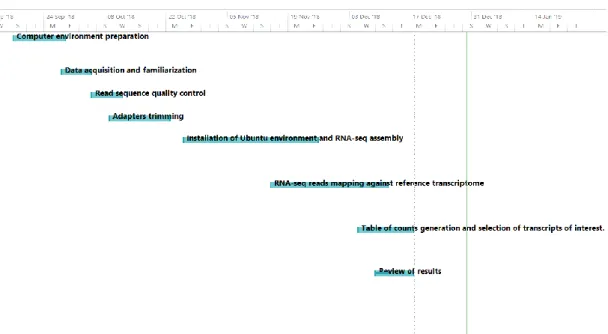
(12) 1.4 Planning. Figure 4. Gantt diagram showing the planning followed for the final project master. The tasks defined for this project and planned according to the Figure 4 diagram are: 1. Computing environment preparation. Installation of a full Ubuntu operative system in an empty computer. 2. Data acquisition and familiarization Acquisition of the data by transferring it to an external hard drive (2 TB capacity). 3. Read sequence quality control Quality control check of raw data with the software FastQC that also provides information about the presence or absence of adapters (Leggett et al., 2013). 4. Adapters trimming Trimming of the adapters with Trimmomatic. It is an efficient preprocessing tool that can handle paired-end data and also provide the paired ends that survived to the preprocessing (Bolger et al., 2014). 5. Assembly de novo of a reference transcriptome Assembly de novo of a reference transcriptome since there is not a published leek genome or transcriptome. This assembly was performed by Trinity, a. 5.

(13) powerful tool which can handle single and paired-end data and perform assemblies in a very effectively (Haas et al., 2013). 6. RNA-seq reads mapping against reference transcriptome The reference transcriptome was established for this project, Control, Sick1, Sick2, Sick3 and Sick4 reads were mapped against it. This alignment was done with Bowtie2, a very fast and memory efficient tool that can find not only short alignments, but also long and gapped ones (Langmead and Salzberg, 2012). 7. Table of counts generation and selection of transcripts of interest. We obtained .bam (binary alignment map) files from the mapping. These files were converted to table of counts by using some of the functions included in the samtools package (Li et al., 2009). These tables show the transcripts present in each one of the samples. In this project, only transcripts exclusively present in the diseased leek samples were selected to continue with the analysis. These transcripts were blasted against the NCBI database to obtain a list of the possible candidate pathogens. The sequences of plants were removed from this list. The transcripts that showed a low percentage of identity with any organism were also removed from the list. 8. Review of the results and validation Finally, the selected transcripts were studied to determine if they belong to microorganisms previously associated with pathogens. The main resource for this step were scientific articles which could mention the selected microorganisms as responsible of diseases related to leek or other related species. 1.5 Short summary of obtained products The products obtained in the steps of the followed pipeline are: 1. FastQC Quality Check. FastQC create reports in .html format that includes basic statistics and graphics related to the quality of the sequence, adapters identification. 2. Trimming of adapters. After trimming, we obtained the trimmed pairedend reads. 3. FastQC Quality Check after trimming. New quality check to obtain good quality sequences for the rest of the analysis. 4. Assembly de novo. The trimmed sequences were used to create an assembly de novo of all the samples. The resulted assembly consisted of a FASTA file that included a list of the assembled transcripts with new IDs.. 6.

(14) 5. Mapping against reference transcriptome. A mapping of each of the trimmed paired-end reads was performed and .sam (Sequence alignment map) files were obtained. Files .sam were converted into .bam (binary alignment map) files. Finally, these files were translated in a table of counts (a R data frame with one column containing transcripts ID and the rest, specifying the number of mapped reads for the pool). 6. Blast against plant database. The transcripts of interest were uploaded in the NCBI blast database to generate a list of hits and their characteristics. The list of hits from the blastx search was obtained in a .csv file with columns containing alignment features. 7. Filtering of plant proteins. The .csv file was converted into a new table of counts in R. This table was used to filter hits that aligned with plant sequences with high percentage identity at aminoacidic level. 8. Blast against virus, fungi, viroids, bacteria and phytoplasmas databases. After filtering plant sequences, a new blast search was done to identify all the microorganisms. Hits resulted from the blastx search were organized in text file. 9. Selection of transcripts of interest. The text file, containing the hits of blastx in R, was uploaded to filter the results. The hits showing a higher percentage of identity were filtered and saved in a new text file named as id_selected.txt file. This file contained a list of possible identifiers of pathogens that cause the disease. This file was uploaded in the Batch Entrez application of NCBI. This tool takes as input a list of NCBI identifiers and returns a list of proteins and microorganisms associated to the sequences. Finally, the resulting list of protein names and organisms were downloaded in a summary file in .txt format. 1.6 Short description of chapters of the memory This memory aims to explain the pipeline followed for the analysis of the RNAseq pools. It is very important to explain each of the steps in the workflow, including the software or commands applied, its functions, the content of the input and the output and the alternative ways to analyze the data. Therefore, there is one chapter for each of the main steps of the analysis. The titles of these chapters are: 2.1. Computer environment preparation. 2.2. Quality control analysis before and after trimming using FastQC. 2.3. Trimming of adapters with Trimmomatic. 2.4. Assembly de novo of reference transcriptome using Trinity. 2.5. Mapping against reference transcriptome with Bowtie2. 2.6. Selection of transcripts of interests. 2.7. Table of counts generation and selection of transcripts of interest. 2.8. Results. 7.

(15) 2. Chapters 2.1. Computing environment preparation The first computing environment preparation step was to install an Ubuntu terminal in a Windows 10’s Bash Shell to install the bioinformatic software and run commands from this shell (Morais et al., 2018). It was of the most recent advances to keep working with all the tools of Windows and at the same time make profit of the bioinformatic software developed for Ubuntu systems. Nevertheless, after working some time with it, it was found out that this environment was not prepared to install some of the software and run some of the commands. Some reiterative errors appeared while installing most of the packages, so it was decided to use a complete Ubuntu environment. This would assure to have less problems with the installation of bioinformatic packages and less errors in their performance. For the installation of the Ubuntu system, the .iso image of the last version of Ubuntu (Ubuntu 18.04.1) was saved in a bootable USB flash drive. Then, it was booted it in an HP Pavilion computer provided with Intel® Core™ i5-2410M CPU @ 2.30GHz × 4. The former operative system (Windows 7) was fully removed in order to have full capacity of the computer. Once Ubuntu was working correctly, some essential packages to perform all the analysis were installed. -. Conda. Conda (https:// conda.io) is a powerful manager package that includes a wide list of the main bioinformatic packages applied nowadays (Grüning et al., 2018). It exists a heterogeneity in the installation methods and in the programing languages that are available for bioinformatic analysis. Its use avoids some of the most common resulting errors that appear when software is downloaded and installed in different operating systems. In other words, Conda provides a normalization in the installation of many bioinformatic tools. -. R and RStudio. R is the free computational environment which includes a wide range of packages for many areas of science. In the case of bioinformatics, R language includes a set of packages that can analyze genomic and transcriptomic data (Eglen, 2009). For example, Bioconductor provides a set of packages that analyze genomic data or, other packages as seqinr, which manages sequence data formats (Bastolla, 2007). 2.2. Data acquisition and familiarization Data was transferred from a server to an external drive (2TB capacity). Data consisted of 10 files. The names of the files were changed to shorter ones and the files were uncompressed to facilitate its handling. Previous and new names of the files and its size are shown in Figure 5. 8.

(16) Previous file names. New file names. File Size (Gigabytes). PC-_22512_ATCACG_read1.fastq.gz PC-_22512_ATCACG_read2.fastq.gz P1_22513_CGATGT_read1.fastq.gz P1_22513_CGATGT_read1.fastq.gz P2_1_sick.fq P2_2_sick.fq P3_1_sick.fq P3_2_sick.fq P4_1_sick.fq P4_22516_GTCCGC_read2_fastq. PC_1.FQ PC_2.FQ P1_1.FQ P1_2.FQ P2_1.FQ P2_2.FQ P3_1.FQ P3_2.FQ P4_1.FQ P4_2.FQ. 1.9 2.0 1.4 1.6 4.2 3.9 7.2 5.6 10.3 11.5. Sample name to use in this project Control₁ Control₂ Sick1_1 Sick1_2 Sick2_1 Sick2_2 Sick3_1 Sick3_2 Sick4_1 Sick4_2. Conditions. Read. Pool control Pool control Pool sick 1 Pool sick1 Pool sick 2 Pool sick 2 Pool sick 3 Pool sick 3 Pool sick 4 Pool sick 4. 1 2 1 2 1 2 1 2 1 2. Figure 5. Table of main characteristics of files and new names assigned. 2.3. FastQC quality control analysis before and after trimming First, quality control analysis of the sequences was performed with FastQC software. FastQC took as input the fastq files and provided an assessment of the overall quality of the sequences. It was necessary to check that the sequencing was correctly done and data was suitable to follow the successive steps. FastQC produce a fastqc_report.html that shows a series of images and graphics representing the sequencing quality in an easy-to-read format. In the next lines are explained the most important sections of the report and are shown the results of the quality control analysis for the samples Control, Sick1, Sick2, Sick3 and Sick4. Basic statistics Basic statistics show basic information about the RNA-seq raw data as number of sequences and sequence length. The basic statistics results (Figure 6) showed that all the libraries have good quality. BEFORE TRIMMING. AFTER TRIMMING. 1. Total sequences 22286519. Sequence length 151. Total sequences 18578855. 2. 22286519. 151. 18578855. Pool sick 1. 1. 16283248. 151. 12647070. Pool sick1. 2. 16283248. 151. 12647070. Sick2_1. Pool sick 2. 1. 27274984. 40-151. 12068165. Sick2_2. Pool sick 2. 2. 12075692. 40-151. 12068165. P3_1.FQ. Sick3_1. Pool sick 3. 1. 21876090. 40-151. 17383236. P3_2.FQ. Sick3_2. Pool sick 3. 2. 17395508. 40-151. 17383236. P4_1.FQ. Sick4_1. Pool sick 4. 1. 31045565. 40-151. 10334054. P4_2.FQ. Sick4_2. Pool sick 4. 2. 32855303. 151. 10334054. ORIGINAL NAME PC_1.FQ. Sample name Control_1. Conditions. Read. Pool control. PC_2.FQ. Control_2. Pool control. P1_1.FQ. Sick1_1. P1_2.FQ. Sick1_2. P2_1.FQ P2_2.FQ. Sequence length 36-151. Figure 6. Summary table of main characteristics of FastQC files. The file types were conventional base calls and the encoding Sanger/Illumina 1.9.. 9.

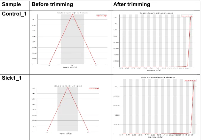
(17) N content per sequences and percentage of sequences flagged as poor quality The N content per sequence and the percentage of sequences flagged as poor quality were 0%. Sequence length distribution It plots a graph showing the distribution of fragment sizes. In this case, graphics showed that was mainly concentrated at the maximum length (151 pb) for all the samples. We show the sequence length distribution graphs for samples Control_1 and Sick1_1 in Figure 7. Rest of the graphs showed are shown in the annexes (Figure 18). Sample. Before trimming. After trimming. Control_1. Sick1_1. Figure 7. Sequence length distribution graphics for samples Control_1 and Sick1_1. Quality scores graphics The quality control analysis also provided quality scores graphics. These graphics show the nucleotide quality in each sequencing cycle. Most of the nucleotide position appeared in the green zone indicated a good quality of the sequences before trimming. The quality scores graphics of samples Control and. 10.

(18) Sick1 are shown in Figure 8. All the quality scores graphics are represented in Figure 19. Sample. Before trimming. After trimming. Control_1. Sick1_1. Figure 8. Quality score graphics of samples Control and Sick1 before and after trimming. Per Tile Sequence quality graphics Per Tile Sequence quality graphic indicated the deviation from the average quality for each tile. Cold colors showed the positions where the quality is at or above the average for that base in the run. In the case of the samples to analyze, all of them presented a predominantly dark blue and a low presence of hot colors in the graphic. Per Tile Sequence quality graphics of samples Control_1 and Sick1_1 are shown in Figure 9. Graphs of all the samples are shown in Figure 20 of the annexes section.. 11.

(19) Sample. Before trimming. After trimming. Control_1. Sick1_1. Figure 9. Per tile sequence quality graphics of samples Control_1 and Sick1_1 before and after trimming. Per sequence quality scores graphics These graphics show if a subset of the sequences has universally low-quality values. We show graphics resulted before and after trimming the samples Control_1 and Sick1_1. As it can be seen in Figure 10, graphics show that Q40 has more read number than other quality scores. Graphics of all the samples are shown in Figure 21 in the Annexes section.. 12.

(20) Samples. Before trimming. After trimming. Control_1. Sick1_1. Figure 10. Per sequence quality scores graphics samples Control_1 and Sick1_1. Adapter content Adapter content graphics show the percentage and type of adapters present in the samples. Graphs of samples Control_1 and Sick1_1 are shown in Figure 11. Adapter content was under 5% in all the cases indicating that there was a low percentage of contamination in the samples (Figure 12). The universal adapter of Illumina TruSeq was the only adapter in the samples. Graphics of all the samples are shown in Figure 22 in the annexes section. Sample. Before trimming. After trimming. Control_1. 13.

(21) Sick1_1. Figure 11. Adapter content of samples Control_1 and Sick1_1. Other graphics The rest of the graphics included in the report showed almost the same results for untrimmed and trimmed sequences. -. Per base sequence content graphic. It plots out the proportion of each base position. In the case of our samples, the number tends to stabilize from 15-18 pb position.. -. Per sequence GC content. It plots the GC content across the whole length of each sequence. It plots two lines, a blue line showing the theoretical distribution and a red line showing the GC content. This graphic must show a Gaussian distribution.. -. Per base N content. It plots out the percentage of base calls at each position for which an N was called. All sample present 0% of N content.. -. Sequence duplication levels. The degree of duplication for every sequence in a library is count and a plot is created showing the relative number of sequences that have different degrees of duplication. This graph does not change when the trimming is applied.. -. K-mer content. This parameter indicates the number of each 7-mer at each position in the library and applies a binomial test to search for significant deviations from an even coverage at all positions. Any Kmers showing positional biased enrichment are reported. The top 6 most biased Kmer are plotted to show their distribution.. Graphics mentioned above and resulted in the report of Control_1 sample are included in Figure 12. In case of any of these figures wanted to be consulted, a zip folder containing the complete reports has been added to this delivery (Supplementary data 1). Its content is explained in the Supplementary Data section.. 14.

(22) Type of Before trimming graphics. After trimming. Per base sequence content. Per sequence GC content. Per base N content. Sequence duplication levels. K-mer content. Not included in the trimming files. Figure 12. Other graphs included in the report of Control_1.. 15.

(23) 2.4. Trimming of adapters with Trimmomatic NGS services might make a preprocessing of the raw reads in order to trim the adapters included for the sequencing process. Nevertheless, it is always necessary to check if some adapters remain because residual adapters can generate suboptimal downstream analyses. There are multiple bioinformatic tools that trim adapters such as cutadapt (Martin, 2011), AdapterRemoval v2 (Martin, 2011), Skewer (Jiang et al., 2014) or Trimmomatic (Bolger et al., 2014) among others. Trimmomatic was selected because it includes a very sensitive and specified step of technical sequences removal of paired-end data. This tool finds matches of partial or complete technical sequences as adapters, polymerase chain reaction (PCR) primers and other fragments in paired-end reads. This mode of working is called palindrome mode and include some steps. First, there is a search of overlaps between the adapters and the opposite reads. In case of finding a complete overlapping, both reads are discarded (Figure 13.A). Then, the search continues “backwards” to find new reads with longer overlapping between them (Figure 13.B). These longer sequences get trimmed too. Trimmomatic also can find other cases where only a small fragment of the adapter is the one overlapping and it trimmed then (Figure 13.C). Finally, the analysis finishes when no more adapters are found in the overlapping regions (Figure 13.D) (Bolger et al., 2014).. Figure 13. Steps of palindrome mode trimming of Trimmomatic. First, overlaps between adapters and reads are found (A), then, a test is run to identify larger 16.

(24) overlaps (B). Also, partial adapters are trimmed (C) and the process finishes when the overlap does not show read-through into the adapters (Bolger et al., 2014). Before using Trimmomatic, an analysis of the presence of some Illumina Universal adapters in raw reads was performed by counting the number of times that they appear. This analysis was performed by searching with grep command and counting the number of lines where the adapter appeared. Trimmomatic can be applied in different ways (Galaxy online software or Linux terminal). In this project was applied it using Linux commands in order to improve bioinformatic skills in this system. First, Trimmomatic was installed using conda package. Then, it was run using as input reads 1 and 2 of the five samples. The parameters of the commands are explained here: -. -. 4 output files referring to the paired and unpaired reads. ILLUMINA CLIP: type of adapter to be removed. In this case, as Illumina universal adapter appeared in 5% of the reads, Truseq was used as the main adapter to trim because appeared at least 80000 in the raw.fastq file. Numbers appearing after the adapter sequence are: o Seed mismatches: selects the maximum count o Palindrome clip threshold: selects the accuracy of the match between the adapter ligated reads o Simple clip threshold: selects the accuracy of the match between the adapter and reads LEADING: indicates the minimum quality that is required to keep a base in the leading part of the sequence. TRAILING: indicates the minimum quality that is required to keep a base in the trailing part of the sequence. SLIDING WINDOW: indicates the number of bases used to average across. MINLEN: specifies the minimum length for the reads that are going to be kept.. After the trimming, four files for each sample were obtained: forward and reverse paired and forward and reverse unpaired. The trimmed reads were reanalyzed with FastQC to determine the differences between quality scores before and after trimming. 2.5. Assembly de novo of reference transcriptome using Trinity In order to reconstruct and identify the full set of transcripts present in our samples, a de novo transcriptome assembly was performed. For this purpose, the trimmed reads of our 5 RNA-seq samples was used: - Control reads - Sick1 reads - Sick2 reads - Sick3 reads. 17.

(25) - Sick4 reads The assembly of all this samples, will be the “reference transcriptome”, and it will contain the full set of RNAs that were sequenced, including the RNAs of the leek plant, as well as the ones from the microorganisms associated with the plant. For the purpose of performing the assembly, forward and reverse files were concatenated using the next commands in Linux terminal. The main software to do assembly de novo from NGS data is Trinity (Haas et al., 2013). This tool can make the reconstruction of the transcriptome in a simple interface and without need of tuning almost any parameters. Its pipeline includes three consecutive modules: Inchworm, Chrysalis and Butterfly (Figure 14). The first module, Inchworm, assembles the reads into contigs in several steps. It builds a k-mer dictionary taking all sequence reads and select the most frequent ones (removing those that may cause errors in the analysis) and extends reads to both sides to obtain longer k-mers. The second module, Chrysalis, clusters the resulted contigs to process them to a de Bruijn graph component. De Bruijn graphics is of the most used formula to find overlaps between reads. Every cluster shows the transcriptome variety for a given gene or set of gen. The last step is to partition all the reads among the disjoint graphs generated before. The third module, Butterfly, finishes the analysis by processing all the graphs in parallel and to create a list of full-length transcripts.. Figure 14. Scheme of basic modules included in Trinity and its use (Haas et al., 2013). The modules Inchworm and Chrysalis require high memory, at least 1 G of RAM per 1M pairs of Illumina reads. In case of assemblies of big files, as in this. 18.

(26) project, it is not possible to run the analysis in a regular computer, then, access to a supercomputer was required. First, Galaxy, was used to try to solve the problems of high memory requirement. It consists of an interactive system with a wide variety of bioinformatic applications. One of its main advantages is that provides substantial CPU and disk space (250 G) for every user (Giardine, 2005) in addition of including many bioinformatics applications. The fastq files (Forward.fq and Reverse.fq) previously obtained concatenating all the reads of the same orientation from the 5 RNA-seq samples were uploaded. Then, Trinity was launched with the default options: Strand-specific Library Type: Group pairs distance: Path reinforcement distance:. Not set 500 75. Nevertheless, when the analysis took more than three days, the server reported an error of exceeded time. After that, another more powerful supercomputer service was used. The supercomputer services provided by CESGA (Fundación Pública Galega Centro Tecnolóxico de Supercomputación de Galicia) was used. Their supercomputer, called Finis Terrae, consists of computation cluster based on Intel Haswell processors. It is composed by 320 compute nodes based on Intel Haswell processor and interconnected with Infiniband network. There are different type of nodes depending of the job requirements. To use the cluster, the user should submit a batch script specifying the type of node, number of cores, memory requirements and time of the process. Once obtained the access to CESGA, Fillezilla, a system specialized in transferring files from different servers, was installed, to save the files in the server to perform the analysis. The total size of the files was almost 50 GB, then, the transfer took two days to be completed. Then, a .sh executable file containing the Trinity commands was created with the next information. #!/bin/bash #SBATCH -t 1-00:00:00 srun Trinity --seqType fq --left Forward_s.fq --right Reverse_s.fq --max_memory 2000G --CPU 10 --no_version_check Then, the job was submitted by running the next commands in the server: sbatch. --partition fatnode -n 1 -c 10 --mem 2000G trinity.sh. --partition: indicates the node type, in this case fatnode. It is a node with 128 cores and 4TB of memory, the only one that could afford the memory requirements of the Trinity assembly. -n: indicates the number of nodes -c: indicates the number of cores 19.

(27) --mem: indicates the maximum memory for each core. Trinity.sh: the executable file where the commands are set. The server reported some memory errors. The analysis required higher amount of memory and several cores, and a wide variety of jobs that required different number of cores and gigabytes of memory were necessary to submit. Trinity required at least three days to complete the assembly, then, only an aleatory sample of 10 % of the sequences of each .fastq file to as a subsample of all the samples was used to continue with the development of the bioinformatics pipeline. The subsampling was run by using the seqtk package, a toolkit to process sequences in Fasta/Fastq formats. Then, the resulting sequences were concatenated in two files Forward_20.fq and Reverse_20.fq Trinity was run using the generated files. A new executable file called Trinity_10.sh was run, where the names of the files were changed, and a new option was selected in order to avoid memory problems with the Butterfly module. #!/bin/bash #SBATCH -t 1-00:00:00 srun Trinity --seqType fq --left Forward_10.fq --right Reverse_20.fq -max_memory 2000G --CPU 10 --no_version_check –bflyCalculateCPU Then, the executable terminal was run in the terminal of the supercomputer. sbatch --partition fatnode -n 1 -c 10 --mem 2000G trinity_10.sh The result of this assembly was a file named as Trinity.fasta that was used as a reference transcriptome. The transcriptome was visualized with Bandage, an interactive visualizer of de novo assemblies (Wick et al., 2015). 2.6. Mapping against the new created transcriptome with Bowtie2 Once the transcriptome was ready, trimmed reads were mapped against it. The chosen software for this mapping was Bowtie2, an aligner that is able to make alignments very fast and memory-efficient while the sensitivity and the accuracy of the results are assured (Langmead and Salzberg, 2012). Bowtie2 does the alignment in four steps. First, “seed” substrings and their reverse complement reads are extracted in full-text minute index. Second, they are aligned to the reference taking ungapped and paired-end regions. The third steps consisted of calculating the seed alignment and its position in the reference. Finally, these seeds are extended into full alignments. Bowtie2 needed two basic commands to run the analysis with the reference transcriptome and the samples. First, it was necessary to create the bowtie index containing the ids of the transcripts of the reference transcriptome. This reference 20.

(28) was composed by several files of type .bt2. Once the index was established, Bowtie2 was run against the four samples. The ideal situation is to have this reference set in the same folder of the fastq files. The resulted .sam files were converted to .bam files with the samtools package, a bioinformatic package which includes universal tools to process read alignments (Li et al., 2009). Binary files are necessary to run the successive steps of the analysis. Samtools was installed using the bioconda installation commands. Later on, .sam files were converted to .bam files and sorted by position. Then, the indexes were created to assure a fast random access. Finally, the ids statistics of the files were exported to .txt files The resulted .txt files contained tables with the information of the number of reads mapping in each reference transcript of each sample. Using these “tables of counts” those transcripts exclusively present in the diseased leek samples were selected. 2.7. Table of counts generation and selection of transcripts of interest 2.7.1. Selection of transcripts of interest The basic packages of R were used to analyze the table of counts and select reads. Also, the R-package “seqinr” was used in order to read and create .fasta files (Charif D. and Lobry J.R., 2007). Raw table of counts contained five columns: - Reference sequence name - Sequence length - Number of mapped reads - Number of unmapped reads The columns of interest were the reference sequence name and the number of mapped reads, that were the ones more interesting in this project. The selection of reads and identification of microorganisms were done applying in R the commands explained in the annex. First, reads with more than 1 mapped read in each of the infected samples (Sick1, Sick2, Sick3 and Sick4) and 0 mapped reads times in the Control were extracted. Then, the selected reads were added in a new .fasta file called Selected_sequences.fasta. 2.7.2. Creation of protein local databases The nucleotide sequences of this file were mapped against Refseq protein local databases of virus, viroids, phytoplasmas, fungi and bacteria. First, it was necessary to install the software blast by Conda. Later on, the databases were 21.

(29) downloaded from the NCBI server by selecting all the RefSeq proteins that belong to virus, viroids, phytoplasmas, fungi and bacteria. Once the local databases were established, blastx searches were run using a maximum e-value of 1e-3 (following the commands shown in the Annex). This tool translated nucleotide sequences to protein considering all the possible reading frames The NCBI blast results were exported in a .csv file that were upload again in R. From all these reads, only the ones showing a percentage of identity higher than 75 percent and more than 70 pb were selected. This filter was essential to work with a smaller number of results and guarantee an accurate selection of organisms. The selection of organisms that fulfilled these requirements were saved in a .txt file and was submitted in the Batch Entrez section of NCBI (https://www.ncbi.nlm.nih.gov/sites/batchentrez). In this section, the IDs were associated with their correspondent organisms and a summary of the information about them was provided. The summary was transformed to a table, shown in Figure 23. In addition to the list of IDs of possible organisms causing the disease, an ontology study of the plant proteins present in the diseased leeks was run. First, the selected transcripts were blasted against plant databases of proteins. This filter was easily applied by specifying the plant taxon (taxid: 3193) in the NCBI website. The results were downloaded in XML format to be used in the next step. This study was carried out with Blast2Go, a bioinformatic tool specialized in functional analysis of plant genomics (Conesa and Götz, 2008). This tool accepts many types of inputs, including blast result files in .xml format. After submitting the file in the software, hits showing more than 75 % of identity with plants were selected and annotated. The annotation results were visualized with a table. 2.8. Results The RNAseq raw reads provided showed good quality and low presence of adapters, only 5 percent of the sequences in case of the Control and the Sick1 samples. These adapter mainly were TruSeq from Illumina. After performing the trimming, the paired-end files were reanalyzed again with FastQC and obtained graphs shown in Figures 6, 7, 8, 9, 10, 11 and 12. These graphs showed that the number of sequences decreased (Figure 6) and the length distribution also changed because Trimmomatic shortened some of the reads (Figure 7). It was also observed that quality scores and Per Sequence Quality Scores graphics improved after trimming (Figure 8 and 9). Finally, as it was expected, the adapter content decreased to 0 in all the samples (Figure 11). These results indicated that the trimming resulted satisfactory.. 22.

(30) Taking only the tenth part of the reads of each file, the assembly run successfully, and it could be used to build a correct transcriptome. The assembly de novo was visualized with Bandage. We visualized the assembly with Bandage graphics in order to check how was the resulted assembly. These graphics show the assembled contigs and the connections between them. So, in case of full genomes form just one organism, the typical graph has big connected structures as in the Figure 15.. Figure 15. Examples of Bandage visualizations (Wick et al., 2015). (a) Ideal bacteria assembly on the left and poor bacteria assembly on the left. (b) Salmonella assemblies. (c) 16S rRNA region of a bacterial genome assembly The resulting graph that we obtained of the transcriptome assembly (Figure 16) consisted on a big image full of different length lines. Each of the lines represent a contig and connections show relations between them. In Figure 16 it can be seen that the number of contigs of the assembly is high, but the relation between them is generally poor. This graph is different from those shown in Figure 15 because they represent contigs of plants and their microbiota associated proteins. Figure 17 shows the full image of the graph, where contigs cannot be appreciated.. 23.

(31) Figure 16: partial image of the Bandage graphic resulted from the assembly of ten percent of the sequences.. Figure 17. Full image of Bandage graphic of the reference transcriptome assembly. The assembled transcriptome contained 78,034 reads. After mapping the five samples against this reference transcriptome the transcripts only appearing in the diseased pools (>1 read in each sick sample) and not in the Control 1 were selected, obtaining 12,755 reads. As this number was pretty high to run a blastx search in the NCBI web, it was decided to run local blast searches using local databases.. 24.

(32) The results of blastx for those contigs showed that 61325 mapped with microorganism proteins, but most of them showed low percentages of identity. That is why, hits were filtered selecting only those with a percentage of identity higher than 75 and a read length higher than 70. The filtered hits gave a result of 311 different proteins which belong to different organisms. Among them, plant pathogenic microorganisms were selected and are shown in Figure 23. Among all, based in the symptomatology of the infected plants, phytoplasmas could be the most probable microorganisms causing the disease, especially Onion yellows phytoplasma and Aster yellows phytoplasma. Both were previously reported associated with symptoms in species related to leek (Khadhair et al., 2002). Nevertheless, the results indicated the possible presence of other pathogenic species of phytoplasmas, as Candidatus phytoplasma australiense and Candidatus phytoplasma mali (Davis et al., 1997; Seemuller, 2004). Some soil pathogenic fungi could be also present in the samples: Fusarium meridionale, Mortierella elongate, Wongia spp. And Cadophora. Also, organisms that were not related to plants, but to humans appeared in the Sick pools. In fact, Rhinocladiella similis and Exophiala spp. were pathogenic microorganisms (Cai et al., 2013; Zeng et al., 2007). No virus or viroids were found in the Sick pools. In addition to the previous results, transcripts from plants were annotated to check the type of protein present in the diseased plants and not in the healthy ones. The results of the annotation showed that most of the function of the proteins were related to transporter activity.. 3. Conclusions The results of this final master project have shown that the pipeline developed to analyze the data is powerful and simple. It was possible to associate the symptoms observed in the leek plants with some possible plant pathogens. Since only ten percent of the reads were included in the assembly of the reference transcriptome it would be necessary to get the full reads assembly and repeat the analysis in order to get more significant results. This project has been a continuous challenge because of the obstacles that have appeared during its accomplishment. First, a new Linux environment had to be set in a formatted Windows laptop. Also, one of the transferred files was truncated and the Sick4 samples have been fully available for the analysis later. Then, the assembly did not work as expected in the computer nor in Galaxy, and it was necessary to wait until access to CESGA was completed. Finally, the familiarization with the supercomputer and its use has required a great amount of time, and still some reported errors keep appearing. Despite of the challenges, most of the objectives have been achieved. First, the pipeline has been written and apply to the data using different software and tools, so it has the flexibility to be applied with similar data. Secondly, it has been 25.

(33) possible to find a strategy to identify microorganisms present in all the pools, and pathogens present in the diseased pools but not in the healthy ones. The third objective was to find the cause of the disease by the identification of microorganisms present only in the infected plants, but no in the healthy ones. It will be necessary to obtain the complete reference transcriptome to apply the pipeline correctly and compare the results. Nevertheless, it could be difficult to detect it by RNAseq some transcripts of pathogens, specifically viruses, because its abundance is smaller by several orders of magnitude comparing them with eukaryotes ones (Andrusch et al., 2018). The methodology proposed from the beginning of the project has been the most suitable. Also, the planning designed at the beginning of the project was suitable for the consumption of time of the tasks. Nevertheless, planning had changes along the process because of the computer difficulties mentioned before, especially the environment preparation and the wait until the access to CESGA. In general, all the learning from this project is absolutely useful to finish the assembly of the reference transcriptome in the future. In case of interesting results, like the identification of the pathogen causing the disease in leeks or the discovery of new pathogens, it would be interesting to publish the pipeline and the results. Also, new knowledge acquired is essential to conduct new bioinformatic projects and to confront a future PhD.. 4. Glossary Adapters. Short DNA sequences used to join the reads to sequence to the sequencing platform. Assembly de novo: method to create a transcriptome or genome without the aid of a reference transcriptome or genome. EDL (Emergent disease in leeks). Name assigned in this project to the disease that cause in leeks symptoms as root geotropism and deformation, and leaves and bulb discoloration. NGS (Next Generation Sequencing). DNA sequencing technology which has improved and accelerated the sequencing by applying new technologies. RNA-Seq. Tool to study the transcriptome in high and accurate way by applying NGS technologies.. 26.

(34) 5. Bibliography Andrusch, A., Dabrowski, P.W., Klenner, J., Tausch, S.H., Kohl, C., Osman, A.A., Renard, B.Y., and Nitsche, A. (2018). PAIPline: pathogen identification in metagenomic and clinical next generation sequencing samples. Bioinformatics 34, i715–i721. Bolger, A.M., Lohse, M., and Usadel, B. (2014). Trimmomatic: a flexible trimmer for Illumina sequence data. Bioinformatics 30, 2114–2120. Cai, Q., Lv, G.-X., Jiang, Y.-Q., Mei, H., Hu, S.-Q., Xu, H.-B., Wu, X.-F., Shen, Y.-N., and Liu, W.-D. (2013). The First Case of Phaeohyphomycosis Caused by Rhinocladiella basitona in an Immunocompetent Child in China. Mycopathologia 176, 101–105. Chiotta, M.L., Alaniz Zanon, M.S., Palazzini, J.M., Scandiani, M.M., Formento, A.N., Barros, G.G., and Chulze, S.N. (2016). Pathogenicity of Fusarium graminearum and F. meridionale on soybean pod blight and trichothecene accumulation. Plant Pathology 65, 1492–1497. Conesa, A., and Götz, S. (2008). Blast2GO: A Comprehensive Suite for Functional Analysis in Plant Genomics. International Journal of Plant Genomics 2008, 1–12. Charif D., and Lobry J.R. (2007). Seqin{R} 1.0-2: a contributed package to the {R} project for statistical computing devoted to biological sequences retrieval and analysis. In Structural Approaches to Sequence Evolution: Molecules, Networks, Populations, (New York), pp. 207–232. Davis, R.E., Dally, E.L., Gundersen, D.E., Lee, I.-M., and Habili, N. (1997). “Candidatus Phytoplasma australiense,” a New Phytoplasma Taxon Associated with Australian Grapevine Yellows. International Journal of Systematic Bacteriology 47, 262–269. Eglen, S.J. (2009). A Quick Guide to Teaching R Programming to Computational Biology Students. PLoS Computational Biology 5, e1000482. Giardine, B. (2005). Galaxy: A platform for interactive large-scale genome analysis. Genome Research 15, 1451–1455. Grüning, B., Sjödin, A., Chapman, B.A., Rowe, J., Tomkins-Tinch, C.H., Valieris, R., and Köster, J. (2018). Bioconda: sustainable and comprehensive software distribution for the life sciences. Nature Methods 15, 475–476. Haas, B.J., Papanicolaou, A., Yassour, M., Grabherr, M., Blood, P.D., Bowden, J., Couger, M.B., Eccles, D., Li, B., Lieber, M., et al. (2013). De novo transcript sequence reconstruction from RNA-seq using the Trinity platform for reference generation and analysis. Nature Protocols 8, 1494–1512.. 27.

(35) Jiang, H., Lei, R., Ding, S.-W., and Zhu, S. (2014). Skewer: a fast and accurate adapter trimmer for next-generation sequencing paired-end reads. BMC Bioinformatics 15, 182. Jung, H.-Y. (2003). “Candidatus Phytoplasma ziziphi”, a novel phytoplasma taxon associated with jujube witches’-broom disease. INTERNATIONAL JOURNAL OF SYSTEMATIC AND EVOLUTIONARY MICROBIOLOGY 53, 1037–1041. Khadhair, A.-H., Evans, I.R., and Choban, B. (2002). Identification of aster yellows phytoplasma in garlic and green onion by PCR-based methods. Microbiological Research 157, 161–167. Khemmuk, W., Geering, A.D.W., and Shivas, R.G. (2016). Wongia gen. nov. ( Papulosaceae , Sordariomycetes ), a new generic name for two root-infecting fungi from Australia. IMA Fungus 7, 247–252. Langmead, B., and Salzberg, S.L. (2012). Fast gapped-read alignment with Bowtie 2. Nat. Methods 9, 357–359. Leggett, R.M., Ramirez-Gonzalez, R.H., Clavijo, B.J., Waite, D., and Davey, R.P. (2013). Sequencing quality assessment tools to enable data-driven informatics for high throughput genomics. Frontiers in Genetics 4. Li, H., Handsaker, B., Wysoker, A., Fennell, T., Ruan, J., Homer, N., Marth, G., Abecasis, G., Durbin, R., and 1000 Genome Project Data Processing Subgroup (2009). The Sequence Alignment/Map format and SAMtools. Bioinformatics 25, 2078–2079. Martin, M. (2011). Cutadapt removes adapter sequences from high-throughput sequencing reads. EMBnet.Journal 17, 10. Morais, D.K., Roesch, L.F.W., Redmile-Gordon, M., Santos, F.G., Baldrian, P., Andreote, F.D., and Pylro, V.S. (2018). BTW—Bioinformatics Through Windows: an easy-to-install package to analyze marker gene data. PeerJ 6, e5299. Pérez-López, E., Olivier, C.Y., Luna-Rodríguez, M., Rodríguez, Y., Iglesias, L.G., Castro-Luna, A., Adame-García, J., and Dumonceaux, T.J. (2016). Maize bushy stunt phytoplasma affects native corn at high elevations in Southeast Mexico. European Journal of Plant Pathology 145, 963–971. Pornsuriya, C., Ito, S., and Sunpapao, A. (2018). First report of leaf spot on lettuce caused by Curvularia aeria. Journal of General Plant Pathology 84, 296– 299. Quaglino, F., Maghradze, D., Chkhaidze, N., Casati, P., Failla, O., and Bianco, P.A. (2014). First Report of ‘ Candidatus Phytoplasma solani’ and ‘ Ca. P. convolvuli’ Associated with Grapevine Bois Noir and Bindweed Yellows, Respectively, in Georgia. Plant Disease 98, 1151–1151. Rodríguez Pedroso, A.T., Plascencia Jatomea, M., Bautista Baños, S., Cortéz Rocha, M.O., and Ramírez Arrebato, M.Á. (2015). Actividad antifúngica in vitro de quitosanos sobre Bipolaris oryzae, patógeno del arroz. Acta Agronómica 65. 28.

(36) Seemuller, E. (2004). “Candidatus Phytoplasma mali”, “Candidatus Phytoplasma pyri” and “Candidatus Phytoplasma prunorum”, the causal agents of apple proliferation, pear decline and European stone fruit yellows, respectively. INTERNATIONAL JOURNAL OF SYSTEMATIC AND EVOLUTIONARY MICROBIOLOGY 54, 1217–1226. Travadon, R., Lawrence, D.P., Rooney-Latham, S., Gubler, W.D., Wilcox, W.F., Rolshausen, P.E., and Baumgartner, K. (2015). Cadophora species associated with wood-decay of grapevine in North America. Fungal Biology 119, 53–66. Uehling, J., Gryganskyi, A., Hameed, K., Tschaplinski, T., Misztal, P.K., Wu, S., Desirò, A., Vande Pol, N., Du, Z., Zienkiewicz, A., et al. (2017). Comparative genomics of Mortierella elongata and its bacterial endosymbiont Mycoavidus cysteinexigens: Comparative genomics of Mortierella elongata. Environmental Microbiology 19, 2964–2983. Wang, Z., Gerstein, M., and Snyder, M. (2009). RNA-Seq: a revolutionary tool for transcriptomics. Nature Reviews Genetics 10, 57–63. Wick, R.R., Schultz, M.B., Zobel, J., and Holt, K.E. (2015). Bandage: interactive visualization of de novo genome assemblies: Fig. 1. Bioinformatics 31, 3350– 3352. Zeng, J.S., Sutton, D.A., Fothergill, A.W., Rinaldi, M.G., Harrak, M.J., and de Hoog, G.S. (2007). Spectrum of Clinically Relevant Exophiala Species in the United States. Journal of Clinical Microbiology 45, 3713–3720. (2007). Structural approaches to sequence evolution: molecules, networks, populations (Berlin ; New York: Springer).. 6. Annexes 6.1. Commands applied in Ubuntu bash for the installation and running of the programs. ## Installation of bioinformatic programs # Download de installer in https://www.anaconda.com/download/ # Apply the next commands in the bash terminal to begin the # installation bash Anaconda-latest-Linux-x86_64.sh # Follow the prompts in the installer screen # Install FastQC conda install -c bioconda fastqc. 29.

(37) # Install R-base sudo apt-get install r-base # Install RStudio sudo apt-get install gdebi cd ~/Downloads wget https://download1.rstudio.org/rstudio-xenial-1.1.419amd64.deb sudo gdebi rstudio-xenial-1.1.379-amd64.deb. ## Preparation of files # Uncompress all zip files and moved them to a new folder called data. gzip gzip gzip gzip gzip. -dk -dk -dk -dk -dk. PC_1.fq.fz PC_2.fq.fz P2_1.fq.fz P2_2.fq.fz P4_2.fq.fz. | | | | |. mv mv mv mv mv. PC_1.fq PC_2.fq P1_1.fq P1_2.fq P4_2.fq. ~/data ~/data ~/data ~/data ~/data. # Do the fastq report for each of the files: fastqc fastqc fastqc fastqc fastqc fastqc fastqc fastqc fastqc fastqc. PC_1.fq PC_2.fq P1_1.fq P1_2.fq P2_1.fq P2_2.fq P3_1.fq P3_2.fq P4_1.fq P4_2.fq. ## Search and trimming of adapters # Search and count of number of TruSeq adapters in grep “AGATCGGAAGACCACACGTCTGAAACTCCAGTCA” PC_1.fq | grep “AGATCGGAAGACCACACGTCTGAAACTCCAGTCA” P1_1.fq | grep “AGATCGGAAGACCACACGTCTGAAACTCCAGTCA” P2_1.fq | grep “AGATCGGAAGACCACACGTCTGAAACTCCAGTCA” P3_1.fq | grep “AGATCGGAAGACCACACGTCTGAAACTCCAGTCA” P4_1.fq | conda install -c bioconda trimmomatic # Trimming of adapters with Trimmomatic. 30. the reads wc -l wc -l wc -l wc -l wc -l.

(38) java -jar trimmomatic-0.38.jar PE -phred33 PC_1.fq PC_2.fq output_forward_paired.fq.gz output_forward_unpaired.fq.gz output_reverse_paired.fq.gz output_reverse_unpaired.fq.gz ILLUMINACLIP:TruSeq3-PE.fa:2:30:10 LEADING:3 TRAILING:3 SLIDINGWINDOW:4:15 MINLEN:36 java -jar trimmomatic-0.38.jar PE -phred33 P1_1.fq P1_2.fq output_forward_paired_P1.fq.gz output_forward_unpaired_P1.fq.gz output_reverse_paired_P1.fq.gz output_reverse_unpaired_P1.fq.gz ILLUMINACLIP:TruSeq3-PE.fa:2:30:10 LEADING:3 TRAILING:3 SLIDINGWINDOW:4:15 MINLEN:36 java -jar trimmomatic-0.38.jar PE -phred33 P2_1.fq P2_2.fq output_forward_paired_P2.fq.gz output_forward_unpaired_P2.fq.gz output_reverse_paired_P2.fq.gz output_reverse_unpaired_P2.fq.gz ILLUMINACLIP:TruSeq3-PE.fa:2:30:10 LEADING:3 TRAILING:3 SLIDINGWINDOW:4:15 MINLEN:36 java -jar trimmomatic-0.38.jar PE -phred33 P3_1.fq P3_2.fq output_forward_paired_P3.fq.gz output_forward_unpaired_P3.fq.gz output_reverse_paired_P3.fq.gz output_reverse_unpaired_P3.fq.gz ILLUMINACLIP:TruSeq3-PE.fa:2:30:10 LEADING:3 TRAILING:3 SLIDINGWINDOW:4:15 MINLEN:36 java -jar trimmomatic-0.38.jar PE -phred33 P4_1.fq P4_2.fq output_forward_paired_P4.fq.gz output_forward_unpaired_P4.fq.gz output_reverse_paired.fq.gz output_reverse_unpaired.fq.gz ILLUMINACLIP:TruSeq3-PE.fa:2:30:10 LEADING:3 TRAILING:3 SLIDINGWINDOW:4:15 MINLEN:36. # Concatenate the forward and reverse files. cat output_forward_paired.fq output_forward_paired_P1.fq output_forward_paired_P2.fq output_forward_paired_P3.fq output_forward_paired_P4.fq > Forward.fq cat output_reverse_paired.fq output_reverse_paired_P1.fq output_reverse_paired_P2.fq output_reverse_paired_P3.fq output_reverse_paired_P4.fq > Reverse.fq ## Subsampling and concatenation # A subsample of the 10% of reads was taken in each of the files, using the same seed. seqtk sample -s4 output_forward_paired.fq 0.1 > PC_1_10.fq seqtk sample -s4 output_forward_paired.fq 0.1 > PC_2_10.fq seqtk sample -s4 output_forward_paired_P1.fq 0.1 > P1_1_10.fq 31.

(39) seqtk seqtk seqtk seqtk seqtk seqtk seqtk. sample sample sample sample sample sample sample. -s4 -s4 -s4 -s4 -s4 -s4 -s4. output_forward_paired_P1.fq output_forward_paired_P2.fq output_forward_paired_P2.fq output_forward_paired_P3.fq output_forward_paired_P3.fq output_forward_paired_P4.fq output_forward_paired_P4.fq. 0.1 0.2 0.2 0.2 0.2 0.2 0.2. > > > > > > >. P1_2_10.fq P2_1_10.fq P2_2_10.fq P3_1_10.fq P3_2_10.fq P4_1_10.fq P4_2_10.fq. # Concatenate of subsamples cat PC_1_10.fq Forward_10.fq cat PC_2_10.fq Reverse_10.fq. P1_1_10.fq P2_1_10.fq P3_1_10.fq P4_1_10.fq. >. P1_2_10.fq P2_2_10.fq P3_2_10.fq P4_2_10.fq. >. ## Mapping with Bowtie2 # Build a reference transcriptome with Bowtie2 Bowtie2-build -f reference Trinity.fasta reference_10 # Map against reference transcriptome bowtie2 -x reference_20 PC_bowtie.sam bowtie2 -x reference_20 P1_bowtie.sam bowtie2 -x reference_20 P2_bowtie.sam bowtie2 -x reference_20 P3_bowtie.sam bowtie2 -x reference_20 P4_bowtie.sam. -1 PC_1_20.fq -2 PC_2_20.fq -S -1 P1_1_20.fq -2 P1_2_20.fq -S -1 P2_1_20.fq -2 P2_2_20.fq -S -1 P3_1_20.fq -2 P3_2_20.fq -S -1 P4_1_20.fq -2 P4_2_20.fq -S. ## Samtools package # Samtools installation with conda conda install -c bioconda samtools # Conversion of .sam files to .bam files samtools view -bS PC_bowtie.sam > PC_bowtie.bam samtools view -bS P1_bowtie.sam > P1_bowtie.bam samtools view -bS P2_bowtie.sam > P2_bowtie.bam samtools view -bS P3_bowtie.sam > P3_bowtie.bam samtools view -bS P4_bowtie.sam > P4_bowtie.bam # Sorting of .bam files by position samtools sort PC_bowtie.bam -o PC_bowtie_sorted.bam samtools sort P1_bowtie.bam -o P1_bowtie_sorted.bam 32.

(40) samtools sort P2_bowtie.bam -o P2_bowtie_sorted.bam samtools sort P3_bowtie.bam -o P3_bowtie_sorted.bam samtools sort P4_bowtie.bam -o P4_bowtie_sorted.bam # Creation of .bam indexes samtools index PC_bowtie_sorted.bam samtools index P1_bowtie_sorted.bam samtools index P2_bowtie_sorted.bam samtools index P3_bowtie_sorted.bam samtools index P4_bowtie_sorted.bam # Exportation of ids statistics to .txt files samtools idxstats PC_bowtie_sorted.bam > PC_idxstats.txt samtools idxstats P1_bowtie_sorted.bam > P1_idxstats.txt samtools idxstats P2_bowtie_sorted.bam > P2_idxstats.txt samtools idxstats P3_bowtie_sorted.bam > P3_idxstats.txt samtools idxstats P4_bowtie_sorted.bam > P4_idxstats.txt. ## Table of counts analysis with R # Install packages if if if if if. (!require(utils)) install.packages("utils") (!require(dplyr)) install.packages("dplyr") (!require(seqinr)) install.packages("seqinr") (!require(string)) install.packages("stringr") (!require(rentrez)) install.packages("rentrez"). # Set working directory setwd("C:/Users/anaru/Documents/bowtie2/") getwd(). ## ## ## ## ##. Read files and delete columns v2 and V3 Column 1: shows the transcript identifier Column 2: Reference sequence length COlumn 3: Number of mapped reads Column 4: Number of placed but unmapped reads. columns <- c(1,3) Bowtie2_PC Bowtie2_P1 Bowtie2_P2 Bowtie2_P3 Bowtie2_P4. <-read.table("PC_bowtie.txt")[,columns] <-read.table("P1_bowtie.txt")[,columns] <-read.table("P2_bowtie.txt")[,columns] <-read.table("P3_bowtie.txt")[,columns] <-read.table("P4_bowtie.txt")[,columns]. 33.

(41) ## Bind columns in a table Bt <- NULL Bt <- cbind(Bowtie2_PC, Bowtie2_P1$V3, Bowtie2_P2$V3,Bowtie2_P3$V3, Bowtie2_P4$V3) colnames(Bt) <- c("id", "PC","P1", "P2", "P3","P4") ## Selection of transcripts in diseased samples showing more than 1 hit df_selection <- Bt[Bt$PC == 0 & Bt$P1 > 1 & Bt$P2 > 1 & Bt$P3 > 1 & Bt$P4 >1,] nrow(df_selection) head(df_selection) Selected_ids <- df_selection$id length(Selected_ids) ## Create a fasta file containing ids and the sequences # Read a fasta file as <- read.fasta("assembly_p10.fasta") sel_seq <- as[Selected_ids] write.fasta(sel_seq, Selected_ids, file.out="Selected_sequences.fasta") head (sel_seq). ## Creation of blast databases in bash terminal of Linux # First, protein databases were downloaded from the NCBI server time makeblastdb -in bacteria_plant_prot.fasta -title "bacteria_plant_prot_db" -dbtype prot -out bateria_plant_prot_db -parse_seqids time makeblastdb -in fungi_prot.fasta -title "fungi_prot_db" dbtype prot -out fungi_prot_db -parse_seqids time makeblastdb -in virus_prot.fasta -title "virus_prot_db" dbtype prot -out virus_prot_db -parse_seqids time makeblastdb -in phytoplasma_prot.fasta -title "phytoplasma_prot_db" -dbtype prot -out phytoplasma_prot_db parse_seqids time makeblastdb -in viroids_prot.fasta -title "viroids_prot_db" -dbtype prot -out viroids_prot_db -parse_seqids. 34.

(42) # Then, the blastx searches were run blastx -query Selected_sequences.fasta -db ~/db/bacteria_plant_prot_db -evalue 1e-4 -outfmt "6 qseqid sseqid pident length mismatch gapopen qstart qend sstart send evalue bitscore qlen qcovs" -out ~/bacteria_plant_blastx.out blastx -query Selected_sequences.fasta -db ~/db/fungi_prot_db evalue 1e-4 -outfmt "6 qseqid sseqid pident length mismatch gapopen qstart qend sstart send evalue bitscore qlen qcovs" -out ~/fungi_blastx.out blastx -query Selected_sequences.fasta -db ~/db/phytoplasma_prot_db -evalue 1e-4 -outfmt "6 qseqid sseqid pident length mismatch gapopen qstart qend sstart send evalue bitscore qlen qcovs" -out ~/phytoplasma_blastx.out blastx -query Selected_sequences.fasta -db ~/db/virus_prot_db evalue 1e-4 -outfmt "6 qseqid sseqid pident length mismatch gapopen qstart qend sstart send evalue bitscore qlen qcovs" -out ~/virus_blastx.out blastx -query Selected_sequences.fasta -db ~/db/viroids_prot_db -evalue 1e-4 -outfmt "6 qseqid sseqid pident length mismatch gapopen qstart qend sstart send evalue bitscore qlen qcovs" -out ~/viroids_blastx.out. ## Selection of hits wirh R # Download the table of results and concatenate them virus <- read.table("Virus_blastx.out", header = FALSE) phytoplasma <- read.table("phytoplasm_blastx.out", header = FALSE) fungi <- read.table("fungi_blastx.out", header = FALSE) bacteria <- read.table("bacteria_plant_blastx.out", header = FALSE) results <- rbind(virus, phytoplasma, fungi, bacteria) nrow(results) head(results) # Table of results contain the next columns: # Fields: query id, subject ids, query acc.ver, subject acc.ver, % identity, alignment length, mismatches, gap opens, q. start, q. end, s. start, s. end, evalue, bit_score, query length and query coverage. 35.

(43) colnames(results) <- c("query_id", "subjects_id", "p_identity", "alignment_length", "mismatches", "gap_opens", "q.start", "q.end", "s.start", "s.end", "evalue", "bit_score", "qlen", "qcov") # Hits showing more than a 75% of identity and more than 70 pb were selected selected_org <- results[results$p_identity>75 & results$alignment_length>70,] sel_org_id <- unique(selected_org$subjects_id) n = length(sel_org_id) # Results are saved in a text file where every row corresponds to an id organism. i = 0 k <- NULL for (i in 1:n) {k[i] <- sub(".*\\|(.*)\\|.*", "\\1",sel_org_id[i] , perl=TRUE)} id_organisms <- data.frame(k) write.table(id_organisms, "id_results.txt",row.names=FALSE, col.names = FALSE, quote=FALSE ). 6.2. Graphics obtained in FastQC reports Sample. Before trimming. After trimming. Control_1. Control_2. 36.

(44) Sick1_1. Sick1_2. Sick2_1. Sick2_2. 37.

(45) Sick3_1. Sick3_2. Sick4_1. Sick4_2. Figure 18. Sequence length distribution graphs before and after trimming, for all the samples. Sample. Before trimming. 38. After trimming.

(46) Control_1. Control_2. Sick1_1. Sick1_2. Sick2_1. 39.


(48) Sick4_2. Figure 19. Quality score graphics of all the samples before and after trimming.. Sample. Before trimming. Control_1. Control_2. Sick1_1. 41. After trimming.


(50) Sick3_2. Sick4_1. Sick4_2. Figure 20. Per tile sequence quality graphics of all the samples before and after trimming Samples. Before trimming. 43. After trimming.

(51) Control_1. Control_2. Sick1_1. Sick1_2. Sick2_1. 44.

(52) Sick2_2. Sick3_1. Sick3_2. Sick4_1. Sick4_2. 45.

(53) Figure 21. Per sequence quality scores graphics of all the samples. Sample. Before trimming. After trimming. Control_1. Control_2. Sick1_1. Sick1_2. Sick2_1. 46.

(54) Sick2_2. Sick3_1. Sick3_2. 47.

(55) Sick4_1. Sick4_2. Figure 22. Adapter content of all the samples 6.3. Table of plant pathogenic organisms present in diseased pools Organism information Stunting, yellowing, witches’ broom , phyllody , virescence in garlic and onion (Khadhair et al., 2002) Stunting, yellowing, witches’ broom , phyllody , virescence in garlic and onion. RefSeq ID. Protein. Organism. WP_011412740.1. 30S ribosomal protein S12. Aster yellows witches'-broom phytoplasma. WP_041639868.1. elongation factor G. Aster yellows witches'-broom phytoplasma. ANV81303.1, ANV81304.1, ANV81305.1, ANV81306.1, ANV81307.1, ANV81308.1, ANV81309.1, ANV81310.1, ANV81311.1, ANV81312.1, ANV81313.1. translation elongation factor 1-alpha, partial. Bipolaris oryzae. Rice fungal pathogen (Rodríguez Pedroso et al., 2015). PVH88454.1. putative 14-3-3 family protein ArtA. Cadophora sp. DSE1049. Wood decay of grapevine (Travadon et al., 2015). molecular chaperone DnaK. Candidatus Phytoplasma australiense. Phytoplasma associated with Australian grapevine yellows (Davis et al., 1997). WP_012359027.1. 48.