A particle numerical approach based on the
SPH method for Computational Fluid
Mechanics
I. Colominas, L. Cueto-Felgueroso, G. Mosqueira, F. Navarrina, M.
Casteleiro
Group of Numerical Methods in Engineering (http://caminos.udc.es/gmni)
Civil Engineering School, University of La Coru˜na, SPAIN
Abstract
Meshfree methods have experimented an important improvement in the last decade. Actually, we can say that the emerging meshless technology constitutes the most promising tool to simulate complex problems in the fluid dynamics area. In this paper we present a formulation which combines a Lagrangian description of the fluid movement (following the spirit of Smoothed Particle Hydrodynamics and Vortex Particle Methods) with a Galerkin formulation and Moving Least-Squares approximation. The performance of the methodology proposed is shown through various dynamic simulations, demonstrating the attractive ability of particle meth-ods to handle severe distortions and complex phenomena.
1 Introduction
The ability of the Smoothed Particle Hydrodynamics method to handle severe distortions allows this technique to be succesfully applied to simulate fluid flows in CFD applications. Early SPH formulations included both a new approximation scheme and certain characteristic discrete equations (the so-called SPH equations), which may look quite strange for those researchers with some experience in meth-ods with a higher degree of formalism such as finite elements. The formulation described in this paper follows a different approach, and the discrete equations are obtained using a Galerkin weighted residuals scheme. Although this new state-ment may result somewhat disconcerting for those accustomed to the classical SPH equations, the Galerkin formulation provides a strong framework to develop more consistent and stable algorithms.
2 MLS Shape Functions
One of the meshless interpolation scheme proposed for meshless approximations is the Moving Least Squares (MLS) method [12, 13]. Although different in their formulation, kernel based approximants (Moving Least Squares [14], Reproduc-ing Kernel Particle Method [15]) can be seen as corrected SPH methods, and in practice they are very similar.
Let us consider a functionu(xxxxxxxxxxxxxx)defined in a bounded, or unbounded, domainΩ. The basic idea of the MLS approach is to approximateu(xxxxxxxxxxxxxx), at a given pointxxxxxxxxxxxxxx, through a polynomial least-squares fitting ofu(xxxxxxxxxxxxxx)in a neighbourhood ofxxxxxxxxxxxxxxas:
u(xxxxxxxxxxxxxx)≈ub(xxxxxxxxxxxxxx) =
m
X
i=1
pi(xxxxxxxxxxxxxx)αi(zzzzzzzzzzzzzz)
¯ ¯ ¯
zzzzzzzzzzzzzz=xxxxxxxxxxxxxx=pppppppppppppp
t(xxxxxxxxxxxxxx)αααααααααααααα(zzzzzzzzzzzzzz)¯¯¯
zzzzzzzzzzzzzz=xxxxxxxxxxxxxx (1)
whereppppppppppppppt(xxxxxxxxxxxxxx)is anm-dimensional polynomial basis andαααααααααααααα(zzzzzzzzzzzzzz) ¯ ¯ ¯
zzzzzzzzzzzzzz=xxxxxxxxxxxxxxis a set of param-eters to be determined, such that they minimize the following error functional:
J(αααααααααααααα(zzzzzzzzzzzzzz) ¯ ¯ ¯
zzzzzzzzzzzzzz=xxxxxxxxxxxxxx) =
Z
yyyyyyy yyyyyyy∈Ωxxxxxxxxxxxxxx
W(zzzzzzzzzzzzzz−yyyyyyyyyyyyyy, h) ¯ ¯ ¯
zzzzzzzzzzzzzz=xxxxxxxxxxxxxx
h
u(yyyyyyyyyyyyyy)−ppppppppppppppt(yyyyyyyyyyyyyy)αααααααααααααα(zzzzzzzzzzzzzz)¯¯¯
zzzzzzzzzzzzzz=xxxxxxxxxxxxxx
i2
dΩxxxxxxxxxxxxxx (2)
whereW(zzzzzzzzzzzzzz−yyyyyyyyyyyyyy, h)
¯ ¯ ¯
zzzzzzzzzzzzzz=xxxxxxxxxxxxxxis a symmetric kernel with compact support (denoted by Ωxxxxxxxxxxxxxx) chosen among the kernels used in standard SPH, and the smoothing lengthh
measures the size ofΩxxxxxxxxxxxxxx. The stationary conditions ofJwith respect toααααααααααααααlead to
Z
yyyyyyyyyyyyyy∈Ωxxxxxxxxxxxxxx
pppppppppppppp(yyyyyyyyyyyyyy)W(zzzzzzzzzzzzzz−yyyyyyyyyyyyyy, h) ¯ ¯ ¯
zzzzzzzzzzzzzz=xxxxxxxxxxxxxxu(yyyyyyyyyyyyyy)dΩxxxxxxxxxxxxxx=MMMMMMMMMMMMMM(xxxxxxxxxxxxxx)αααααααααααααα(zzzzzzzzzzzzzz)
¯ ¯ ¯
zzzzzzzzzzzzzz=xxxxxxxxxxxxxx (3)
where the moment matrixMMMMMMMMMMMMMM(xxxxxxxxxxxxxx)is
M M M M MMM M M M MM M M(xxxxxxxxxxxxxx) =
Z
yyyyyyyyyyyyyy∈Ωxxxxxxxxxxxxxx
pppppppppppppp(yyyyyyyyyyyyyy)W(zzzzzzzzzzzzzz−yyyyyyyyyyyyyy, h) ¯ ¯ ¯
zzzzzzzzzzzzzz=xxxxxxxxxxxxxxpppppppppppppp
t(yyyyyyyyyyyyyy)dΩ
x x x x xxx x x x xx x x (4)
In numerical computations, the global domainΩis discretized by a set of n
nodes insideΩxxxxxxxxxxxxxxas quadrature points (nodal integration). Thus, rearranging (3) we can write α α α α ααα α α α αα α α(zzzzzzzzzzzzzz)
¯ ¯ ¯
zzzzzzzzzzzzzz=xxxxxxxxxxxxxx=MMMMMMMMMMMMMM
−1(xxxxxxxxxxxxxx)PPPPPPPPPPPPPP
ΩxxxxWxxxxxxxxxxWWWWWWWWWWWWWV(xxxxxxxxxxxxxx)uuuuuuuuuuuuuuΩxxxxxxxxxxxxxx (5) where the vectoruuuuuuuuuuuuuuΩxxxxxxxxxxxxxxcontains certain nodal parameters of those nodes inΩxxxxxxxxxxxxxx, and
M M M M M M M M M M M M M
M(xxxxxxxxxxxxxx) =PPPPPPPPPPPPPPΩxxWxxxxxxxxxxxxWWWWWWWWWWWWWV(xxxxxxxxxxxxxx)PPPPPPPPPPPPPPtΩxxxxxxxxxxxxxx, being
P P P P P P P P P P P P P PΩxxxxxxxxxxxxxx=
¡ ppppppp
ppppppp(xxxxxxxxxxxxxx1)pppppppppppppp(xxxxxxxxxxxxxx2)· · ·pppppppppppppp(xxxxxxxxxxxxxxnxxxxxxxxxxxxxx)
¢
; WWWWWWWWWWWWWWV(xxxxxxxxxxxxxx) =diag{Wi(xxxxxxxxxxxxxx−xxxxxxxxxxxxxxi)Vi}, i= 1, nxxxxxxxxxxxxxx
(6) The complete details can be found in [15]. In the above equations, nxxxxxxxxxxxxxxdenotes the total number of nodes within the neighbourhood of pointxxxxxxxxxxxxxxandVi andxxxxxxxxxxxxxxi
are, respectively, the tributary volume (used as quadrature weight) and the coordi-nates associated to nodei. Note that the tributary volumes of neighbouring nodes are included in the matrixWWWWWWWWWWWWWWV, obtaining the MLS Reproducing Kernel Particle
Method [15]. Otherwise, we can useWWWWWWWWWWWWWW instead ofWWWWWWWWWWWWWWV being
W W W W WWW W W W WW W
W(xxxxxxxxxxxxxx) =diag{Wi(xxxxxxxxxxxxxx−xxxxxxxxxxxxxxi)}, i= 1, . . . , nxxxxxxxxxxxxxx (7)
which corresponds to the classical MLS approximation (in the nodal integration of the functional (2), the same quadrature weight is associated to all nodes). Intro-ducing (5) in (1) the interpolation structure can be identified as:
b
u(xxxxxxxxxxxxxx) =ppppppppppppppt(xxxxxxxxxxxxxx)M−1(xxxxxxxxxxxxxx)PPPPPPPPPPPPPP
ΩxxxxxxxxxWxxxxxWWWWWWWWWWWWWV(xxxxxxxxxxxxxx)uuuuuuuuuuuuuuΩxxxxxxxxxxxxxx=NNNNNNNNNNNNNNt(xxxxxxxxxxxxxx)uuuuuuuuuuuuuuΩxxxxxxxxxxxxxx (8) And, therefore, the MLS shape functions can be written as:
N NNNNNN
NNNNNNNt(xxxxxxxxxxxxxx) =ppppppppppppppt(xxxxxxxxxxxxxx)M−1(xxxxxxxxxxxxxx)PPPPPPPPPPPPPPΩxxWxxxxxxxxxxxxWWWWWWWWWWWWWV(xxxxxxxxxxxxxx) (9)
It is most frequent to use a scaled and locally defined polinomial basis, instead of the globally definedpppppppppppppp(yyyyyyyyyyyyyy). Thus, if a function is to be evaluated at pointxxxxxxxxxxxxxx, the basis would be of the formpppppppppppppp(yyyyyyyyyyyyyy−hxxxxxxxxxxxxxx). The shape functions are, therefore, of the form
N N N N NNN N N N NN N
Nt(xxxxxxxxxxxxxx) =ppppppppppppppt(00000000000000)M−1(xxxxxxxxxxxxxx)PPPPPPPPPPPPPP
ΩxxxxWxxxxxxxxxxWWWWWWWWWWWWWV(xxxxxxxxxxxxxx) (10)
In the examples presented in this paper, a linear polynomial basis has been used, which provides linear completeness. Respect to the choice of kernel, a wide variety of kernel functions have been proposed in the literature, most of them being spline or exponential functions. We have not found a general criterion for an optimal choice and we use a cubic spline [12, 13].
3 Discrete Equations for Fluid Flow Problems
3.1 Weighted residuals. Test and trial functions.
The meshless discrete equations can be derived using a weighted residuals for-mulation. Thus, the global weak (integral) form of the spatial momentum equation can be written as:
Z
Ω
ρdbvvvvvvvvvvvvvv
dt ·δbvvvvvvvvvvvvvv dΩ =− Z Ω b σ σ σ σ σ σ σ σ σ σ σ σ σ
σ :δbllllllllllllll dΩ + Z
Ω
bbbbbbbbbbbbbb·δbvvvvvvvvvvvvvv dΩ + Z Γ b σ σ σ σσσσ σ σ σσσ σ
σnnnnnnnnnnnnnn·δbvvvvvvvvvvvvvv dΓ (11)
whereΩis the problem domain,Γis its boundary, and certain functionsδbvvvvvvvvvvvvvvandbvvvvvvvvvvvvvv are the approximations to the test and trial functionsδvvvvvvvvvvvvvvandvvvvvvvvvvvvvv.
The spatially discretized equations are obtained after introducing meshless test and trial functions and their gradients in (11) as
δbvvvvvvvvvvvvvv(xxxxxxxxxxxxxx) =
n
X
i=1
δvvvvvvvvvvvvvviNi∗(xxxxxxxxxxxxxx), ∇∇∇∇∇δb∇∇∇∇∇∇∇∇∇ vvvvvvvvvvvvvv(xxxxxxxxxxxxxx) = n
X
i=1
δvvvvvvvvvvvvvvi⊗ ∇xxxNxxxxxxxxxxx i∗(xxxxxxxxxxxxxx) (12)
b vvvvvvv vvvvvvv(xxxxxxxxxxxxxx) =
n
X
j=1
vvvvvvv
vvvvvvvjNj(xxxxxxxxxxxxxx), ∇∇∇∇∇b∇∇∇∇∇∇∇∇∇vvvvvvvvvvvvvv(xxxxxxxxxxxxxx) = n
X
j=1
vvvvvvvvvvvvvvj⊗ ∇xxxxxxxxxxxxxxNj(xxxxxxxxxxxxxx). (13)
Thus, for each node (particle)ithe following identity must hold:
n
X
j=1
Z
Ω
mijdvvvvvvvvvvvvvvj
dt =ffffffffffffff
int
i +ffffffffffffffexti , i= 1, n (14)
where the mass termmij, the internal forces termffffffffffffffinti and the external forces term
fffffff fffffffexti are:
mij =
Z
Ω
ρNi∗(xxxxxxxxxxxxxx)Nj(xxxxxxxxxxxxxx)dΩ (15)
fffffff fffffffint
i =−
Z Ω b σ σ σ σσσσ σ σ σσσ σ
σ∇∇∇∇∇∇∇∇∇∇∇∇∇∇xxNxxxxxxxxxxxx i∗(xxxxxxxxxxxxxx)dΩ, ffffffffffffffexti =
Z
Ω
N∗
i(xxxxxxxxxxxxxx)bbbbbbbbbbbbbb dΩ +
Z
Γ
N∗
i(xxxxxxxxxxxxxx)σσnσσσσσσσσσσσbσnn dnnnnnnnnnnn Γ (16)
The MLS shape functions do not vanish on essential boundaries and, therefore, the boundary integral in (16) can be decomposed as:
Z
Γ
Ni∗(xxxxxxxxxxxxxx)σσnσσσσσσσσσσσbσnn dnnnnnnnnnnn Γ =
Z
Γu
Ni∗(xxxxxxxxxxxxxx)σσσσσσσσσnσσσσbσnnnnnn dnnnnnnn Γu+
Z
Γn
Ni∗(xxxxxxxxxxxxxx)σσσσσσσnσσσσσσσbnnnnnnnnnnnnn dΓn (17)
beingΓuandΓn, respectively, the parts of the boundary where essential and
natu-ral boundary conditions are prescribed andΓ = Γu∪Γn. It is important to remark
Regarding the equation used for mass conservation, its Galerkin weak form is equivalent to a point collocation scheme and, thus, the continuity equation must be enforced at each particlei,
dρi
dt =−ρidiv(vvvvvvvvvvvvvv)i=−ρi
n
X
j=1
vvvvvvv
vvvvvvvj· ∇∇∇∇∇∇∇∇∇∇∇∇∇∇xxNxxxxxxxxxxxx j(xxxxxxxxxxxxxxi) (18)
where expression (13) for∇∇b∇∇∇∇∇∇∇∇∇∇∇∇vvvvvvvvvvvvvvihas been used.
3.2 Numerical Integration
An important issue in meshless methods corresponds to the numerical integration of the weak form, being also the source of well-known inaccuracies and insta-bilities [9, 12, 14]. The main aspects that must be considered when choosing a numerical quadrature for particle methods are: i) the method should provide rea-sonable accuracy, ii) the numerical quadrature should retain the meshless character of the method, and iii) it should be computationally efficient.
Numerical integration –which concerns the nature itself of meshless methods— has received much attention in Galerkin-based meshless formulations (e.g., the EFGM [2]) but it has not been explicitly studied in SPH, probably because nodal integration lies in the basis of its early formulations and the method was consid-ered a collocation method. Nodal integration has been used, at least implicitly, in all SPH formulations [1, 8], and it evidently is the cheapest option that leads to a truly meshless resulting scheme. The nodes are used as quadrature points and the corresponding integration weights are their tributary volumes. However, this inte-gration scheme is also the cause of instabilities in the numerical solution [9, 14].
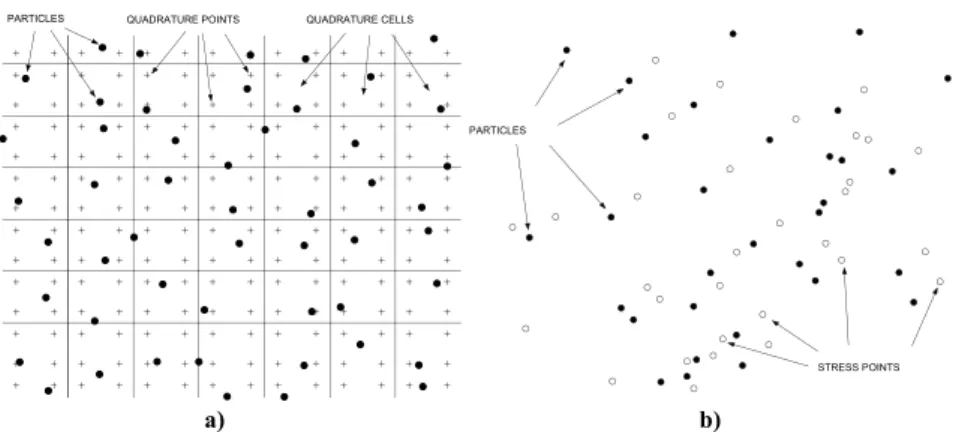
To overcome these problems, some alternatives have been proposed. In the EFG and RKPM methods, it is frequently defined a background integration mesh com-posed by non overlapping cells that cover the whole domain (Figure 1.a), where high order Gauss quadratures are defined [2]. Although these cells do not gener-ally match the integration domains, the spatial framework required by the Galerkin method is recovered (obviously at the cost of the generation of an integration mesh).
In the context of SPH, alternative numerical quadratures have been proposed within the concept of “stress-points”. The idea is essentially to “calculate stresses away from the centroids (the nodes)”, that is, to use a quadrature other than nodal integration in the Galerkin weak form. Then, we must deal with two sets of points: the particles (or nodes) where the MLS-interpolation is defined, and the integration points (the “stress points”), spread among the cloud of particles with no reference to any background mesh (Figure 1.b). Stress points are set up in certain positions and their movement is completely determined by the movement of the particles.
a) b)
Figure 1: Numerical integration: a) Background mesh; b) Particles and stress-points (doble grid)
In references [12, 13] it can be found an extensive revision of these concepts, such as the difference between particle and mesh-based methods regarding numer-ical integration, the nodal integration in the context of the SPH methods, the use of a background integration mesh, the concept of “stress-points” and a new proposal for a more efficient implementation of “stress-points”.
Taking into account these aspects about the numerical integration, we can now write the complete spatially discretized set of equations for a generic integration method. In the following development, we assume a Bubnov-Galerkin scheme where both, the test and trial functions, are chosen from the same space.
For the momentum equation, in practical applications it is not efficient to use the complete mass matrix. Thus, lumped mass matrices are most frequently used. A simple lumping technique corresponds to a row-sum mass matrix; then the discrete counterpart of the lumped mass termMiassociated to particleiis
Mi= ninteX
k=1
ρkNi∗(xxxxxxxxxxxxxxk)Wk (19)
provided that trial functions are, at least, zeroth order complete. If test functions are also zeroth order complete, this lumping is moreover consistent [12]. Taking into account this lumping, the momentum equation results as
Midvvvvvvvvvvvvvvi
dt =ffffffffffffffb
int i +ffffffffffffffb
ext
i , i= 1, n (20)
whereffffffffffffffbinti andbffffffffffffff ext
i are the discrete version of the forces terms (16):
b fffffff fffffffinti =−
ninteX
k=1
b σ σ σ σ σ σσ σ σ σ σ σ σ
σk∇∇∇∇∇∇N∇∇∇∇∇∇∇∇ i(xxxxxxxxxxxxxxk)Wk, ffffffffffffffb ext i =
ninteX
k=1
Ni(xxxxxxxxxxxxxxk)bbbbbbbbbbbbbbkWk+ ninteB
X
k=1
Ni(xxxxxxxxxxxxxxk)σσσσσσσσσσσσσbσknnnWnnnnnnnnnnn kB
whereninteis the total number of quadrature points andninteBis the number of
boundary integration points. Note that appropriate weights,WkandWkB, must be
defined for interior and boundary quadrature points [12].
Now, assuming a compressible newtonian fluid and eulerian kernels [12, 13], the internal forces are related to the Cauchy stress tensor which must be computed at each quadrature point,
b σ σ σσσσσ σ
σσσσσσk=−pkIIIIIIIIIIIIII+ 2µkbdddddddddddddd
0
k (22)
wherepkis the pressure,µkis the viscosity andbdddddddddddddd
0
kis related to the velocity
gradi-ent tensor [12].
Finally, the continuity equation results as
dρi
dt =−ρidiv(vvvvvvvvvvvvvv)i=−ρi
n
X
j=1
vvvvvvv
vvvvvvvj· ∇∇∇N∇∇∇∇∇∇∇∇∇∇∇ j(xxxxxxxxxxxxxxi) (23)
In references [12, 13], it can be found some additional aspects of this numerical approach, such as the performance of the particles movement, the enforcement of the essential boundary conditions, the initialization of the field variables, different alternatives for the discrete equations, the time integration algorithm proposed, and a schematic flowchart and several remarks about the practical implementation of the exposed methodology.
4 Examples and Conclusions
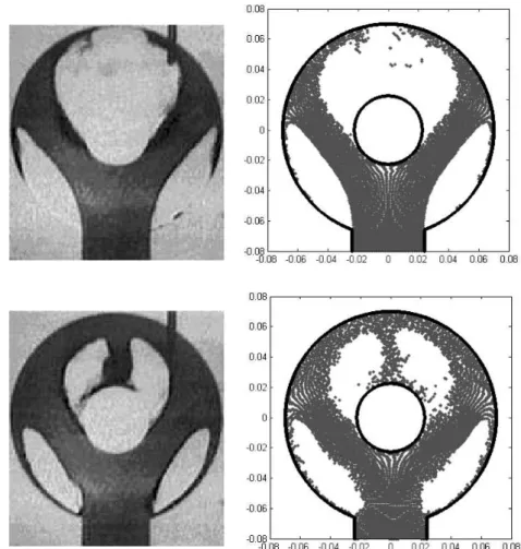
The first example is a simulation corresponding to the filling of a circular mould with core (Figure 2). The velocity of the jet at the gate is18m/sand the viscosity isµ = 0.01kg m−1s−1. The bulk modulus κwas chosen such that the wave celerity is1000m/sand the total number of particles is14314. In Figure 3, two instants of the numerical simulation are shown and compared to the obtained by Schmid and Klein [16].
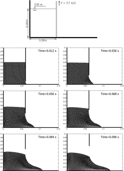
The next example is a fluid-structure interaction problem: the opening of a lock-gate which retains a fluid. The simulation corresponds to the flow of the fluid as the gate rises at a constant speed of0.7m s−1. Figure 4 shows the initial configuration and the simulations at different stages.
70 mm
22,5 mm
45 mm
Figure 2: Mould filling: Dimensions of the mould.
Acknowledgments
This work has been partially supported by the SGPICT of the “Ministerio de Cien-cia y Tecnolog´ıa” of the Spanish Government (Grant DPI# 2001-0556), the “Xunta de Galicia” (Grant # PGDIT01PXI11802PR) and the University of La Coru˜na.
References
[1] J.J. Monaghan. Introduction to SPH. Comp.Phys.Comm. 48:89–96 (1988). [2] T. Belytschko, Y.Y. Lu, L. Gu. Element-Free Galerkin methods.
Int.J.Num.Met.Engrg. 37:229–256 (1994).
[3] L.B. Lucy. A numerical approach to the testing of the fission hypothesis.
Astron.J. 82:1013 (1977).
[4] R.A. Gingold, J.J. Monaghan. SPH: theory and application to non-spherical stars. Month.Not.Roy.Astron.Soc. 181:378 (1977).
[5] L.D. Libersky, A.G. Petschek, T.C. Carney, J.R. Hipp, F.A. Allahdadi. High strain Lagrangian hydrodynamics. J.Comp.Phys. 109:67–75 (1993). [6] P.W. Randles, L.D. Libersky. SPH: Some recent improvements and
applica-tions. Comp.Met.Appl.Mech.Engrg. 139:375–408 (1996).
[7] G.R. Johnson, S.R. Beissel. Normalized Smoothing Functions for SPH impact computations. Int.J.Num.Met.Engrg. 39:2725–2741 (1996). [8] J. Bonet, T-S.L. Lok. Variational and momentum preserving aspects of SPH
formulations. Comp.Met.Appl.Mech.Engrg. 180:97–115 (1999).
[9] J. Bonet, S. Kulasegaram. Correction and stabilization of SPH with appli-cations in metal forming. Int.J.Num.Met.Engrg. 47:1189–1214 (2000). [10] J.K. Chen, J.E. Beraun. A generalized SPH method for nonlinear dynamic
Figure 3: Mould filling:Experimental (left) and numerical (right) results.
[11] G.A. Dilts. MLS Particle Hydrodynamics. Int.J.Num.Met.Engrg. Part I 44: 1115-1155 (1999), Part II 48: 1503 (2000).
[12] L.Cueto-Felgueroso, I.Colominas,G.Mosqueira, F.Navarrina, M.Casteleiro. On the Galerkin formulation of SPH. Int.J.Num.Met.Engrg. [press] (2004). [13] L. Cueto-Felgueroso. A unified analysis of meshless methods: formulation & applications. Technical Report (in Spanish), Univ. de La Coru˜na, (2002). [14] T. Belytschko, Y. Guo, W.K. Liu, S.P. Xiao. A unified stability analysis of
meshless particle methods. Int.J.Num.Met.Engrg. 48:1359–1400 (2000). [15] W.K. Liu, S. Li, T. Belytschko. MLS Reproducing Kernel methods (I).
Comp.Met.Appl.Mech.Engrg. 143:113–154 (1997).
Time=0.012 s Time=0.036 s
Time=0.056 s Time=0.068 s
Time=0.084 s Time=0.096 s