On the Techniques for Measuring Muffling Devices with Flow

G

Guuiimmaarrããeess--PPoorrttuuggaall

paper ID: 98 /p.1

On the Techniques for Measuring Muffling

Devices with Flow

Jorge P. Arenas

, Samir N.Y. Gerges

, Erasmo F. Vergara

, Juan L. Aguayo

a

Universidad Austral de Chile, Institute of Acoustics, Casilla 567, Valdivia, Chile, jparenas@uach.cl

b

Department of MechanicalEngineering, Univ. Federal de Santa Caterina, Florianópolis, Brazil.

ABSTRACT: The characterization of a muffling device used for noise control applications can be given in terms of the attenuation, insertion loss, transmission loss, and the noise reduction. In addition, the four-pole parameters of a muffler can supply important information on the acoustical properties of the device. In certain cases, some of the parameters to measure the performance can be related. It has been commonly accepted that the transmission loss is the most important parameter to characterize the performance of a muffling device. However, there are some discrepancies regarding the most precise method to measure it, in particular, when the effects of a mean flow are needed. In this article some of the techniques used to measure the acoustic performance of muffling devices are described. In particular, the decomposition method, the two-load method, and the two-source method are discussed and its associated errors and limitations are examined. Some numerical and experimental examples on a single expansion chamber are presented. For the numerical results, the finite element method is used to estimate the sound pressure distribution inside each muffling device and, consequently, to predict its properties.

1. INTRODUCTION

There is a growing public awareness of noise nuisance both at work and in the home. Noise appears to have been connected in the public image with pollution in all its forms. It is likely that competitive pressures to produce quieter machinery will parallel this increasing awareness of people about noise. Thus, in the next few years there will probably be increased pressure upon manufacturers and government to reduce the noise from factories, appliances and both private and public transportation.

Exhaust noise of internal combustion engines is known to be the biggest pollutant of the present day urban environment. Fortunately, this noise can be reduced to the level of the noise from other automotive sources by means of a well-designed muffler. Mufflers are conventionally classified as dissipative or reactive, depending on whether the acoustic energy is dissipated into heat or is reflected back by area discontinuities. A simple expansion chamber is, for example, a reactive muffler.

Ideally the noise control knowledge would be most efficiently applied at the design stage before the prototype is built. In principle, such an approach would insure a quieter prototype unit and possibly eliminate the need for expensive noise control measures to be applied in the production stages.

G

Guuiimmaarrããeess--PPoorrttuuggaall

paper ID: 98 /p.2

Therefore, a study of the propagation of waves in tubes or ducts is central to the analysis of a muffler for its acoustic performance (transmission characteristics).

2. CHARACTERIZATION OF THE PERFORMANCE

The performance of an acoustical muffler is measured in terms of one of the following parameters [1]:

2.1. Insertion Loss, IL

Insertion loss is defined as the difference between the sound power levels, Lw, radiated

without any filter (W1) and that with the filter (W2). Mathematically, in dB,

2 1 2

1 10log

W W Lw

Lw

IL= − = . (1)

2.2 Transmission loss, TL

Transmission loss is independent of the source and requires an anechoic termination at the downstream end. It describes the performance of what has been called “the muffler proper”. It is defined as the difference between the power incident on the muffler proper and that transmitted downstream into an anechoic termination.

2.3 Noise reduction, NR

Noise reduction (or level difference) is the difference in sound pressure levels Lp at two

arbitrary selected points in the exhaust pipe and tail pipe. Unlike the transmission loss, the definition of noise reduction makes use of standing wave pressures and do not require an anechoic termination. Therefore, in dB,

1 2 1

2 20log

p p Lp

Lp

NR = − = . (2)

2.4 Attenuation, A

Like noise reduction, Attenuation also refers to the decrease in sound pressure levels between two points. However, attenuation is more commonly used for describing the acoustical properties of heating, ventilating, and air conditioning ducts lined with sound absorbing material. When applied to the acoustic of ducts, Attenuation can be reported in decibels per unit length of duct.

G

Guuiimmaarrããeess--PPoorrttuuggaall

paper ID: 98 /p.3

receiver (the load). However, it requires prior knowledge or measurement of the internal impedance of the source.

Transmission loss does not involve the source impedance and the radiation impedance because it represents the difference between incident acoustic energy and that transmitted into

an anechoic environment. Being made independent of the terminations, TL finds favor with

researchers who are sometimes interested in finding the acoustic transmission behavior of an element or set of elements in isolation of the terminations [1]. In the past, measurement of the incident wave in a standing wave field required use of the impedance tube technology, leading to quite laborious experiments. However, use of the two-microphone method with modern instrumentation allows faster and accurate results.

Noise reduction is the difference in sound pressure levels at two points, one upstream and one

downstream. Like TL it does not require knowledge of source impedance and, like IL, it does

not need anechoic termination. It is therefore the easiest to measure and calculate and has come to be used widely for experimental corroboration of the calculated transmission behavior of a given set of elements (the muffler proper).

Attenuation also depends on source and/or termination impedances as well as the characteristics of the muffler or silencer itself.

3. MEASUREMENT OF THE PERFORMANCE

Measurements are required for supplementing the analysis by providing certain basic data or parameters that cannot be predicted precisely, for verifying the analytical/numerical predictions, and also for evaluating the overall performance of a system configuration so as to check if it satisfies the design requirements [1]. In particular, in the field of exhaust systems, where mean flow introduces quite a few complications, measurements are required for evaluation of radiation impedance or reflection coefficient at the radiation end (tile pipe end). In addition, measurements of flow-acoustic attenuation constant, characteristics of the engine exhaust source, level difference (noise reduction), or transmission loss of one or more acoustic elements are needed in order to verify the transfer matrices, dissipation of acoustic energy emerging from the tail pipe end in the shear layer of the mean-flow jet, and, finally, the insertion loss of the exhaust muffler as required by the designer and user.

Measurement of insertion loss of a muffler is the easiest thing to do since it requires a measurement of sound pressure in the far field without and with the muffler. The output of the microphone is fed through a preamplifier to a spectrum analyzer and from there to a measuring amplifier. Of course, it is important to have a sufficiently anechoic environment so as to ensure that the two positions of the microphone (with and without the muffler) are subjected to almost the same reverberation sound.

G

Guuiimmaarrããeess--PPoorrttuuggaall

paper ID: 98 /p.4

maxima and minima. This is a process very tricky and sometimes inefficient because of certain unsteadiness resulting from the flow-probe interaction and the large number of measurements to do [1]. An alternative to this method is the two-microphone method [2, 3, 4, 5] and certain variants proposed.

3.1 Transfer matrix

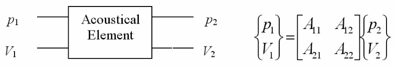
The transfer matrix (also called transmission matrix or four-pole parameter representation) is an approach to model an acoustical element, adopting sound pressure and particle velocity as two state-variables [1]. The transfer matrix equation for an acoustical element is shown in Fig.

1, where p1 and p2 are the sound pressure at the inlet and outlet, respectively, V1 and V2 are the

particle velocities at the inlet and outlet, respectively, and A11, A12, A21, and A22 are the

four-pole parameters of the acoustical element.

Figure 1 – The transfer matrix.

3.2 Two-microphone methods

A two-microphone method, as its name indicates, makes use of two microphones located at fixed positions. The excitation may be a random signal (containing all frequencies of interest) or discrete frequency signal, as used in the probe-tube method. A random noise generator gives the required signal, which is passed through a filter so as to retain only the desired frequency range, and then power amplified before it is fed to an acoustic driver, which creates an acoustic pressure field on the moving medium in the impedance tube (also called

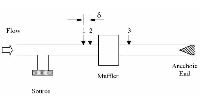
transmission tube). A preamplifier amplifies the signal picked up by each microphone before it is fed to a two-channel Fourier analyzer, which may be controlled by a computer. The measured data are auto-spectral densities of the signals at the two microphone locations and the cross-spectral density between them. Making use of these measured data, the reflection coefficient of the termination is calculated according to the theory. Thus, the real difference between the discrete frequency method of the probe-tube and the two-microphone method is the fact that while the former consists in measuring amplitudes only, the latter measure amplitude as well as the phase difference. The experimental set-up for this method is shown in Fig. 2.

A very useful variant of the two-microphone random-excitation method is the transfer function method presented by Chung and Blaser [3, 4]. The experimental set-up is almost the same, but the reflection coefficient of the termination is calculated from the acoustic transfer

function H12 between the two signals rather than the spectral densities.

G

Guuiimmaarrããeess--PPoorrttuuggaall

paper ID: 98 /p.5

Figure 2 – Experimental set-up for the two-microphone method.

3.3 Decomposition method

The decomposition method was presented by Seybert and Ross [2]. According to the experimental setup shown in Fig. 2, the sound pressure can be decomposed into its incident

and reflected spectra, SAA and SBB, respectively.

For no flow condition, SAA is calculated by the decomposition theory as

δ

δ δ

k

k Q k C S

S

SAA 2

12 12

22 11

sin 4

sin 2 cos

2 +

− +

= , (3)

where S11 and S22 are the autospectra of the total sound pressure at points 1 and 2,

respectively, k is the wave number, δ is the space between the microphones, and C12 and Q12

are the real and imaginary parts of the cross-spectrum between points 1 and 2. In addition, the

root-mean-square amplitude of the sound pressure of the incident sound wave is pi = SAA .

When flow is considered in the decomposition method, a more complicated expression for SAA

is obtained, as a function of the modified wavenumber given as:

V c k

± ω = ±

, (4)

where V is the velocity of the mean flow.

A limitation of the method is that at discrete frequency points for which the microphone spacing is almost equal to an integer multiple of the half-wavelength of sound, an

indetermination occurs. In order to avoid these points up to a frequency fmax, the microphone

spacing δ must be chosen carefully.

Another limitation of the method is that a careful calibration is required for the gain factor as well as the phase factor of the transfer function.

G

Guuiimmaarrããeess--PPoorrttuuggaall

paper ID: 98 /p.6

O i

t i

S S

p p

TL 10log ₂ 10log

2

+

= , (5)

where Si and So are the areas of the muffler input and output, respectively.

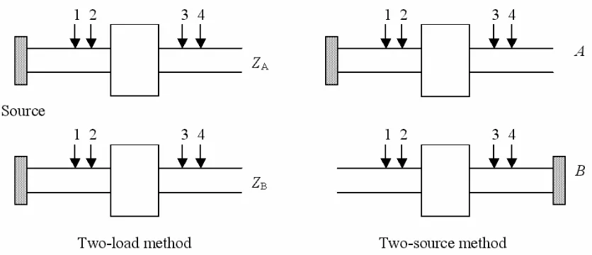
3.4 Two-load method

The two-load method is based on the transfer matrix approach. As it was discussed previously, any muffling element can be modeled by its transfer matrix. In this method, two

different loads (ZA and ZB) must be applied to the output of the system, and then, after

application of the four-pole parameters matrix equation, four unknowns and four equations are obtained [6].

In theory, a load can be any kind of termination (pipe, muffler, anechoic, etc.). Of course, the use of two similar loads will produce unstable results.

3.5 Two-source method

The two-source method was presented by Munjal and Doige [7] and it is also based on the transfer matrix approach. In this method, two sound sources must be placed, firstly at the input of the system and then at the output (Configuration A and B, respectively).

In doing so, four unknowns and four equations are obtained following the application of the four-pole parameters matrix equation (see Fig. 1).

The description of the two-load and two-source methods are presented in Fig. 3. It is very difficult to produce an anechoic termination that allows the passing of a mean flow through the system. Therefore, the decomposition method is less appropriate for measuring the performance of a muffling device when subjected to mean flow.

G

Guuiimmaarrããeess--PPoorrttuuggaall

paper ID: 98 /p.7

4. RESULTS

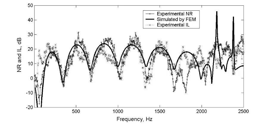
As an example of experimental results obtained for transmission loss, insertion loss and noise reduction, an experiment was performed on a muffler made of a circular simple expansion chamber. Its area ratio (area of the inner chamber to the area of the input pipe) was 16.4. The length of the chamber was 50 cm. The experimental results were compared with the numerical results simulated through a finite element method, and they are presented in Figs. 4 and 5.

Figure 4 – Results obtained for transmission loss for a simple expansion chamber.

G

Guuiimmaarrããeess--PPoorrttuuggaall

paper ID: 98 /p.8

It can be observed a good agreement between the experimental results and the numerical simulation using finite element methods for frequencies up to 1700 Hz. For frequencies above 1700 Hz, the effect of higher modes is relevant, and the assumption of plane wave propagation is no longer valid. In addition, comparing the results presented in Figs. 4 and 5, it is observed that TL is positive while NR and IL can adopt negative values for some frequencies. This means that, at certain frequencies, the noise can be increased.

5. CONCLUSION

This paper has presented the main parameters to describe the performance of a muffling device and the main techniques to measure these parameters. It is clear that the various performance parameters have relative advantages and disadvantages. In terms of the final user, it has been established that the insertion loss is the one that represents the performance of the muffling system, since IL represents the loss in the sound power radiated resulting of the insertion of the muffler between the source and the receiver. In spite of this, and for research purposes, the transmission loss has been widely accepted to evaluate the acoustic transmission behaviour of a muffling element. This is because its theoretical calculation is easier since it does not involve knowledge of the internal impedance of the source and radiation impedance at the end of the system, when energy is transmitted to an anechoic environment. However, the use of finite element approaches allows a quite precise numerical evaluation of the performance of very complicated muffling systems used for noise reduction. Research on this subject is currently under progress for including the effects of mean flow.

ACKNOWLEDGEMENT

This work has been supported by FONDECYT under grants No 1020196 and No 7020196.

REFERENCES

[1] M.L. Munjal, Acoustics of Ducts and Mufflers. John Wiley and Sons, New York, 1987.

[2] A.F. Seybert and D.F. Ross, Experimental Determination of Acoustic Properties using a Two-Microphone Random-Excitation Technique, J. Acoust. Soc. Am. 61(5), 1362-1370, 1977. [3] J.Y. Chung and D.A. Blaser, Transfer Function Method of Measuring In-duct Acoustic

Properties, J. Acoust. Soc. Am. 68(3), 907-921, 1980.

[4] J.Y. Chung and D.A. Blaser, Transfer Function Method for Measuring Acoustic Intensity in A Duct System with Flow, J. Acoust. Soc. Am. 68(6), 1570-1577, 1980.

[5] Z. Tao and A.F. Seybert, A Review of Current Techniques for Measuring Muffler Transmission Loss, SAE Paper 03NVC-38, 2001.

[6] T.Y. Lung and A.G. Doige, A Time-Averaging Transient Testing Method for Acoustic Properties of Piping Systems and Mufflers with flow, J. Acoust. Soc. Am. 73(3), 867-876, 1983. [7] M.L. Munjal and A.G. Doige, Theory of a Two-Source-Location Method for Direct