D2.1 – REPORT ON DYNAMIC DATA
RECONCILIATION OF LARGE-SCALE
PROCESSES
José Luis Pitarch
aCésar de Prada
ba
Research associate (UVA) – Spain
b
Professor (UVA) – Spain
October 2018
Project Details
PROJECT TITLE Improved energy and resource efficiency by better
coordina-tion of produccoordina-tion in the process industries
PROJECT ACRONYM COPRO
GRANT AGREEMENT NO 723575
INSTRUMENT RESEARCH AND INNOVATION ACTION
CALL H2020-SPIRE-02-2016
STARTING DATE OF PROJECT NOVEMBER,1ST2016
PROJECT DURATION 42 MONTHS
PROJECT COORDINATOR (
ORGANIZA-TION) PROF.SEBASTIAN ENGELL (TUDO)
THE COPRO PROJECT
The goal of CoPro is to develop and to demonstrate methods and tools for process monitoring and optimal dynamic planning, scheduling and control of plants, industrial sites and clusters under dy-namic market conditions. CoPro pays special attention to the role of operators and managers in plant-wide control solutions and to the deployment of advanced solutions in industrial sites with a heterogeneous IT environment. As the effort required for the development and maintenance of ac-curate plant models is the bottleneck for the development and long-term operation of advanced control and scheduling solutions, CoPro will develop methods for efficient modelling and for model quality monitoring and model adaption.
The CoPro Consortium
Participant No Participant organisation name Country Organisation 1 (Coordinator) Technische Universität Dortmund (TUDO) DE HES
2 INEOS Köln GmbH (INEOS) DE IND
3 Covestro Deutschland AG (COV) DE IND
4 Procter & Gamble Services Company NV (P&G) BE IND
5 Lenzing Aktiengesellschaft (LENZING) AU IND
6 Frinsa del Noroeste S.A. (Frinsa) ES IND
7 Universidad de Valladolid (UVA) ES HES
8 École Polytechnique Féderale de Lausanne (EPFL) CH HES
9 Ethniko Kentro Erevnas Kai Technologikis Anaptyxis
(CERTH) GR RES
10 IIM-CSIC (CSIC) ES RES
11 LeiKon GmbH (LEIKON) DE SME
12 Process Systems Enterprise LTD (PSE) UK SME
13 Divis Intelligent Solutions GmbH (divis) DE SME
14 Argent & Waugh Ltd. (Sabisu) UK SME
15 ASM Soft S.L (ASM) ES SME
16 ORSOFT GmbH (ORS) DE SME
Document details
DELIVERABLE TYPE REPORT
DELIVERABLE NO 2.1
DELIVERABLE TITLE Report on dynamic data reconciliation of large scale processes
NAME OF LEAD PARTNER FOR THIS DELIVERABLE UNIVERSIDAD DE VALLADOLID
VERSION 2
CONTRACTUAL DELIVERY DATE 31OCTOBER 2018
ACTUAL DELIVERY DATE 31OCTOBER 2018 Dissemination level
PU Public X
CO Confidential, only for members of the consortium (including the Commission)
Abstract
Availability of reliable process information in real time is key in any decision-making procedure. Thus, good industrial decision-support implementations require dealing with gross errors and considera-tion of process transients in order to get a set of measurements which will be coherent with the basic underlying process dynamics. This report presents dynamic data reconciliation methods and tools adapted to the requirements of industrial environments (large-scale systems and noisy/faulty data). Moreover, basic concepts in literature are extended to artificially increase system redundancy as well as to cope with time-varying parameter estimation. The procedure summarized in this report has been tested in the Lenzing case study.
REVISION HISTORY
The following table describes the main changes done in the document since it was created.
Revision Date Description Author (Organisation)
V0 14/09/2018 Document creation J.L. Pitarch (UVA)
V1 24/09/2018 Internal review C. de Prada (UVA)
V2 04/10/2018 External review A. Santecchia (EPFL)
V2 31/10/2018 Final approval S. Engell (TUDO)
Disclaimer
Table of contents
1
Executive summary ... 5
2
Introduction ... 6
3
Detection of transient and steady-state data ... 7
3.1 Concept ... 7
3.1 Proposed procedure ... 9
4
Dynamic data reconciliation ... 10
4.1 Problem formulation ... 10
4.1.1 Time discretization ... 11
4.1.2 Input-deviation penalty ... 12
4.1.3 Moving-horizon window ... 12
4.1.4 Adaptive noise model ... 12
4.2 Enhanced formulation ... 13
4.3 Treatment of gross errors ... 14
5
Case study: Multiple-effect evaporation plant ... 16
5.1 System description & modelling ... 16
5.2 Reconciliation results ... 17
5.2.1 Example of gross-error detection ... 18
5.2.2 Performance during transients... 19
5.3 Time-varying parameter estimation ... 21
6
Concluding remarks ... 23
1
Executive summary
The CoPro partner UVA is responsible of Task 2.1 – Data reconciliation techniques – with the partici-pation of partners LENZING, EPFL, CSIC, TUDO, INEOS and P&G. The objectives of this task can be summarized in two:
Development of indicators to elucidate measurement errors and to suggest corrective ac-tions for those that are systematic.
Development of robust data reconciliation algorithms which are suitable for large-scale con-tinuous plants, with particular demonstration in the project case studies.
In particular, this deliverable focuses on data reconciliation in dynamic situations, and we have con-sidered an evaporation plant in LENZING as proof of concept. Although these plants attempt to oper-ate normally around some desired points, the variability provided by the external factors such as the product income (variable temperatures, flows and concentrations) or the cooling system perfor-mance (affected by the weather), makes the control system to change setpoints in order to adapt the plant to each situation while fulfilling the desired evaporation demands. This translates in a non-negligible time percentage where the plant is not in steady state, a common fact in many large-scale systems in the process industry.
Task 2.1 extends from month 7 to 24 and, during this period, the partners UVA, EPFL and LENZING mainly were the ones conducting the work on dynamic data reconciliation. The chronogram of the task execution is as follows:
1. Literature review on dynamic data reconciliation methods and proposal of adapta-tions/extensions to make them suitable for the applicability to large-scale processes.
2. In parallel with the previous, selection of the more suitable case study to serve as proof of concept. Development of a first-principles model to be the backbone for further reconcilia-tion algorithms.
3. Scheduling and execution of experimental tests onsite in order to collect data from the plant in different transient states.
2
Introduction
Decision-support systems require information about process performance, preferable in real time, normally in the form of some efficiency indicators [1]to be computed from process measurements. However, all measurements are subject to errors (sensor calibration, noise, out of range situations, etc.). Therefore, in large-scale systems, redundant sensoring are normally implemented either via hardware (duplicated measurements) or software (soft sensors [1]). Based on this last concept of redundancy, data-reconciliation algorithms aim to provide a set of process-variables estimates close to the sensor values, but coherent with the process dynamics : fulfilling basic first-principle laws such as mass and energy balances [1].
This report focuses on dynamic data reconciliation (DDR), which is solving an optimization problem where the process (dynamic) equations act as constraints to be satisfied within a certain time inter-val, and all process variables (input, output or parameter) are actually decision variables for the op-timization algorithm. As a result, the opop-timization setup is generally large, with many nonlinear con-straints from the process model. Therefore, the inclusion of dynamic models requires a careful bal-ance between the added complexity and the required computation times for solving the associated (dynamic) optimization problems. A common trade-off solution is making use of models that com-bine a detailed stationary process constraints with additional simplified dynamics.
In case that the measurement errors are normally distributed around their true values, the DDR ap-proach is able to provide the best set of estimations coherent with the model. Nevertheless, due to several reasons such as serious defects in instruments or in the communication network, the solution provided by the data reconciliation is distorted. As a consequence, the error is spread throughout the rest of the variables, creating a smearing effect. These problems are called gross errors and their detection and treatment is crucial for obtaining good estimations. The propagation of gross errors in measurements to the efficiency indicators must be avoided because, otherwise, the decision-support systems will recommend wrong actions. Hence, previous data treatment introducing gross-error detection plus the use of robust estimators in the data reconciliation are also mandatory. In this way, this step avoids the inclusion of corrupted data (outliers) in further decision support phases and serves as a detector of systematic errors in sensors/process.
3
Detection of transient and steady-state data
Identification of both steady state and transient state in noisy process signals is important either in model identification and execution of real-time DDR routines. On the one hand, dynamic models have coefficients representing time-constants, which should only be adjusted to fit data from transi-ent conditions. Therefore, detection of transitransi-ents triggers the collection of data for dynamic model-ling. On the other hand, static constraints do not represent transients, so they should only involve variables whose dynamics is negligible with respect to the dominant one. Note that, although a pure stationary model could cope with the data reconciliation task, chemical processes are inherently nonstationary, so some model parameters would need to be adjusted periodically to keep the mod-els true to the process and functionally useful.
Since process variables are usually noisy, DDR needs to "see" through the noise and announce prob-able steady states or probprob-able transient situations. Hence, the employed method needs to consider an appropriate time horizon, longer than the most recent pair of samples, in order to observe a local trend to confidently make any statement. So, some straightforward implementations for steady-state/transient detection would be statistical tests of the slope of a linear trend (computed by linear regression) in the time series of a moving horizon data window: if the process is in steady state, the slope will fluctuate near zero values.
3.1
Concept
The method recommended here is based on the fact that the variance of a signal measures the devi-ation from the mean value and should be constant in a stdevi-ationary process. In a transient, the moving average of the signal will lag behind the change in the signal and the variance will increase. The method then uses the R-statistic, a ratio between two variances, measured on the same set of data by two approaches [4]. The idea is to take a transient condition which is barely detectable or decid-edly inconsequential (per human judgment) and set the probably steady-state threshold for the R-statistic as an improbable low value, but not so low as to be improbably encountered when the pro-cess is truly at steady state.
Figure 1: Noisy measurements (green diamonds), filtered data (solid red line) and devia ons (purple arrows).
If the process is at steady state, then the filtered value of the measurement 𝑋 will coincide with the average of the data. Then, a process variance 𝜎 estimated with the moving average 𝑋 will be ideally equal to 𝜎 estimated for the stationary process. Thus, the ratio of the variances 𝑟 ≅
1 . Alternatively, if the process is in a transient, the filtered value 𝑋 lags behind the process data and the variance as measured by 𝜎 will be much larger than the one estimated by d1, so 𝑟 ≫ 1.
The filtered value which provides an estimate of the data mean is computed by
𝑋 𝑘 𝜆 𝑋 𝑘 1 𝜆 ⋅ 𝑋 𝑘 1 1
where 𝑋 𝑘 is the process variable at time sample 𝑘 and 𝜆 is a first-order filter factor. Similarly, the method to measure the variance 𝜎 is computed by 𝜈 as:
𝜈 𝑘 𝜆 𝑋 𝑘 𝑋 𝑘 1 1 𝜆 ⋅ 𝜈 𝑘 1 2
The previous value of the filtered measurement is used instead of the most recently updated value to prevent autocorrelation from biasing the variance estimate, keeping the equation for the ratio simple. In contrast, the variance 𝜎 is estimated by 𝛿 using another filter based on sequential data differences as a way to convert a possible non-stationary process in a stationary one:
𝛿 𝑘 𝜆 𝑋 𝑘 𝑋 𝑘 1 1 𝜆 ⋅ 𝛿 𝑘 1 3
The ratio of variances, the R-statistic to be compared to its critical values, may now be computed by the following simple equation
𝑅 2 𝜆 ⋅ 𝜈 𝑘
𝛿 𝑘 4
as it follows a 𝐹 distribution. Note that the coefficient 2 𝜆 in 4 is required to scale the ratio to represent the actual variance ratio [6]. Recommended values for the weighting factors are 𝜆 0.2,
𝜆 𝜆 0.1 [7], which effectively mean that the most recent 45 data points are used to calculate the R-statistic.
is a 100 1 𝛼 percent confidence that the process is not at steady state. Consequently, a value of
𝑅 less than or equal to R-critical means the process may be at steady state.
3.1
Proposed procedure
The above concept can be implemented by an algorithm that combines steady-state and tran-sient identification to prevent immediate sequencing of computations if the system passes through a time where it is probably not at steady state. After the dynamic behavior is detect-ed, the algorithm will allow the next set of conditions to begin after the process returns to steady state. In addition, a time limit for any one run in the experimental procedure can be explicitly included in order to identify any occurrence of either 1) a change was made and not detected or 2) the change made the process so unstable that steady state could not be ob-tained. Figure 2 illustrates the logic used for the automatic algorithm [7], which works as fol-lows.
First, process data is obtained and the R-statistic value is computed. If this value is larger than its upper critical value, the algorithm determines that the process is probably not in steady state (path Y1), so the transient variable TS is set to 1. This is followed by a check to determine whether or not the time limit has been exceeded. If not (path N7), the algorithm wait for the next sample to get new data. If the time limit has been exceeded (path Y8), then the next run is implemented, the point of change (POC) time is
recorded to analyse the recorded set of data, and the next sampling is observed.
If not in a transient, the algorithm checks whether the process is definitively at steady state (path Y4) or not (which means in an indeterminate state) by compar-ing with the lower critical value for the R-statistic. If indeterminate (path N3), and the time limit has not been exceeded (path N7), the algorithm wait for the next sample to get new data. If the time limit has been exceeded, (path Y8), the next run is implement-ed, the point of change (POC) time is recorded and the next sampling is observed.
If steady state has been detected (path Y4) and TS=1 (formerly the process was in a transient state, path Y5), TS is set to zero, and the next run is implemented. How-ever, if TS was 0 (path N6) the process has not been in a TS, which means that the recent implementation of new conditions has not taken effect yet. In this case, if the time limit has not been exceeded (path N7), the next sampling is observed and new data is analyzed. If the time limit has been exceeded, (path Y8), the next run is implemented, the point of change time is recorded to analyze the recorded set of data, and the next sampling is observed.
4
Dynamic data reconciliation
The usual way of setting a data reconciliation problem, either dynamic or static, is to formulate a nonlinear optimization problem minimizing a cost function 𝐽, which is a weighted sum of the devia-tions between the measured data and their corresponding variables in the model, satisfying the non-linear model equations plus other possible constraints. Depending on the type of process (slow or fast dynamics) and the operation mode (variation rate of the control set points), the dynamic data reconciliation can be implemented with a process model of more or less dynamic detail, i.e., replac-ing the fast, usually unobserved, dynamics by algebraic stationary constraints.
4.1
Problem formulation
Differently from classical reconciliation, in this case the data to be reconciled is not only a sample corresponding to a time instant, but a set of samples corresponding to a time window 𝐻, long enough to be able to capture the process dynamic behavior.
The general formulation can be expressed as follows:
minimize 𝑥, 𝑢, 𝑝̂ 𝐽 𝛾
𝜎 ⋅ 𝜃 𝑡 𝜃 𝑡 5
subject to: 𝑑𝑥
𝑑𝑡 Ψ 𝑥, 𝑢, 𝑝̂ 0 𝑖: 1, … , 𝑛 6
ℎ 𝑥, 𝑢, 𝑝̂ 0 𝑗: 1, … , 𝑟; 𝑔 𝑥, 𝑢 0 𝑘: 1, … , 𝑚 7
𝜃
𝐶 ⋅ 𝑥, 𝑢 ; 𝑈
𝑢
𝑈
;
𝑃
𝑝̂
𝑃
8In contrast to the stationary data reconciliation, the above statement is a large dynamic opti-mization problem, because of the presence of differential equations 6 together with the need of considering many past samples to comply with such dynamics. Therefore, some strat-egies are usually adopted to facilitate the solution of the general problem: time discretization, input-deviation penalty, moving horizon data window [3], and an adaptive noise model [8].
4.1.1
Time discretization
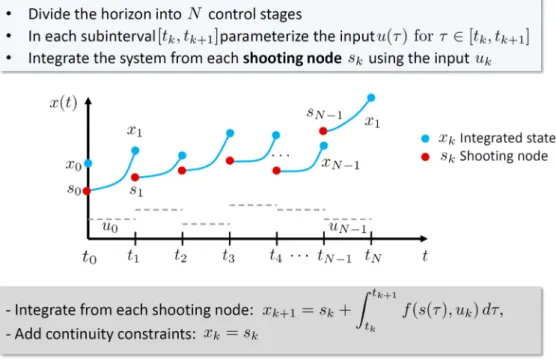
In order to get an NLP from the above problem, the dynamic problem needs to be parameterized. An option is to solve the optimization iteratively by a sequential approach, where the independent de-grees of freedom of 6 are discretized. Then an optimization problem with respect to these decision variables is setup, connected to a dynamic simulator where the differential equation set is solved numerically over the time window in order to compute the cost function and constraints. The so-called single-shooting approaches belong to this type. An alternative is using a simultaneous ap-proach, where the states trajectories are also split in discrete intervals whose starting point (initial guess) is decision variable for the optimizer. In this way, multiple integrations are run simultaneously and the task of linking the end of each interval with the initial point of the next one is left for the optimizer [9]. Figure 4 below gives an overview of this approach.
Figure 4: Simultaneous mul ple-shoo ng approach.
4.1.2
Input-deviation penalty
The formulation 5 - 8 explicitly parameterizes the input variables 𝑢 𝑡 ∈ ℝ along time, resulting in a large number of decision variables 𝑢 ∈ ℝ . In order to reduce the problem size, thinking in real-time DDR applications, it can be assumed that input measurements do not suffer of random errors but only of a possible systematic deviation Δ𝑢. Hence, instead of reconciling 𝑢 ∈ ℝ varia-bles, we significantly reduce the set to Δ𝑢 ∈ ℝ at the price of reducing the degrees of freedom. Thus, the DDR problem 5 - 8 reduces to:
minimize 𝑥, Δ𝑢, 𝑝̂ 𝐽 𝛾
𝜎 ⋅ 𝑦 𝑡 𝑦 𝑡
𝛾
𝜎 ⋅ Δ𝑢 9
subject to: 𝑑𝑥
𝑑𝑡 Ψ 𝑥, 𝑢, 𝑝̂ 0 𝑖: 1, … , 𝑛; 𝑢 𝑢 Δ𝑢; 10 ℎ 𝑥, 𝑢, 𝑝̂ 0 𝑗: 1, … , 𝑟; 𝑔 𝑥, 𝑢 0 𝑘: 1, … , 𝑚; 11
𝑦
𝐶 ⋅ 𝑥, 𝑢 ; Δ𝑈
Δ𝑢
Δ𝑈
;
𝑃
𝑝̂
𝑃
12
4.1.3
Moving-horizon window
A moving time window approach is useful to decrease the size of the discretized optimization problem. Therefore, it is important to choose an appropriate horizon length 𝐻: considering a large historical is very computationally demanding, so real-time constraints may not be satis-fied, but if 𝐻 is too small, the information available may not be enough to capture the dynam-ics, therefore to perform a sensible reconciliation.
The algorithm for moving-horizon DDR can be summarized in the following steps [11]: 1. Acquire process measurements at current time 𝑡 𝑡
2. Minimize 5 , under the constraints 6 - 7 over the time window 𝑡 𝐻 1 𝑇
𝑡 𝑡 , being 𝑇 𝑡 𝑡 the data sampling time.
3. Save 𝑥 at time 𝑡 as the reconciled signal for online control purposes 4. Repeat at the next time sample, 𝑡 𝑇
One advantage of the moving window approach is that the only tuning parameter is the size of the history horizon 𝐻, if the weights 𝛾 in 5 are equal.
At this point is where DDR shares several features with other online estimation techniques such as moving-horizon estimation (also involving model-based optimization) [12] or augment-ed Kalman filters [13].
4.1.4
Adaptive noise model
4.2
Enhanced formulation
The main obstacle of data reconciliation in industrial applications is the scarce number of available sensors that can provide an acceptable level of redundancy in the recorded data. This lack of redun-dancy leads to a model that is only able to calculate the system unknowns, using perhaps wrong measurements that cause the generation of erroneous solutions. In order to palliate this issue, two lines of action are explored: 1) artificially increasing the system redundancy and 2) mitigating the influence of gross errors in sensor measurements. The second one is later treated in Section 4.3, whereas an enhanced DDR formulation to increase redundancy is presented next.
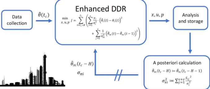
The main idea behind this method is to increase the system redundancy by adding a set of “virtual” measurements 𝜃 ∈ ℝ that are not directly sampled by sensors but that are initially guessed and later reconciled, since they are treated as normal measurements [15]. These virtual quantities 𝜃 can be either slow-varying variables or constant parameters and their previous reconciled values 𝜃 are “re-injected” into the DDR problem at each time instant together with the corresponding a posteriori variance 𝜎 [16]. Following this idea, the enhanced DDR problem from 5 - 8 can be mathematical-ly expressed as follows:
minimize 𝑥, 𝑢, 𝑝̂ 𝐽 𝛾
𝜎 ⋅ 𝜃 𝑡 𝜃 𝑡
𝛾
𝜎 𝜃 𝑡 𝜃 𝑡 1 13
subject to: 𝑑𝑥
𝑑𝑡 Ψ 𝑥, 𝑢, 𝑝̂ 0 𝑖: 1, … , 𝑛 14
ℎ 𝑥, 𝑢, 𝑝̂ 0 𝑗: 1, … , 𝑟; 𝑔 𝑥, 𝑢, 𝑝̂ 0 𝑘: 1, … , 𝑚 15
𝜃 𝑡
𝐶 ⋅ 𝑥, 𝑢 ; 𝑈
𝑢
𝑈
;
𝑃
𝑝̂
𝑃
16
With the assumption that the true values of the re-injected virtual variables remain almost constant between consecutive samples. Under this assumption, the following relations are employed to up-date these variables for the next DDR execution:
𝜃 𝑡 𝐻 ≔ 𝜃 𝑡 𝐻 1 ; 𝜎 ≔ 𝑆
𝜎 17
where 𝑆 is the sensitivity matrix2. Figure 3 below summarizes the enhanced DDR procedure.
Figure 5: Flow chart for the enhanced DDR execu on.
4.3
Treatment of gross errors
One of the issues of the data reconciliation based on a classical least-squares (LS) objective function is that the approach assumes that sensor measurements are affected by Gaussian noise with zero mean. However, this LS function is very affected by gross errors (i.e., systematic deviations from the expected coherent values) so the algorithm tries to spread these gross errors among all variables, thus distorting the estimations for the correct measurements. There are several approaches for deal-ing with gross errors in the literature, but only a few of them are practical for online DDR of industrial use. The policy summarized below intends to mitigate such gross-error effect by using robust estima-tors (also called M-estimators) [17] that are less sensitive to deviations from ideal Gaussian distribu-tions.
The basic idea is to look at the bulk of measurements and limit the weight of variables affected by gross errors [18]. In contrast to classical weighted least-squares 5 or 13 , which give quadratic importance to the errors, the robust estimators limit their contribution to the cost function when the error is large. In this way, the effect of the gross error is attenuated and the optimizer does not try to distribute the error among all the variables in order to avoid this high quadratic penalty.
There are some suitable robust estimators proposed in the literature like, for instance:
Welsch 𝑐
2 1 𝑒 18
Fair 𝑐 |𝑟 |
𝑐 log 1 |𝑟 |
𝑐 19
Where 𝑟 stands for the estimation error and 𝑐 is a user-defined parameter to tune the slope of the function. Among them, the Fair estimator has been chosen as the more suitable for practical large-scale implementations, because it is continuous (required for gradient-based nonlinear programming algorithms) and it gives a good tradeoff between complexity and performance (see Figure 6) [19].
Figure 6: Least squares and M-func ons represented for a range of values of the measurement error 𝒓𝒊.
5
Case study: Multiple-effect evaporation plant
One of the biggest evaporation plants at Lenzing AG is chosen as proof of concept for the DDR methods summarized in this report. This plant gives service attached to the fiber-production process and its goal is to regenerate an acid flow coming from the spinning process, where fibers take form from the previously processed cellulose pulp.
5.1
System description & modelling
The Lenzing evaporation plant considered for this report is basically formed by several evapo-ration chambers and heat exchangers arranged in serial connection, a steam condenser and a cooling system. Figure 7 depicts a simplified scheme of the line, in which some single equip-ment (evaporation chambers and exchangers) have been lumped due to lack of measureequip-ments in between them.
Figure 7: Simplified diagram of the evapora on plant with loca on of existent instrumenta on: transducers (blue) and controllers (green).
evaporation phase is performed in the last set of chambers 𝑉 thanks to the condenser, which sucks out steam by condensing it with cold water from a cooling tower. Finally, part of the concentrated liquid leaves the process and the rest mixes with the input, being recirculated through the process. A nonlinear steady-state model of this system (whose core part is based in first principles) was previ-ously developed for real-time optimization purposes [21]. The model equations are omitted for brev-ity (see the above reference for details) but can be summarized as follows :
Equations of energy and mass balances taken in the evaporators 𝑉 , 𝑉, heat exchangers
𝑊 , 𝑊, steam condensers, steam saturator and in the cooling tower.
Density relationships between mass and volumetric flows of the liquid mixture, water and steam as a function of temperature and/or pressure.
Heat transmission between fluids in the exchangers: 𝑄 𝑈𝐴 𝐿𝑀𝑇𝐷, where 𝑄 is the transmitted heat, 𝑈𝐴 is the heat-transmission coefficient (to be estimated), and the loga-rithmic mean temperature difference (𝐿𝑀𝑇𝐷) has been computed using the Chen's approx-imation [22].
Phase equilibriums in the evaporation chambers as a function of temperatures, pressure and concentrations.
Psychometric conditions in the cooling tower and experimentally obtained cooling perfor-mance depending on the temperature difference of the cool water with the ambient.
Relationship between the airflow through the cooling tower with the fan speed, including the experimentally identified convection effect due to in-out temperature difference.
In order to perform DDR, approximate first-order dynamics are added to the energy balances in the evaporation chambers, steam condensers and the cooling tower, trying to represent the energy ac-cumulation due to the fluids residence time in such equipment :
𝑚 ⋅ 𝑐 𝑑𝑇
𝑑𝑡 𝐹 ⋅ 𝐻 𝑇 , 𝐶 , 𝑃 𝐹 ⋅ 𝐻 𝑇 , 𝐶 , 𝑃 20
Where, simplifying a lot for brevity, 𝐹 and 𝐹 represent the inlet and outlet mass flows with their respective stream features (temperature, concentration and pressure), 𝐻 ⋅ states for the specific enthalpy function, 𝑚 is the total mass inside the equipment, 𝑐 represents the specific heat and 𝑇 can be the average or outlet temperature of the medium where the energy is accumulated. Normal-ly, the dominant dynamics in these equipment is the one of the liquid phase, so we choose the mass
𝑚, specific heat 𝑐 and temperature 𝑇 accordingly. Of course the concentrations and absolute mass of the liquid inside an equipment can vary with time too, but we neglected adding such dynamics in the mass balances because: a) it is faster than the one on the temperature and/or b) concentrations are not measured, so such dynamics cannot be checked.
Indeed, 𝑚 ⋅ 𝑐 can be lumped in a time constant 𝜏 and treated as a time-varying parameter to be estimated via enhanced DDR (Section 4.2).
5.2
Reconciliation results
1000 1200 1400 1600 1800 2000 2200 2400 Sample nº 105 110 115 120 125 130 135 ºC
W2 Saturated steam temperature
Reconciled Measured
The system dynamics has been discretized by orthogonal collocation [10] using 2-degree interpolat-ing polynomials. A movinterpolat-ing time-window of 𝐻 7 (corresponding to 35 min.) and the input-deviation approach (Section 4.1.2) are employed to define an enhanced DDR schema (Section 4.2). Some ob-tained results are presented and discussed below.
5.2.1
Example of gross-error detection
A selected reconciliation window of a week of operation is shown in Figure 8, where the measure-ments for the circulating flow of acid bath and the temperature of the saturated steam before enter-ing 𝑊 heat exchangers are depicted, together with its reconciled values obtained from DDR.
At the beginning, it can be observed that some biases between the reconciled and measured values appear from time to time, especially in what seems the plant is near to steady state. This could be because the plant model in steady state is not perfect or some corrupted data affected the parame-ter estimation. Nevertheless, this is not considered a big issue, as these biases eventually reduce to acceptable values.
Nonetheless, note that, since the sixth day onwards, a systematic error is detected in the steam tem-perature: indeed this error is not constant but seems to increase with the time. However, no sensible deviation is observed in the circulating flow. This is a clear indicator of that something has happened around the last stage of heat exchangers: it could be a gross error in the measurement due to a fault in the temperature sensor, or a physical change in the process (equipment fault or operation mode). It would be desirable to cross data with the maintenance historian to elucidate the origin of this error and, in case of online DDR, it would be recommendable to send a maintenance order to check the state of such sensor if the problem persists in time.
Figure 8: DDR execu on during 8 days of opera on.
1000 1200 1400 1600 1800 2000 2200 2400
5.2.2
Performance during transients
In order to evaluate the performance during transient behavior, a train of setpoint changes in the circulating flow and control temperature was scheduled in the plant, see Figure 9 and Figure 10. Some deviations between the measurements and the reconciled inputs can be observed just after some setpoint changes, especially in the circulating flow. This can be an indicator that we considered some slow dynamics in the model but they are faster in the real plant, so the estimated inputs by DDR are modified to fit the rest of the plant measurements. It could be also possible due to neglect-ing the sensors dynamics which, sometimes, might be important.
1300 1400 1500 1600 1700 1800 1900 2000 2100 2200 2300 2400
Sample nº
130 140 150 160 170 180 190 200 210 220
m
3 h
Circulating flow
Reconciled Measured
Figure 9: Induced changes in the circula ng flow (control input).
1300 1400 1500 1600 1700 1800 1900 2000 2100 2200 2300 2400
Sample nº
90 92 94 96 98 100 102 104 106 108 110
ºC
Bath control temperature
Reconciled Measured
Figures 11 to 13 below show the reconciled values or some intermediate temperatures in the plant, for which we have measurements to compare. In general, the obtained estimates are spikier than the corresponding measurements, which could be again a problem of plant-model mismatch in our simple approximations of the system dynamics, or just a smoothing effect by the sensors due to their own dynamics (normally temperature sensors act as a low-pass filter).
Special mention needs to be done for Figure 11. There, a recurrent gap of about 2 degree C is ob-served between the reconciled values and the measurements. This may indicate a problem in our model with the steady-state equations in equipment around the acid-bath inlet, or an indicator of that this sensor needs recalibration.
1300 1400 1500 1600 1700 1800 1900 2000 2100 2200 2300 2400
Sample nº
20 22 24 26 28 30 32 34 36 38 40
ºC
W1 spinbath inlet temperature
Reconciled Measured
Figure 11: Variability in the temperature inlet of the bath recircula on.
1300 1400 1500 1600 1700 1800 1900 2000 2100 2200 2300 2400
Sample nº
76 78 80 82 84 86 88 90 92
ºC
W1 spinbath outlet temperature
Reconciled Measured
1300 1400 1500 1600 1700 1800 1900 2000 2100 2200 2300 2400
Sample nº
95 100 105 110 115 120 125 130
ºC
W2 Saturated fresh steam temperature
Reconciled Measured
Figure 13: Temperature of the saturated steam at the 𝑾𝟐 inlet.
5.3
Time-varying parameter estimation
Apart from obtaining estimations for the model variables that are unmeasured, parameter estima-tions are provided by DDR as a byproduct. Among these, especially interesting are the estimaestima-tions for slow-varying parameters, because they represent indeed the long-term dynamics which has not been considered initially in the model, such as fouling, degradation, catalyst deactivation, etc. This kind of dynamics is normally very difficult to model by first principles for a particular system: there are several influencing factors and the underlying physics is complex. Hence, estimations provided by DDR can serve as “soft sensors” from which data-driven equations can be obtained by regression or pattern identification among other known variables.
This is the case in the Lenzing evaporation plant, where the plant efficiency decreases with time due to progressive fouling in the heat exchanger sets 𝑊 and 𝑊. The fouling effect can be observed indi-rectly as an increase of the specific steam consumption (measurement) over a month of operation, or directly by the evolution of the heat-transmission coefficients 𝑈𝐴 (unmeasured). Therefore, we have run enhanced DDR in the test data considering the coefficients 𝑈𝐴 for 𝑊 and 𝑊 as parame-ters to be estimated. The results over a week of operation are displayed in Figure 14.
Although the estimation is not very smooth (typical behavior when estimating this kind of coeffi-cients from noisy measurements) we can clearly observe a correlation between 𝑈𝐴 with respect to the circulating flow. This effect is coherent with the physics, as the heat transfer by convection is expected to increase with the flow (and vice versa).
0 500 1000 1500 2000 2500
Sample nº
130 140 150 160 170 180 190 200 210 220
m
3 /h
Circulating flow
Reconciled Measured
(a) Induced changes in the circula ng flow.
0 500 1000 1500 2000 2500
Sample nº
500 600 700 800 900 1000 1100
Jm
/K
Heat transmission coefficient
(b) Evolu on of the heat-transmission coefficient.
6
Concluding remarks
This deliverable has summarized the main ideas on dynamic data reconciliation to be applied in large-scale systems, putting special emphasis in allowing online implementations. In this way, the more suitable theoretical approaches have been reviewed and some have been tested in the multiple-effect evaporation plant of Lenzing AG.
As a first attempt, the obtained results were satisfactory enough to proof the DDR concepts in a large system. Nevertheless, the application of DDR to large processing plants has demonstrated to be challenging both from the theoretical and implementation aspects. One of the main difficulties encountered is related to the modelling : a representative dynamic model of the plant is required as a starting point to really trust DDR results, but large plants involve several complex processes difficult to model, even in steady state.
7
References
[1] M. Kujanpää, J. Hakala, T. Pajula, B. Beisheim, S. Krämer, D. Ackershott, M. Kalliski, S. Engell, U. Enste and J. L. Pitarch, Successful Resource Efficiency Indicators for process industries, vol. 290, Espoo: VTT Technology, 2017, p. 78.
[2] P. Kadlec, B. Gabrys and S. Strandt, "Data-driven Soft Sensors in the process industry,"
Computers & Chemical Engineering, vol. 33, no. 4, pp. 795-814, 2009.
[3] M. Leibman, T. Edgar and L. Lasdon, "Effcient data reconciliation and estimation for dynamic processes using nonlinear programming techniques," Computers & Chemical Engineering, vol. 16, pp. 963-986, 1992.
[4] N. Shrowti, K. Vilankar and R. Rhinehart, "Type-II Critical Values for a Steady-State Identifier,"
Journal of Process Control, vol. 20, no. 7, pp. 885-890, 2010.
[5] T. Huang, Steady State and Transient State Identification in an Industrial Process, MS Thesis. Oklahoma State University, 2013.
[6] R. Rhinehart, M. Su and U. Manimegalai-Sridhar, "Leapfrogging and Synoptic Leapfrogging: a new optimization approach," Computers and Chemical Engineering, vol. 40, pp. 67-81, 2012. [7] R. Rhinehart, "Automated Steady and Transient State Identification in Noisy Processes," in
American Control Conference (ACC), Washington, DC, USA, 2013.
[8] J. Taylor and M. Laylabadi, "A novel adaptive nonlinear dynamic data reconciliation and gross error detection method," in IEEE Conf. on Control Applications, Munich, 2006.
[9] H. Bock, M. Diehl, D. Leineweber and J. Schlöder, "A Direct Multiple Shooting Method for Real-Time Optimization of Nonlinear DAE Processes," in Nonlinear Model Predictive Control, F. Allgöwer and A. Zheng, Eds., Basel, Springer, 2000, pp. 245-267.
[10] L. T. Biegler, A. M. Cervantes and A. Wächter, "Advances in simultaneous strategies for dynamic process optimization," Chemical Engineering Science, vol. 57, no. 4, pp. 575-593, 2002.
[11] J. Taylor and R. Moreno, "Nonlinear Dynamic Data Reconciliation: In-depth Case Study," in IEEE Inter. Conf. on Control Applications (CCA), Hyderabad, 2013.
[12] V. M. Zavala, C. D. Laird and L. T. Biegler, "A fast moving horizon estimation algorithm based on nonlinear programming sensitivity," Journal of Process Control, vol. 18, no. 4, pp. 876-884, 2008. [13] S. Bai, J. Thibault and D. D. McLean, "Dynamic data reconciliation: Alternative to Kalman filter,"
Journal of Process Control, vol. 16, pp. 485-498, 2006.
[14] J. Taylor, "Statistical performance analysis of nonlinear stochastic systems by the monte carlo method," Trans. on Mathematics and Computers in Simulation, vol. 23, no. 1, pp. 21-33, 1981. [15] M. Bendig, Integration of Organic Rankine Cycles for Waste Heat Recovery in Industrial
[16] G. Heyen, E. Maréchal and B. Kalitventzeff, "Sensitivity calculations and variance analysis in plant measurement reconciliation," Computers & Chemical Engineering, vol. 20, no. S1, pp. S539-S544, 1996.
[17] P. Huber, "Robust statistics," in International Encyclopedia of Statistical Science, M. Lovric, Ed., Springer Berlin, 2014, pp. 1248-1251.
[18] N. Arora and L. Biegler, "Redescending estimators for Data Reconciliation and Parameter Estimation," Computers & Chemical Engineering, vol. 25, no. 11-12, p. 1585–1599, 2001.
[19] G. Shevlyakov, S. Morgenthaler and A. Shurygin, "Redescending M-estimators," Journal of Statistical Planning and Inference, vol. 138, pp. 2906-2917, 2008.
[20] M. Fuente, G. Gutierrez, E. Gomez, D. Sarabia and C. de Prada, "Gross error management in data reconciliation," in 9th International Symposium on Advanced Control of Chemical Processes, Whistler, British Columbia, Canada, 2015.
[21] J. L. Pitarch, C. G. Palacín, C. de Prada, B. Voglauer and G. Seyfriedsberger, "Optimisation of the Resource Efficiency in an Industrial Evaporation System," Journal of Process Control, vol. 56, pp. 1-12, 2017.
[22] J. J. J. Chen, "Comments on improvements on a replacement for the logarithmic mean,"