Avoiding order reduction when integrating linear
initial boundary value problems with exponential
splitting methods
I. Alonso-Mallo
∗, B. Cano
†IMUVA, Departamento de Matem´atica Aplicada,
Facultad de Ciencias, Universidad de Valladolid,
Paseo de Bel´en 7, 47011 Valladolid,
Spain
and
N. Reguera
‡IMUVA, Departamento de Matem´aticas y Computaci´on,
Escuela Polit´ecnica Superior, Universidad de Burgos,
Avda. Cantabria, 09006 Burgos,
Spain
Abstract
It is well known the order reduction phenomenon which arises when expo-nential methods are used to integrate in time initial boundary value problems, so that the classical order of these methods is reduced. In particular, this sub-ject has been recently studied for Lie-Trotter and Strang exponential splitting methods, and the order observed in practice has been exactly calculated. In this paper, a technique is suggested to avoid that order reduction. We deal directly with non-homogeneous time-dependent boundary conditions, without having to reduce the problem to homogeneous ones. We give a thorough error analysis of the full discretization and justify why the computational cost of the technique is negligible in comparison with the rest of the calculations of the method. Some numerical results for dimension splittings are shown which corroborate that much more accuracy is achieved.
∗Email: [email protected]
1
Introduction
Splitting methods are well known to be of interest for differential problems in which the numerical integration of separated parts of the equation is much easier or cheaper than the numerical integration as a whole [14, 22]. Moreover, if the stiff part of those sepa-rated problems is linear, it can be solved in an explicit way by using exponential-type methods without showing stability problems. This makes exponential splitting meth-ods very much suitable for the numerical integration of partial differential equations and, in particular, for multidimensional problems in simple domains, where considering alternatively each direction of the differential operator leads to simpler integrators.
In [12], a thorough analysis is given for the classical-1st-order Lie-Trotter and classical-2nd-order Strang exponential methods when integrating linear initial bound-ary value parabolic problems under homogeneous Dirichlet boundbound-ary conditions. The general conclusion there is that order reduction to 1 appears for the local error with Lie-Trotter method although there is no order reduction for the global one. With Strang method, order reduction to 1 for the global error is shown. When the boundary condition is not homogeneous but it is the restriction of a known smooth function on the total domain, the problem can be reduced to one in which the boundary condition is homogeneous, but in which the source term contains derivatives of that smooth func-tion, which must be calculated. In any case, the previous mentioned order reduction would turn up.
Our aim in this paper is to approximate regular solutions of linear differential problems with generalizations of Lie-Trotter and Strang methods which avoid com-pletely order reduction. Moreover, we will deal directly with non-homogeneous and time-dependent boundary conditions. We will give a technique to do it which requires a computational cost which is negligible compared with the total cost of the method since it just adds calculations with grid values on the boundaries, and not with the num-ber of grid values on the total domain. In this sense, the technique is as cheap as that suggested in [4] for exponential Lawson methods and, among others, in [1, 2] for other standard Runge-Kutta type methods. The idea, in a similar way as in [8, 16, 17], is to consider suitable intermediate boundary conditions for the split evolutionary problems. The main difference with [16, 17] is that they just consider there the one-dimensional first-order in time hyperbolic problem where one of the splitting parts is assumed to be smooth (or vary slowly) and the suggestion of the intermediate boundary conditions is very much based on a particular space discretization. As distinct, in the present paper both the problem and the space discretization are much more general. As for [8], although the problem is more general than in [16, 17], numerical differentiation is required to approximate the boundary conditions of the intermediate evolutionary problems, while here they are given directly in terms of data. Besides, as we consider exponential methods and we use exact boundary values, no stability requirement is needed and, as final differences, not only the class of linear problems is more general here but also thethe way to measure the error in the analysis is more standard.
discretization for each part of the differential operator splitting. This is important, not only because in practice a space discretization is necessary and therefore the errors which come from space must be controlled, but also because the complete description of the suggested method must be given to those who are just interested in applying the method and not on the analysis. More particularly, we consider spatial schemes satisfying quite general hypotheses, which include for example simple finite-differences or collocation spectral methods. Moreover, the exact formulas which must be imple-mented after full discretization to avoid order reduction in the local and global error are given in (36)-(38) for Lie-Trotter and in (50)-(54) for Strang method. In Section 8.1, we justify that, for dimension splittings, the terms corresponding to the boundary in those formulas can always be calculated in terms of the data of the problem for Lie-Trotter method and, when the splitting terms of the differential operator commute, also for Strang method. Nevertheless, for the latter integrator, when the splitting operators do not commute, we offer the alternative (54)-(58), which boundaries can always be calculated in terms of data. In such a way, just order 2 instead of 3 is obtained for the local error but, in any case, no order reduction is shown for the global error in practice. Although it is not an aim of this paper, there are already results on applying a similar technique to nonlinear problems [5, 7], and [11] tries to compare with the technique in [9, 10] for them.
The paper is structured as follows. Section 2 gives some preliminaries on the ab-stract formulation of the problem and the definition of the time integrators. Then, the technique to avoid order reduction after time discretization with Lie-Trotter method is described in Section 3, as well as the analysis on the local error. Section 4 does the same for Strang method. In Section 5, the hypotheses on the spatial discretization are stated. Sections 6 and 7 describe the formulas for the implementation after full discretization for Lie-Trotter and Strang methods respectively, and the local and global errors are then analysed. Finally, in Section 8, it is justified that the dimension split-ting problem fits into the abstract framework, that the information which is needed on the boundary can be calculated from data and some numerical results are given which corroborate the results of previous sections.
2
Preliminaries
Let X and Y be Banach spaces and let L : D(L) → X and ∂ : D(L) → Y be linear operators. Our goal is to study full discretizations of the linear abstract inhomogeneous initial boundary value problem
u′(t) = Lu(t) +f(t), 0≤t≤T, u(0) = u0 ∈X,
∂u(t) = g(t)∈Y, 0≤t≤T.
(1)
(i) The boundary operator ∂ :D(L)⊂X →Y is onto.
(ii) Ker(∂) is dense in X and L0 : D(L0) = ker(∂) ⊂ X → X, the restriction of L
to Ker(∂), is the infinitesimal generator of aC0-semigroup{etL0}t≥0 inX, which
type ω is assumed to be negative.
(iii) If λ∈C satisfies Re(λ)> ω and v ∈Y, then the steady state problem
Lx = λx, (2)
∂x = v,
possesses a unique solution denoted byx=K(λ)v. Moreover, the linear operator K(λ) :Y →D(L) satisfies
∥K(λ)v∥X ≤M∥v∥Y,
where the constant M holds for any λ such that Re(λ)≥ω0 > ω.
The main goal of this work is to propose a suitable generalization, for initial bound-ary value problems, of two popular exponential splitting time integrators, the Lie-Trotter and the Strang methods. Therefore, we suppose that
L=A+B, (3)
where A : D(A) → X and B : D(B) → X are linear operators which are assumed to be simpler than L in some sense, and D(L) ⊆ D(A)∩ D(B). We also suppose that, for some Banach spaces YA and YB, the linear operators ∂A : D(A) → YA and ∂B :D(B)→YB satisfy the following assumptions:
(A1) Ker(∂) = Ker(∂A)∩Ker(∂B).
(A2) A0 : Ker(∂A) ⊂X → X and B0 :D(B0) = Ker(∂B) ⊂ X →X, the restrictions
of A (resp. B) to Ker(∂A) (resp. Ker(∂B)), are the infinitesimal generators of C0- semigroups in X: {etA0}t≥0, with type ωA, and {etB0}t≥0, with type ωB. We assume that max(ωA, ωB)<0.
(A3) If λ ∈ C satisfies Re(λ) >max(ωA, ωB) and vA ∈ YA, vB ∈ YB, then the steady state problems
Ax = λx, ∂Ax = vA,
By = λy, ∂Bx = vB,
(4)
possess unique solutions denoted by x = KA(λ)vA, y = KB(λ)vB. Moreover, these operators KA(λ) :YA→D(A), KB(λ) :YB →D(B), satisfy
∥KA(λ)vA∥X ≤LA∥vA∥YA, ∥KB(λ)vA∥X ≤LB∥vB∥YB, (5)
In order to define the time integrators which are used in this paper, we will consider initial boundary value problems which can be written as
u′(s) = Au(s), u(0) = u0,
∂Au(s) = v0+v1s+v2s2,
(6)
whereu0 ∈X andv0, v1, v2 ∈YA(Similar problems withB instead ofAare also used.).
The study of the well posedness of these problems is not the objective of this paper but, when the initial value is regular and compatible with the boundary datum at s = 0, we can explicitly obtain the solution by using the hypotheses (A2) and (A3).
Lemma 1. [3, 20] If f ∈C1([0, T], X), then ∫t
0 e
sA0f(t−s)ds ∈D(A
0) and
A0
∫ t
0
esA0f(t−s)ds=etA0f(0)−f(t) +
∫ t
0
esA0f′(t−s)ds,
for t≥0.
Proposition 2. Assume that u0 ∈ D(A) and ∂Au0 = v0, then the solution of (6) is
given by
u(t) = etA0(u
0−KA(0)v0) +KA(0)(v0+v1t+v2t2) (7)
−
∫ t
0
esA0K
A(0)(v1+ 2v2(t−s))ds.
Proof. Since ∂Au0 =v0, u0−KA(0)v0 ∈D(A0) and therefore
∂A
(
etA0(u
0−KA(0)v0)
)
= 0.
On the other hand, from Lemma 1,
∂A
(∫ t
0
esA0K
A(0)(v1+ 2v2(t−s))ds
)
= 0,
and we deduce that∂Au(t) =v0+v1t+v2t2. Moreover,
u′(t) =etA0A
0(u0−KA(0)v0) +KA(0)(v1+ 2v2t)−etA0KA(0)v1−
∫ t
0
esA0K
A(0)2v2ds.
On the other hand, by using Lemma 1 and the definition of KA(0),
Au(t) = etA0A
0(u0 −KA(0)v0)−A0
∫ t
0
esA0K
A(0)(v1 + 2v2(t−s))ds
= etA0A
0(u0 −KA(0)v0))−etA0KA(0)v1+KA(0)(v1+ 2v2t)−
∫ t
0
esA0K
A(0)2v2ds.
Remark 3. Notice that (7) is well defined for anyu0 ∈X andv0, v1, v2 ∈YA; therefore, it may be considered as a generalized solution of (6) which can be used even whenu0 is
not regular or not compatible with the boundary values. We will use this fact in order to establish the time integrator method in the following section.
Because of hypothesis (A2),{φj(tA0)}3j=1 and {φj(tB0)}3j=1 are bounded operators
for t > 0, where {φj} are the standard functions used in exponential methods [15], which are defined by
φj(tA0) =
1 tj
∫ t
0
e(t−τ)A0 τ
j−1
(j −1)!dτ, j ≥1, (8)
and can be calculated in a recursive way through the formulas
φj+1(z) =
φj(z)−1/j!
z , z ̸= 0, φj+1(0) = 1
(j+ 1)!, φ0(z) =e
z. (9)
These functions are well known to be bounded on the complex plane when Re(z)≤0. For the time integration, we will center on Lie-Trotter and Strang methods, which applied to a finite-dimensional linear problem like
U′(t) =M1U(t) +M2U(t) +F(t), (10)
whereM1 and M2 are matrices, are described by the following formulas at each step
Un+1 = ekM1ekM2
(
Un+kF(tn)
)
, (11)
Un+1 = e
k
2M1e
k
2M2(e
k
2M2e
k
2M1U
n+kF(tn+ k 2)
)
. (12)
wherek > 0 is time step size andtn=nk for n≥0.
For the study of the Lie-Trotter method, we also assume that the solution of (1) satisfies the following
(A4) For everyt∈[0, T], and for any natural numbersl1, l2, j such thatl1+l2+j ≤2,
u(j)(t)∈D(Al1Bl2) andAl1Bl2u(j)(t)∈C([0, T], X).
Remark 4. From the hypothesis (A4) and the formulas
u′ =Au+Bu+f, Au′ =A2u+ABu+Af, Bu′ =BAu+B2u+Bf,
we deduce thatf(t)∈D(A)∩D(B) for t∈[0, T] and f, Af, Bf ∈C([0, T], X).
For the finer results on Strang method, we assume that
(A4’) For every t∈[0, T], and for any natural numbers l1, l2, l3, l4, j such thatl1+l2+
l3+l4+j ≤3,u(j)(t)∈D(Al1Bl2Al3Bl4) and Al1Bl2Al3Bl4u(j)(t)∈C([0, T], X).
Remark 5. From the hypothesis (A4’) we deduce that f(t)∈D(A)∩D(B)∩D(A2)∩
Remark 6. Although the assumptions (A4) and (A4’) seem complicated, we emphasize that, in the context of partial differential problems, they only imply that the solution u(t) is regular enough in time and space.
We would like to clarify that, in the literature, A and B usually denote what we now call the operatorsA0 and B0 (which are the restriction of the present A and B to
the kernels of the boundary operators ∂A and ∂B). In such a case, hypotheses similar to (A4) and (A4’) are artificial since belonging to the domain of a power ofA0 (orB0)
implies vanishing conditions in the boundary which are not necessarily satisfied by the solution of (1). Because of that, order reduction turns up in the general case, and that is what we manage to avoid in the present paper.
3
Time semidiscretization: exponential Lie-Trotter
splitting
In this section, we give the technique to generalize the Lie-Trotter exponential method for the solution of initial boundary value problems with non-vanishing boundary condi-tions. Besides, we prove the full-order of the local error of the time semidiscretization, that is, the time order reduction is completely avoided.
3.1
Description of the technique
The technique which we suggest is based on the following:
When L0 is the infinitesimal generator of a C0-semigroup etL0, t ≥ 0, and u0 ∈
D(L0), the solution of the problem
u′(t) = L0u(t),
u(0) = u0, (13)
is given byu(t) = etL0u
0. In this way, we are able to use exponential methods when we
want to approximate the solution of an ordinary differential system and, in the case of a partial differential problem, we can approximate the solution of a pure initial value problem or an initial boundary value problem with homogeneous or periodic boundary values.
For unbounded operators which are not associated to vanishing boundary con-ditions, as those in (1), we mimic (13) by solving analogous differential problems where some boundaries must be specified. As we aim to generalize C0-semigroups,
for the boundaries we consider Taylor expansions until the order of accuracy we want to achieve. More precisely, considering, forχ=Aor χ=B, the notation ϕχ,η0,ηˆ(s) for
the solution of
η′(s) = χη(s), η(0) = η0,
we firstly consider
vn(s) =ϕB,un+kf(tn),vˆn(s), (15)
where
ˆ
vn(s) =u(tn) +kf(tn) +sBu(tn). (16)
Then, we take
wn(s) = ϕA,vn(k),wˆn(s) (17)
where
ˆ
wn(s) = u(tn) +kf(tn) +kBu(tn) +sAu(tn). (18)
(Notice that, althoughvn(s), ˆvn(s),wn(s) and ˆwn(s) do in fact depend onk, we do not include the parameterk as a subindex in order to simplify the notation.)
In such a way, the numerical method is given by
un+1 =wn(k). (19)
In practice, we need to calculate the boundary values∂Bˆvn(s) and∂Awn(s) in terms ofˆ data. In Section 8, we study how to calculate these boundary values taking hypothesis (A4) into account when the splitting is dimensional.
3.2
Local error of the time semidiscretization
In order to study the local error, we consider the value obtained in (19) starting from u(tn) instead of un. More precisely, we consider
un+1 =wn(k)
where wn(s) = ϕA,vn(k),wˆn(s) with ˆwn(s) that in (18), and vn(s) = ϕB,u(tn)+kf(tn),vˆn(s)
where ˆvn(s) is that in (16).
Before bounding the local error ρn+1 = ¯un+1 −u(tn+1), let us first study more
thoroughly wn(s) and vn(s).
Lemma 7. Under hypotheses (A1)-(A4),
vn(s) = u(tn) +kf(tn) +sBu(tn) +ksφ1(kB0)Bf(tn) +s2φ2(sB0)B2u(tn),
wn(s) = u(tn) +k(Bu(tn) +f(tn)) +sAu(tn) +k2esA0[φ1(kB0)Bf(tn) +φ2(kB0)B2u(tn)] +ksφ1(sA0)A(Bu(tn) +f(tn)) +s2φ2(sA0)A2u(tn),
Proof. Notice that
ˆ
v′n(s) = Bu(tn) =Bvn(s)ˆ −sB2u(tn)−kBf(tn). Therefore,
v′n(s)−ˆvn′(s) = B(vn(s)−ˆvn(s)) +sB2u(tn) +kBf(tn), vn(0)−vˆn(0) = 0,
∂B(vn(s)−vˆn(s)) = 0. Then,
vn(s) = ˆvn(s) +
∫ s
0
e(s−τ)B0[τ B2u(tn) +kBf(tn)]dτ
= u(tn) +kf(tn) +sBu(tn) +s2φ2(sB0)B2u(tn) +ksφ1(sB0)Bf(tn). On the other hand,
ˆ
w′n(s) = Au(tn) =Awn(s)ˆ −kAf(tn)−kABu(tn)−sA2u(tn), ˆ
wn(0) = u(tn) +kBu(tn) +kf(tn).
Therefore,
w′n(s)−wˆn′(s) = A(wn(s)−wˆn(s)) +kAf(tn) +kABu(tn) +sA2u(tn), wn(0)−wn(0) =ˆ k2φ2(kB0)B2u(tn) +k2φ1(kB0)Bf(tn),
∂A(wn(s)−wˆn(s)) = 0,
from what
wn(s)−wˆn(s) = k2esA0[φ2(kB0)B2u(tn) +φ1(kB0)Bf(tn)] +
∫ s
0
e(s−τ)A0[kA(Bu(t
n) +f(tn)) +τ A2u(tn)]dτ, which proves the lemma taking the definition (8) of φ1 and φ2 into account .
¿From this, we deduce the full order of consistency.
Theorem 8. Under assumptions (A1)-(A4), when integrating (1) along with (3) with
Lie-Trotter method using (19), the local error satisfies
ρn+1 ≡un+1−u(tn+1) = O(k2).
Proof. By considering s=k in Lemma 7 and using (1), it is clear that
¯
un+1 = u(tn) +k[Bu(tn) +Au(tn) +f(tn)] +k2ekA0φ
2(kB0)B2u(tn) +k2φ1(kA0)ABu(tn) +k2φ2(kA0)A2u(tn) +k2ekA0φ
4
Time semidiscretization: exponential Strang
split-ting
With the same idea as in Section 3, we describe now how to generalize Strang expo-nential method to initial boundary value problems with nonvanishing boundary values in such a way that time order reduction is completely avoided.
4.1
Description of the technique
For the time integration of (1) along with (3), we firstly consider
vn(s) =ϕA,un,bvn(s) (20)
where
b
vn(s) =u(tn) +sAu(tn) + s2
2A
2
u(tn); (21)
secondly,
wn(s) =ϕB,vn(k2),wbn(s) (22)
where
b
wn(s) = u(tn) + k
2Au(tn) + k2
8 A
2u(t
n) +sBu(tn) +s k
2BAu(tn) + s2
2B
2u(t
n);(23) thirdly,
rn(s) = ϕB,wn(k2)+kf(tn+k2),rbn(s), (24)
where
b
rn(s) = u(tn) + k
2Au(tn) + k
2Bu(tn) +kf(tn+ k 2) +k 2 8 A 2u(t
n) + k2
4BAu(tn) + k2
8B
2u(t
n)
+sBu(tn) +s k
2BAu(tn) +s k 2B
2u(t
n) +skBf(tn+ k 2) +
s2 2B
2u(t
n); (25) and, finally,
zn(s) =ϕA,rn(k2),bzn(s) (26)
where
b
zn(s) = u(tn) + k
2Au(tn) +kBu(tn) +kf(tn+ k 2) +k 2 8A 2u(t
n) + k2
2 BAu(tn) + k2
2 B
2u(t
n) + k2
2 Bf(tn+ k 2)
+sAu(tn) +sk 2A
2
u(tn) +skABu(tn) +skAf(tn+k 2) +
s2
2A
2
Then, we advance a step by taking
un+1 =zn( k
2). (28)
In practice, we need to calculate the boundary values in (20), (22), (24) and (26) in terms of dataf and g. In Section 8, we study how to calculate these boundary values taking hypothesis (A4’) into account when alternating directions are used.
4.2
Local error of the time semidiscretization
In order to study the local error, we consider the functionsvn,wn,rnand zn, obtained in (20), (22),(24),(26), starting fromun =u(tn) in (20). Following a similar argument as that of Lemma 7, this result follows:
Lemma 9. Under hypotheses (A1)-(A3) and (A4’),
vn(s) = ˆvn(s) +s3φ3(sA0)A3u(tn), wn(s) = wˆn(s) +
k3 8e
sB0φ
3(
k 2A0)A
3u(t
n) + k2
8 sφ1(sA0)BA
2u(t
n) + k 2s
2φ
2(sA0)B2Au(tn) +s3φ3(sA0)B3u(tn),
rn(s) = ˆrn(s)−esB0[ k3
8 e
k
2B0φ3(k
2A0)A
3u(t
n) + k3
16φ1( k
2A0)BA
2u(t
n)
+k
3
8φ2( k 2A0)B
2
Au(tn) + k3
8 φ3( k 2A0)B
3
u(tn)]
+sφ1(sB0)[
k2
4 B
2Au(t
n) + k2
8 B
3u(t
n)]
+s2φ2(sB0)[
k 2B
2Au(t
n) + k 2B
3u(t
n) +kB2f(tn+ k 2)] +s
3φ
3(sB0)B3u(tn),
zn(s) = zˆn(s)−esA0e
k
2B0[k
3
8e
k
2B0φ
3(
k 2A0)A
3u(t
n) + k3 16φ1(
k
2A0)BA
2u(t
n)
+k
3
8φ2( k 2A0)B
2Au(t
n) + k3
8 φ3( k 2A0)B
3u(t
n)]
+sk2φ1(sA0)[
1 8A
3u(t
n) + 1
2ABAu(tn) + 1 2AB
2u(t
n) + 1
2ABf(tn+ k 2)]
+s2kφ2(sA0)[
1 2A
3u(t
n) +A2Bu(tn) +A2f(tn+ k 2)] +s
3φ
3(sA0)A3u(tn).
From Lemma 9, it is clear that
zn( k
2) = bzn( k
2) +O(k
3)
= u(tn) +k(A+B)u(tn) +kf(tn)
+k
2
2
(
(A+B)2u(tn) + (A+B)f(tn) +f′(tn)
)
+O(k3)
= u(tn) +ku′(tn) + k
2
2 u
′′(tn) +O(k3
Then, if we define
un+1 =zn( k 2),
we have proved the following result:
Theorem 10. Under assumptions (A1)-(A3),(A4’), when integrating (1) along with
(3) with Strang method using the procedure (20)-(28), the local error satisfies
ρn+1 =u(tn+1)−un+1 =O(k3).
We will show in Section 8 that, when the splitting is dimensional, the terms of second order ins and k in the functions (21)-(23)-(25)-(27) can be calculated in terms of the data f and g only when the operators A and B commute. However, the alternative boundary values
b
vn(s) = u(tn) +sAu(tn),
b
wn(s) = u(tn) + k2Au(tn) +sBu(tn),
b
rn(s) = u(tn) + k2Au(tn) + k2Bu(tn) +kf(tn+ k2) +sBu(tn),
b
zn(s) = u(tn) + k2Au(tn) +kBu(tn) +kf(tn+k2) +sAu(tn),
(29)
can always be calculated and we obtain
Theorem 11. Under assumptions (A1)-(A4), when integrating (1) along with (3)
with Strang method using the technique (20),(22), (24), (26), (28), with the alternative boundary values (29), the local error satisfies
ρn+1 =u(tn+1)−un+1 =O(k2).
5
Spatial discretization
In this section, we describe a quite general procedure to discretize in space the corre-sponding evolutionary problems.
Although the previous analysis is valid for other types of boundary conditions, we consider here, for the sake of simplicity, an abstract spatial discretization which is suit-able for Dirichlet boundary conditions. (Look at [5] for a complete analysis of a similar technique with Neumann or Robin boundary conditions for nonlinear problems where the nonlinear part is a smooth operator. With linear problems, although both oper-ators are unbounded, the analysis there would be extended in a simpler way because the boundary conditions can always be exactly calculated in terms of data instead of just approximately, as it happens in [5].)
Without loss of generality, we will assume that we have the same parameter of space discretization forA andB. Let us denote it byh∈(0, h0]. LetXh be a family of finite dimensional spaces, approximatingX. The norm in Xh is denoted by ∥·∥h. We suppose that
in such a way that the internal approximation is collected in Xh,0 and Xh,b accounts for the boundary values.
The elements in D(A0)∩D(B0), which are regular in space and have vanishing
boundary conditions, can be approximated inXh,0. However, it is possible to consider
elementsu∈X which are regular in space but with non-vanishing boundary conditions, i.e. u∈D(A)∩D(B). Then, it is necessary to use the whole discrete spaceXh.
Since the solution is known at the boundary, our goal is to obtain a value in Xh,0
which is a good approximation inside the domain. Let us take a projection operator
Ph :X →Xh,0.
Whenx∈D(A0)∩D(B0),Phxwill be itsbest approximation inXh,0. We also assume
that there exist interpolation operators
Qh,A :YA→Xh,b, Qh,B :YB →Xh,b,
which permit to discretize spatially the boundary values.
On the other hand, the operators A and B are approximated by means of the operators
Ah :Xh →Xh,0, Bh :Xh →Xh,0,
in such a way thatAh,0 and Bh,0, the restrictions ofAh and Bh to the subspaces Xh,0,
are approximations ofA0 andB0. Therefore, whenxh =xh,0+xh,b ∈Xh,0⊕Xh,b =Xh, we have
Ahxh =Ah,0xh,0+Ahxh,b, Bhxh =Bh,0xh,0+Bhxh,b.
By using this, the following semidiscrete problem arises after discretising (1) along with (3) in space,
Uh′(t) = Ah,0Uh(t) +Bh,0Uh(t)
+AhQh,A∂Ag(t) +BhQh,B∂Bg(t) +Phf(t), Uh(0) = Phu(0).
(30)
The subsequent analysis is carried out under the following hypotheses, which are related to those in [4] (see also [6]).
(H1) The operators Ah,0 and Bh,0 are invertible and generate uniformly bounded C0
-semigroups etAh,0, etBh,0, on X
h,0 satisfying
||etAh,0||
h,||etBh,0||h ≤M, (31) where M ≥1 is a constant.
(H2) For each u∈X,vA∈YA and vB ∈YB, there exist constants C,CA′ and CB′ such that
(H3) We define the elliptic projections Rh,A :D(A) → Xh,0 and Rh,B :D(B) → Xh,0
as the solutions of
Ah(Rh,Au+Qh,A∂Au) = PhAu, Bh(Rh,Bu+Qh,B∂Bu) =PhBu. (33)
We assume that there exists a subspace Z of X, such that, for u∈Z,
(a) A−01u, B0−1u∈Z and etA0u, etB0u∈Z, for t≥0,
(b) for some εh,A and εh,B which are small withh,
∥Ah,0(Phu−Rh,Au)∥h ≤εh,A∥u∥Z, ∥Bh,0(Phu−Rh,Bu)∥h ≤εh,B∥u∥Z.
6
Full discretization: exponential Lie-Trotter
split-ting
Instead of integrating firstly in space (30) and then in time, which is the standard method of lines for the integration of (1), in this section we apply the space discretiza-tion to the intermediate evoludiscretiza-tionary problems which were described in Secdiscretiza-tion 3 when integrating firstly in time. In such a way, the following final formulas are obtained.
6.1
Final formula for the implementation
We apply the space discretization described above to the operators A and B which appear in the evolutionary problems (14) corresponding to (15) and (17) and we obtain Vh,n(s), Wh,n(s)∈Xh,0 as the solutions of
Vh,n′ (s) = Bh(Vh,n(s) +Qh,B∂Bˆvn(s)),
Vh,n(0) = Uh,n+kPhf(tn), (34)
where ˆvn(s) is that in (16), Uh,n∈Xh,0 is the numerical solution in the interior of the
domain after full discretization atn steps, and
Wh,n′ (s) = Ah(Wh,n(s) +Qh,A∂Awˆn(s)),
Wh,n(0) = Vh,n(k), (35)
where ˆwn(s) is that in (18). In such a way, by using the variations of constants formula,
Vh,n(k) = ekBh,0[Uh,n+kPhf(tn)] +
∫ k
0
e(k−s)Bh,0B
hQh,B∂B[u(tn) +kf(tn) +sBu(tn)]ds,
Wh,n(k) = ekAh,0Vh,n(k) +
∫ k
0
and, using then the definition of the functions φ1 and φ2 in (8),
Vh,n(k) =ekBh,0[Uh,n+kPhf(tn)] (36)
+k
[
φ1(kBh,0)BhQh,B∂B[u(tn) +kf(tn)] +kφ2(kBh,0)BhQh,B∂BBu(tn)
]
,
Wh,n(k) =ekAh,0Vh,n(k) (37)
+k
[
φ1(kAh,0)AhQh,A∂A[u(tn) +k(Bu(tn) +f(tn))] +kφ2(kAh,0)AhQh,A∂AAu(tn)
]
,
and the numerical solution at stepn+ 1 is therefore given by
Uh,n+1 =Wh,n(k). (38)
Moreover, we will take, as initial condition,
Uh,0 =Phu(0). (39)
Remark 12. Notice that, when
∂u(tn) =∂Au(tn) = ∂Bu(tn) = 0, (40)
it is also deduced from (1) along with (3) that∂f(tn) = 0. Therefore, formulas (36)-(37) just reduce to the standard time integration with Lie-Trotter method of the correspond-ing differential system
Uh′(t) = Ah,0Uh(t) +Bh,0(t)Uh(t) +Phf(t).
Although the order for the local error under these assumptions is not explicitly stated in [12], when the exact solution of (1) satisfies (40), we are implicitly proving that there is no order reduction in the local error with the standard Lie-Trotter method.
Remark 13.The calculation of the terms in (36) and (37) which contain the
exponential-type functionscan be performed with Krylov techniques in general [13] and with discrete sine transforms for some particular cases. In any case, we would like to notice that, for many space discretizations, forvA ∈YAand vB ∈YB, AhQh,AvA andBhQh,BvB are local in the sense that they vanish on the interior grid nodes (or great part of them). (See Section 8.) Because of this, for the terms which contain the functions φ1 and φ2, another possibility when the stepsize k is fixed during all integration is to calculate
once and for all at the very beginning just some columns of the matrices which represent φ1(kAh,0), φ2(kAh,0), φ1(kBh,0) and φ2(kBh,0). After that, at each step, just a linear
combination of those columns would be necessary. In practice, Ah,0 and Bh,0 can be
represented by block-diagonal matrices (where the blocks in the diagonal can even be the same in some cases, as when A+B is the Laplacian) and therefore, φ1 or φ2 over k
times those matrices is also block-diagonal. Due to that, the number of non-vanishing elements of each necessary column of φi(kAh,0) and φi(kBh,0) would just be O(J) if J
6.2
Local errors
In order to define the local error, we consider
Uh,n+1 =Wh,n(k), (41) whereWh,n(s) is the solution of
W′h,n(s) = Ah(Wh,n(s) +Qh,A∂Awn(s)),ˆ Wh,n(0) = Vh,n(k),
(42)
with ˆwn(s) that in (18) andVh,n(s) the solution of
V′h,n(s) = Bh(Vh,n(s) +Qh,B∂Bvˆn(s)),
Vh,n(0) = Ph[u(tn) +kf(tn)], (43)
with ˆvn(s) in (16). We now define the local error att =tn as
ρh,n =Phu(tn)−Uh,n,
and study its behaviour in the following theorem.
Theorem 14. Under assumptions (A1)-(A4) and (H1)-(H3), when integrating (1) with
Lie-Trotter method as described in (36),(37),(38),(39), whenever the functions in (A4) belong to the spaceZ which is introduced in (H3), the local error after full discretization satisfies
ρh,n+1 =O(kεh,A+kεh,B +k2),
where εh,A and εh,B are those in (H3b).
Proof. From the definition of ρh,n,
ρh,n+1 = (Phu(tn+1)−Phun+1) + (Phun+1−Uh,n+1)
= Phρn+1+ (Phwn(k)−Wh,n(k)).
Using Theorem 8 and (32), the first term in parenthesis is O(k2). In order to bound the second term, we apply the operator Ph to (14) (corresponding to wn(s)) and use (33),
Phw′n(s) = PhAwn(s)
= Ah(Rh,Awn(s) +Qh,A∂Awn(s))ˆ
= Ah,0Phwn(s) +Ah,0(Rh,A −Ph)wn(s) +AhQh,A∂Awˆn(s) Phwn(0) = Phvn(k).
Then, subtracting (42),
Phw′n(s)−W
′
Solving this problem exactly,
Phwn(k)−Wh,n(k) = ekAh,0(Phvn(k)−Vh,n(k)) (44)
+
∫ k
0
e(k−s)Ah,0A
h,0(Rh,A−Ph)wn(s)ds.
Making the difference now between (14) multiplied byPh (and corresponding tovn(s)) and (43),
Phv′n(s)−V
′
h,n(s) = Bh,0(Phvn(s)−Vh,n(s)) +Bh,0(Rh,B −Ph)vn(s), Phvn(0)−Vh,n(0) = 0,
which implies that
Phvn(k)−Vh,n(k) =
∫ k
0
e(k−s)Bh,0B
h,0(Rh,B−Ph)vn(s)ds =O(kεh,B),
due to (31) and (H3b) considering thatvn(s)∈Z because of Lemma 7, the hypotheses on u and f, (H3a) and the recursive definition of {φj}. Using this in (44) together with (31), (H3), and Lemma 7 again with wn(s) ∈ Z now, it follows that Phwn(k)− Wh,n(k) = O(kεh,A+kεh,B), which proves the result.
6.3
Global errors
We now study the global errors att=tn,
eh,n=Phu(tn)−Uh,n.
Theorem 15. Under the same assumptions of Theorem 14 and assuming also that
there exists a constantC such that, whenever nk∈[0, T],
∥(ekAh,0ekBh,0)n∥
h ≤C, (45)
the global error satisfies
eh,n =O(k+εh,A+εh,B),
where εh,A and εh,B are those in (H3b).
Proof. It suffices to notice that
eh,n+1 = [Phu(tn+1)−Uh,n+1] + [Uh,n+1−Uh,n+1] =ρh,n+1+Wh,n(k)−Wh,n(k),
where the definition of ρh,n+1, (38) and (41) have been used. Then, considering (34),
(35), (42) and (43),
and we obtain the recursive formula
eh,n+1 =ρh,n+1+ekAh,0ekBh,0eh,n. Sinceeh,0 = 0 because of (39), this implies that
eh,n = n
∑
l=1
(ekAh,0ekBh,0)n−lρ
h,l,
which, together with Theorem 14 and (45), proves the result.
Remark 16.Condition (45) is directly deduced from (31) whenever Ah,0 andBh,0
com-mute. The more general non conmutative case has been studied in [18] in an abstract setting (that is, without considering the spatial discretizations) with other assumptions which imply that stability bound for exponential splitting methods. In particular, the authors assume that the operators A0, B0 and L0 generate analytic semigroups on X.
In this way, they are able to prove the stability for dimensional splitting for second order strongly elliptic operator and its splitting in Lp.
7
Full discretization: exponential Strang splitting
7.1
Final formula for the implementation
Firstly, we consider the spatial discretization of the problems (20), (22), (24) and (26), which is given by
Vh,n′ (s) = Ah(Vh,n(s) +Qh,A∂Abvn(s)), Vh,n(0) = Uh,n,
(46)
Wh,n′ (s) = Bh(Wh,n(s) +Qh,B∂Bwbn(s)), Wh,n(0) = Vh,n(k2),
(47)
Rh,n′ (s) = Bh(Rh,n(s) +Qh,B∂Bbrn(s)), Rh,n(0) = Wh,n(k2) +kPhf(tn+ k2),
(48)
Zh,n′ (s) = Ah(Zh,n(s) +Qh,A∂Azbn(s)), Zh,n(0) = Rh,n(k2).
(49)
Then, we obtain recursively the exact solution of these full discrete problems ats = k2:
Vh,n( k
2) = e
k
2Ah,0U
h,n+
∫ k
2
0
e(k2−τ)Ah,0A
hQh,A∂Abvn(τ)dτ,
Wh,n( k
2) = e
k
2Bh,0V
h,n( k 2) +
∫ k
2
0
e(k2−τ)Bh,0B
hQh,B∂Bwbn(τ)dτ,
Rh,n( k
2) = e
k
2Bh,0
(
Wh,n( k
2) +kPhf(tn+ k 2) ) + ∫ k 2 0
e(k2−τ)Bh,0B
hQh,B∂Bbrn(τ)dτ,
Zh,n( k
2) = e
k
2Ah,0R
h,n( k 2) +
∫ k
2
0
e(k2−τ)Ah,0A
If we use the values (21), (23), (25) and (27) to reachlocal order 3, in terms ofφ1 and
φ2, this can be written as
Vh,n( k 2) = e
k
2Ah,0Uh,n+k
2φ1( k
2Ah,0)AhQh,A∂Au(tn) (50) +k
2
4φ2( k
2Ah,0)AhQh,A∂AAu(tn) + k3
8 φ3( k
2Ah,0)AhQh,A∂AA
2u(t
n),
Wh,n( k 2) = e
k
2Bh,0V
h,n( k
2) (51)
+k 2φ1(
k
2Bh,0)BhQh,B∂B
(
u(tn) + k
2Au(tn) + k2 8 A 2u(t n) ) +k 2
4φ2( k
2Bh,0)BhQh,B∂B
(
Bu(tn) + k
2BAu(tn)
)
+k
3
8φ3( k
2Bh,0)BhQh,B∂BB
2u(t
n),
Rh,n( k 2) = e
k
2Bh,0
(
Wh,n( k
2) +kPhf(tn+ k 2)
)
(52)
+k 2φ1(
k
2Bh,0)BhQh,B∂B
(
u(tn) + k
2(A+B)u(tn)
+k
2
8 (A
2+ 2AB+B2)u(t
n) +kf(tn+ k 2)
)
+k
2
4 φ2( k
2Bh,0)BhQh,B∂B
(
Bu(tn) + k
2(BA+B
2
)u(tn) +kBf(tn+k 2)
)
+k
3
8 φ3( k
2Bh,0)BhQh,B∂BB
2u(t
n),
Zh,n( k 2) =e
k
2Ah,0R
h,n( k
2) (53)
+k 2φ1(
k
2Ah,0)AhQh,A∂A
(
u(tn) +k(( 1
2A+B)u(tn) +f(tn+ k 2)) +k 2 2 (( 1 4A
2+BA+B2)u(t
n) +Bf(tn+ k 2))
)
+k
2
4 φ2( k
2Ah,0)AhQh,A∂A
(
Au(tn) +k( 1 2A
2+AB)u(t
n) +kAf(tn+ k 2))
)
+k
3
8 φ3( k
2Ah,0)AhQh,A∂AA
2u(t
n).
Then, we take
Uh,n+1 =Zh,n( k
Alternatively, if we use the values (29) to reachlocal order 2, we obtain with the same procedure
Vh,n( k 2) = e
k
2Ah,0U
h,n+ k 2φ1(
k
2Ah,0)AhQh,A∂Au(tn) (55) +k
2
4 φ2( k
2Ah,0)AhQh,A∂AAu(tn), Wh,n(
k 2) =e
k
2Bh,0V
h,n( k 2) +
k 2φ1(
k
2Bh,0)BhQh,B∂B
(
u(tn) + k
2Au(tn)
)
(56)
+k
2
4 φ2( k
2Bh,0)BhQh,B∂BBu(tn),
Rh,n( k 2) = e
k
2Bh,0
(
Wh,n( k
2) +kPhf(tn+ k 2)
)
(57)
+k 2φ1(
k
2Bh,0)BhQh,B∂B
(
u(tn) + k
2Au(tn) + k
2Bu(tn) +kf(tn+ k 2)
)
+k
2
4φ2( k
2Bh,0)BhQh,B∂B(Bu(tn)), Zh,n(
k 2) =e
k
2Ah,0Rh,n(k
2) (58)
+k 2φ1(
k
2Ah,0)AhQh,A∂A
(
u(tn) + k
2Au(tn) +kBu(tn) +kf(tn+ k 2)
)
+k
2
4φ2( k
2Ah,0)AhQh,A∂AAu(tn).
7.2
Local errors
In order to define the local error, we considerVh,n, Wh,n, Rh,n and Zh,n the solutions of (46)-(49) starting from Uh,n =Phu(tn). Then, Uh,n+1 =Zh,n(k2) and the behaviour of the local error
ρh,n =Phu(tn)−Uh,n,
is given in the following theorem.
Theorem 17. Under assumptions (A1)-(A3), (A4’), and (H1)-(H3), when integrating
(1) along with (3) with Strang method as described in (50)-(54), whenever the functions in (A4’) belong to the space Z which is introduced in (H3),
ρh,n+1 =O(kεh,A+kεh,B +k3), (59) where εh,A and εh,B are those in (H3b).
Proof. Making the same decomposition as in the proof of Theorem 14,
As distinct, using now Theorem 10, the first term in parenthesis is O(k3). In order to
bound the second term, we now have
Phun+1−Uh,n+1 =Phzn( k
2)−Zh,n( k
2). (60)
Following a similar argument as that of the proof of Theorem 14,
Phzn( k
2)−Zh,n( k
2) = e
k
2Ah,0
(
Phrn( k
2)−Rh,n( k 2) ) (61) + ∫ k 2 0
e(k2−s)Ah,0Ah,0(Rh,A−Ph)zn(s)ds.
Phrn( k
2)−Rh,n( k
2) = e
k
2Bh,0
(
Phwn( k
2)−Wh,n( k 2) ) (62) + ∫ k 2 0
e(k2−s)Bh,0Bh,0(Rh,B −Ph)rn(s)ds.
Phwn( k
2)−Wh,n( k
2) = e
k
2Bh,0
(
Phvn( k
2)−Vh,n( k 2) ) (63) + ∫ k 2 0
e(k2−s)Bh,0Bh,0(Rh,B −Ph)wn(s)ds.
Phvn( k
2)−Vh,n( k 2) =
∫ k
2
0
e(k2−s)Ah,0Ah,0(Rh,A−Ph)vn(s)ds.
Now, as vn ∈ Z because of Lemma 9, again with the same argument as in the proof of Theorem 14, the last formula isO(kεh,A). Inserting this in (63) and using also that wn ∈ Z, that formula is O(kεh,A +kεh,B). Doing the same with (62) and (61) and taking also into account thatrn(s), zn(s)∈Z, the result follows.
In a similar way,
Theorem 18. Under assumptions (A1)-(A4) and (H1)-(H3), when integrating (1)
with Strang method as described in (55)-(54), whenever the functions in (A4) belong to the spaceZ which is introduced in (H3),
ρh,n+1 =O(kεh,A+kεh,B +k2), (64) where εh,A and εh,B are those in (H3b).
7.3
Global errors
For the global errors eh,n=Phu(tn)−Uh,n, we now have the following result
Theorem 19. Under the same assumptions of Theorem 17 and assuming also that
there exists a constantC such that, whenever nk∈[0, T],
∥(ek2Ah,0ekBh,0ek2Ah,0)n∥
eh,n=O(k2+εh,A+εh,B), where εh,A and εh,B are those in (H3b).
Proof. The only difference with the proof of Theorem 15 is that now
eh,n+1 =ρh,n+1+Zh,n( k
2)−Zh,n( k 2),
whereZh,n(k2) is that in (49). Considering also now (46)-(48),
Zh,n(k)−Zh,n(k) =e
k
2Ah,0(Rh,n(k
2)−Rh,n( k 2)) =e
k
2Ah,0e
k
2Bh,0(Wh,n(k
2)−Wh,n( k 2))
=ek2Ah,0ekBh,0(Vh,n(k
2)−Vh,n( k 2)) =e
k
2Ah,0ekBh,0e
k
2Ah,0(Phu(tn)−Uh,n).
Then, the recursive formula for the error is
eh,n+1 =ρh,n+1+e
k
2Ah,0ekBh,0e
k
2Ah,0eh,n,
which implies that
eh,n = n
∑
l=1
(ek2kAh,0ekBh,0ek2kAh,0)n−lρ
h,l,
and, together with (59) and (65), this proves the result.
Remark 20. As for condition (45), (65) is directly deduced from (31) whenever Ah,0
and Bh,0 commute and other assumptions, which imply that bound, appear in [18] in
the abstract setting of exponential operator splitting methods.
On the other hand, with the same proof, if just the assumptions of Theorem 18 can be done:
Theorem 21. Under the same assumptions of Theorem 18 and assuming also (65),
eh,n =O(k+εh,A+εh,B),
where εh,A and εh,B are those in (H3b).
Remark 22. In spite of the previous result, the numerical experiments in Section 8.2
show that the optimal global order 2 is reached when the values (29) are used. It seems that this improvement is caused by a summation by parts argument similar to the one used in [12].
8
Examples and numerical results
8.1
Dimension splitting
We assume that a and b are sufficiently smooth positive coefficients that are bounded away from zero, and we consider the parabolic problem which is defined, for the sake of simplicity, on 0≤x, y ≤1, 0≤t ≤T, as
ut(t, x, y) = (a(x, y)ux(t, x, y))x+ (b(x, y)uy(t, x, y))y+f(t, x, y), (66) u(0, x, y) = u0(x, y)
u(t,0, y) = g1,0(t, y),
u(t,1, y) = g1,1(t, y),
u(t, x,0) = g2,0(t, x),
u(t, x,1) = g2,1(t, x),
In order to adjust this problem to the abstract formulation (1) and to use the theory given in [19], we take Ω = (0,1)×(0,1),X =L2(Ω),Y =H3/2(∂Ω), andLthe strongly
elliptic operator defined by L = Dx(aDx) +Dy(bDy), with domain D(L) = H2(Ω). The boundary operator ∂ : D(L) → Y is the trace operator on ∂Ω. In such a way, Ker(∂) = D(L0) = H2(Ω) ∩H01(Ω) and L0 = L|Ker(∂) is a sectorial operator which
generates an analytical semigroup onX.
With the idea of using an alternating directions scheme, we consider the splitting
A =Dx(a(x, y)Dx), B =Dy(b(x, y)Dy),
with
D(A) = {u∈L2(Ω) :Dxu, Dxxu∈L2(Ω)},
D(B) = {u∈L2(Ω) :Dyu, Dyyu∈L2(Ω)}, (67)
and then
D(A0) = {u∈L2(Ω) :Dxu, Dxxu∈L2(Ω), u(0, y) = u(1, y) = 0 for a.e. y ∈(0,1)},
D(B0) = {u∈L2(Ω) :Dyu, Dyyu∈L2(Ω), u(x,0) =u(x,1) = 0 for a.e. x∈(0,1)}.
Notice that ∂Ω = ∂AΩ∪∂BΩ, with ∂AΩ = {0,1} ×[0,1] and ∂BΩ = [0,1]× {0,1}. Besides, ∂A : D(A) → YA and ∂B : D(B) → YB are the restrictions to ∂AΩ and ∂BΩ respectively. In such a case, hypothesis (A1) is satisfied. Regarding the assumption (A2), we note that a direct consequence of Theorem 6.6 in [18] is that A0 : D(A0) =
Ker(∂A) ⊂ X → X and B0 : D(B0) = Ker(∂B) ⊂ X → X, are the infinitesimal generators of analytic semigroups onX such that 0∈ρ(A0), ρ(B0). Therefore, (A2) is
satisfied. We also deduce that the resolvents (A0−λI)−1 :X →D(A0) and (B0−λI)−1 :
X→D(B0) are well defined for eachλ >0.
We now prove that (A3) is also satisfied. We consider the operator A (the case of B is similar). For each y ∈ (0,1), we take Xy = {u(·, y) ∈ L2(0,1)}, D(Ay) =
{u(·, y) ∈ W2(0,1)}, and we define A
operatorA0,y :D(A0,y)→Xy, given by the restriction of Ay to the subspaceD(A0,y), generates an analytic semigroup on Xy with negative type. Therefore, the resolvents (A0,y−λI)−1 are well defined for λ >0.
We take v ∈ YA and we write v0(y) = v(0, y), v1(y) = v(1, y). Then, we define
KA,y(λ)(v)(·, y)∈D(Ay),λ >0, as the solution of the one dimensional elliptic problem,
Ayu=λu, u(0, y) =v0(y), u(1, y) =v1(y).
We now consider, for (x, y)∈Ω,wA(x, y) = v0(y) +x(v1(y)−v0(y)), which satisfies
AywA(·, y) = ax(·, y)(v1(y)−v0(y)), wA(0, y) =v0(y), wA(1, y) =v1(y),
and we deduce that
(Ay−λI)(KA,y(λ)(v)(·, y)−wA(·, y)) = λ(wA(·, y))−ax(·, y)(v1(y)−v0(y)),
KA,y(λ)(v)(0, y)−wA(0, y) = 0, KA,y(λ)(v)(1, y)−wA(1, y) = 0.
Therefore,
KA,y(λ)(v)(·, y) = (A0,y−λI)−1
(
λ(wA(·, y))−ax(·, y)(v1(y)−v0(y))
)
+wA(·, y).
In the proof of Lemma 7.2 in [18], it is proved that the resolvents (A0,y−λI)−1 depend continuously on y ∈ [0,1]. Then, we can bound uniformly these resolvents and, from the regularity of a, we deduce that
∥KA,y(λ)(v)(·, y)∥ ≤C∥(v0(y), v1(y))∥,
where C is a constant which is independent of y ∈ [0,1]. Since v0, v1 are continuous,
(A3) is deduced.
We now study when the boundary values of the evolutionary problems which define the method can be calculated in terms of the data. More particularly, the boundaries in (36)-(37) for Lie-Trotter and those of (55)-(58) for Strang method can be obtained since
(i) ∂BAu and ∂ABu can be calculated directly from g.
(ii) ∂BBucan be calculated from (1) along with (3) just by considering that the rest of terms of the equation can already be calculated (∂But = ∂Bgt). The same applies for ∂AAu.
(i) ∂BA2u = ∂Buxxxx can be calculated directly from g and ∂BABu can also be calculated from equation
Aut=A2u+ABu+Af, (68) which results from (1) by applying the operator A. (Notice that∂BAut=∂Butxx can also be calculated from g.) In a similar way,∂AB2u and ∂ABAu can also be calculated from the data.
(ii) ∂AA2u = ∂Auxxxx can be calculated from (68) just by considering that the rest of terms of the equation can already be calculated because ABu = BAu and because differentiating (1) with respect to time
∂AAut=∂A(utt−But−ft).
In a symmetric way, ∂BB2u can also be calculated from the data.
As space discretization for the first derivative, we have considered the standard symmetric second-order difference scheme. In such a way, in Section 5, we can interpret that we are considering as space Xh any which is determined by some nodal values (xm, yl) in a uniform grid in the square with (N −1)×(N −1) nodes and h = 1/N, Ph is just the projection onto the interior nodal values and Qh the projection onto the nodal values of the boundary. We can consider as∥ · ∥h the discreteL2-norm and then, (H2) is immediately satisfied. Moreover, Ah,0 can be represented by a block-diagonal
matrix whose base matrix for eachl∈ {1, . . . , N −1} is given by
1
h2tridiag(a(xm−12, yl),−(a(xm− 1
2, yl) +a(xm+ 1
2, yl)), a(xm+ 1 2, yl)),
where xm−1
2 = (xm−1 +xm)/2, and something similar happens for Bh,0. Since this
matrix is irreducibly diagonally dominant, it is invertible and, by using Gerschgorin Theorem and its symmetry, its eigenvalues are negative and therefore (H1) is satisfied. Besides, AhQh,A∂Au and BhQh,B∂Bu can be represented by vectors with many zero values except for the ones which come from the values of the boundary after applying the second order difference scheme. More precisely,AhQh,A∂Auis a block-vector where eachl-block has the form
1 h2
a(x1
2, yl)u(x0, yl)
0 .. . 0 a(xN−1
2, yl)u(xN, yl)
.
Moreover, hypothesis (H3) is also satisfied withZ =H4(Ω) and ε
h,A and εh,B of order O(h2) [21]. Notice that the technique to avoid order reduction in (36)-(37), (50)-(53)
and (55)-(58) is cheap since the additional cost of the method just requires the first and last column of each block of φj(kAh,0) and φj(kBh,0) (j = 1,2) and when k is
8.2
Numerical results
Let us first use Lie-Trotter method in order to time integrate problem (66) with
a(x, y) = 1 +x+y, b(x, y) = 1 + 2x+ 3y. (69)
Notice that, in this case, operatorsA and B do not commute. For the first experiment we will consider
u0(x, y) = (x2−1/4)(y2−1/4), (70)
f(x, y, t) = e
−t
16(15 + 56y−28y
2−32y3+x(32−64y2)−4x2(7 + 48y+ 4y2)−64x3),
in which case, the exact solution is u(x, y, t) =e−t(x2−1/4)(y2−1/4). According to
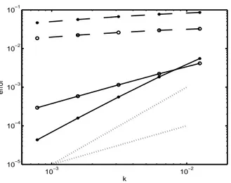
(67), hypotheses (A4) and (A4’) are satisfied. In Figure 1, we can see the results after integrating (30) till time T = 1 directly with (11) considering the last three terms of (30) as a source term. More precisely, we have considered in (11)
F = AhQh∂Ag(t) +BhQh∂Bg(t) +Phf(t), M1 = Ah,0,
M2 = Bh,0,
withh= 10−2. Moreover, we can also observe the results after applying formulas
(36)-(38) to avoid order reduction. In the first case, we can observe that the results are very poor while orders 2 and 1 are observed for the local and global errors respectively when applying the technique which is suggested in this paper. This corroborates Theorems 14 and 15 when h2 is negligible against k. Moreover, we see that, not only the order increases, but also the size of the errors considerably diminishes. We also notice that the same results are obtained with the suggested technique whenhdiminishes, so that no CFL condition is required.
Let us now consider, as a second experiment,
u0(x, y) =x(1−x)y(1−y) (71)
f(x, y, t) = e−t(−4x3+y+y2−2y3+x(−1 + 15y−3y2)−x2(−5 + 11y+y2)).
For such a problem the exact solution is u(x, y, t) = e−tx(1−x)y(1−y) which has homogeneous boundary values. Therefore, the only correction needed is due to the inhomogeneity f which is not zero on the boundary. In any case, (A4) and (A4’) are again satisfied.
10−3 10−2 10−5
10−4 10−3 10−2 10−1
k
error
Figure 1: Local error (*) and global error (o) without avoiding (discont.) and avoiding (cont.) order reduction when integrating problem (66) with Lie-Trotter method with non-commutable operators A and B given through (69) and data (70). Dotted lines represent the slope for orders 1 and 2.
10−3 10−2
10−5 10−4 10−3 10−2
k
error
10−3 10−2 10−6
10−5 10−4 10−3 10−2 10−1
k
error
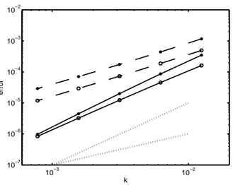
Figure 3: Local error (*) and global error (o) without avoiding (discont.) and avoid-ing (cont.) order reduction when integratavoid-ing problem (66) with Strang method with non-commutable operators A and B given through (69) and data (70). Dotted lines represent the slope for orders 1 and 2.
2. As the computational cost of the technique to avoid order reduction is negligible against the rest of the calculations of the method, the strategy which is suggested here is clearly better.
Let us now use Strang method for the same problem with data (70). As the opera-tors A and B do not commute, we have to use formulas (55)-(58). The order 2 of the local error which is given by Theorem 18 is clearly seen in Figure 3 and it seems that a summation-by-parts argument similar to that shown in [12] for vanishing boundary problems is also working here since the global error in fact behaves asO(k2) instead of
O(k), as assured by Theorem 21. Moreover, the difference between avoiding and not avoiding order reduction is seen to be even higher than with Lie-Trotter for the same problem.
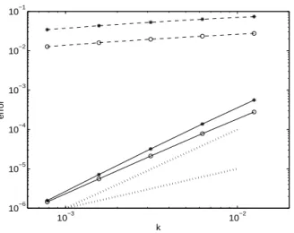
Let us now use Strang method for solving the same problem, but with data (71). When not avoiding order reduction, local and global orders are around 1.25, as stated in [12]. With the technique suggested here, we achieve order near 2 for both the local and global error, as in the example before. Figure 4 also shows that the size of the errors is much smaller with our technique at a very low additional cost. We would also like to remark that, using more complicated functionsa(x, y), b(x, y) in (66), we have numerically checked that order reduction is also avoided.
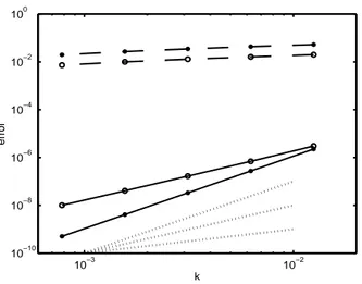
Finally, let us consider problem (66) with the laplacian operator. That is,
a(x, y) =b(x, y) = 1.
10−3 10−2 10−7
10−6 10−5 10−4 10−3 10−2
k
error
Figure 4: Local error (*) and global error (o) without avoiding (discont.) and avoid-ing (cont.) order reduction when integratavoid-ing problem (66) with Strang method with non-commutable operators A and B given through (69) and data (71). Dotted lines represent the slope for orders 1 and 2.
will use
u0(x, y) = (x2 −1/4)(y2−1/4), (72)
f(x, y, t) = e
−t
16(15−28y
2−
4x2(7 + 4y2)).
Now the exact solution of the problem isu(x, y) = (x2−1/4)(y2−1/4)e−t, which again satisfies regularity hypotheses (A4) and (A4’) although not vanishing at the boundary. With our technique, the local order is clearly 3 and the global one is 2, as stated by Theorems 17 and 19. However, as the solution does not vanish on the boundary, the results without avoiding order reduction are very poor. Figure 5 confirms that even in terms of the size of the errors.
Acknowledgements
This research has been supported by Ministerio de Ciencia e Innovaci´on project MTM2015-66837-P.