Modelos No Lineales Krolzig

Regime–Switching Models

HANS-MARTIN KROLZIG

Department of Economics and Nuffield College, University of Oxford.

[email protected] Hilary Term 2002

The course offers an introduction to regime-switching models, covering their theoretical prop-erties and the statistical tools for empirical research (including maximum likelihood estima-tion, model evaluaestima-tion, model selection and forecasting). With the Markov-switching vector autoregressive model, it presents a systematic and operational approach to the econometric modelling of time series subject to shifts in regime. The theory will be linked to empirical studies of the business cycle, using MSVAR for OX.

Course structure

(1) Introduction

(2) Types of regime-switching models (Assumptions, properties and estimation)

• Structural change and switching regression models

• Threshold models

• Smooth transition autoregressive models • Markov-switching vector autoregressions

(3) Assessing business cycles with regime-switching models (Markov-switching VECM of the UK labour market)

Basic literature

• Hamilton, J. D. (1989). A new approach to the economic analysis of nonstationary time series and the business cycle, Econometrica, 57, 357–384.

◦ Hamilton, J.D. (1994). Time Series Analysis. Princeton: Princeton University Press. Chapter 22.

• Hansen, B. (1999), Testing for Linearity, Journal of Economic Surveys, 13, 551–576. • Krolzig, H.-M., Marcellino, M. and G. E. Mizon, A Markov–Switching Vector

Equilib-rium Correction Model of the UK Labour Market, Empirical Economics, forthcoming. ◦ Potter, S. (1999), Nonlinear time series modelling: An introduction, Journal of

Eco-nomic Surveys, 13, 505–528.

• Ter¨asvirta, T. (1994). Specification, estimation, and evaluation of smooth transition autoregressive models, Journal of the American Statistical Association, 89, 208–218.

Monographies

◦ Franses, H.P. and D. van Dijk (2000). Nonlinear Time Series Models in Empirical

Fin-ance, Cambridge: Cambridge University Press.

◦ Granger, C.W.J. and T. Ter¨asvirta (1993). Modelling Nonlinear Economic

Relation-ships, Oxford, Oxford University Press.

◦ Kim, C.J. and C.R. Nelson (1999). State-Space Models with Regime Switching, Cam-bridge, MA: MIT Press.

◦ Krolzig, H.-M. (1997). ‘Markov-Switching Vector Autoregressions. Modelling, Statist-ical Inference and Application to Business Cycle Analysis’, Lecture Notes in Economics

1 Introduction

1.1 Linear time series models

Since Sims (1980) critique of traditional macroeconometric modeling, vector autoregressive (VAR) models are widely used in macroeconometrics. Their popularity is due to the flexib-ility of the VAR framework and the ease of producing macroeconomic models with useful descriptive characteristics, within statistical tests of economically meaningful hypothesis can be executed. Over the last two decades VARs have been applied to numerous macroeconomic data sets providing an adequate fit of the data and fruitful insight on the interrelations between economic data.

In the vector autoregressive model, theK-dimensional time series vectory_t= (y_1t, . . . , y_Kt)0

is generated by a vector autoregressive process of orderp

y_t=ν+A₁y_t−1+· · ·A_py_t−p+ε_t (1)

wheret= 1, . . . , T, theν is a vector of intercepts andA_i are coefficient matrices. The error process ε_t = (ε_1t, . . . , ε_Kt)0 is an unobservable, usually Gaussian, zero-mean white noise process,

ε_t∼WN(0,Σ).

that is, E[ε_t] = 0, E[ε_tε0_t] = Σ, and E[ε_tε0_s] = 0for s 6= t, where the variance-covariance matrixΣis time-invariant, positive-definite and non-singular.

The errors are such that the innovations can be interpreted as the one-step prediction errors of the system

ε_t=y_t−E[y_t|Y_t−1],

while the expectation ofy_tconditional on the information setY_t−1 = (y_t−1, y_t−2, . . . , y_1−p)

is given by the vector autoregression:

E[y_t|Y_t−1] =ν+

p

X

j=1

A_jy_t−j.

Although, in the past macroeconomic fluctuations and growth have been largely investigated using linear time series models, it is now increasingly recognized that the implications of the linear models

• linearity (invariance of dynamic multipliers with regard to the history of the system, size and sign of the shocks)

• time-invariance of parameters • Gaussianity

1.2 Regime-switching models

While the importance of regime shifts seems to be generally accepted, there is no established theory suggesting a unique approach for specifying econometric models that embed changes in regime. Increasingly, regime shifts are not considered as singular deterministic events, but the unobservable regime is assumed to be governed by an exogenous stochastic process. Thus regime shifts of the past are expected to occur in the future in a similar fashion.

When a time series is subject to regime shifts, the parameters of the statistical model will be varying. The basic idea of regime-switching models is that the process is time-invariant conditional on a regime variables_tindicating the regime prevailing at timet. Regime-switching models characterize a non-linear data generating process as piecewise linear by re-stricting the process to be linear in each regime, where the regime might be unobservable, and only a discrete number of regimes are feasible. The models within this class differ in their assumptions concerning the stochastic process generating the regime.

The primary objective of regime-switching models is to provide a systematic econometric ap-proach for the statistical analysis of multiple time series when the mechanism which generated the data is subject to regime shifts:

(i) extracting the information in the data about regime shifts in the past, (ii) estimating the parameters of the model consistently and efficiently, (iii) detecting recent regime shifts,

(iv) correcting the vector autoregressive model at times when the regime alters, (v.) incorporating the probability of future regime shifts into forecasts.

Regime-switching models studied represent a very general class which encompasses some alternative non-linear and time-varying models. In general, the model generate conditional heteroscedasticity and non-normality; prediction intervals are asymmetric and reflect the pre-vailing uncertainty about the regime.

1.2.1 Regime shifts

Characteristics

finite number — infinite number

deterministic — stochastic

single event — reoccurring within sample — reoccurring out of sample

observable — observable if DGP is known — unobservable even if DGP is known

(strongly) exogenous — endogenous

permanent — persistent — transitory

predictable — unpredictable

common — interrelated — independent

Granger causal — Granger noncausal

Implications

nonlinearity

time-varying parameters

1.2.2 The Conditional Process

The statistical model ofy_tdefined conditional upon the regimes_t∈ {1, . . . , M}. :

p(y_t|Y_t−1, X_t, s_t) =     

f(yt|Y_t−1, X_t, θ₁) ifs_t= 1

.. .

f(y_t|Y_t−1, X_t, θ_M) ifs_t=M.

wherep(y_t|Y_t−1, X_t, s_t)is the probability density function of the vector of endogenous vari-ables y_t = (y_1t, . . . , y_Kt)0 conditional upon the history of the process, Y_t−1 = {y_t−i}∞_i=1,

some (strongly) exogenous variablesX_t = {x_t−i}∞_i=0 and the regime variables_t.. θ_m is the parameter vector present in regimem.

It is usually assumed that the statistical model is linear in each regime, say s_t = m. In the following we focus on autoregressive processes

y_t=ν_m+α_m1y_t−1+. . .+α_mpy_t−p+ε_t, ε_t∼IID(0, σ2_m),

and their multivariate generalization: the vector autoregressive (VAR) process

y_t=ν_m+A_m1y_t−1+. . .+A_mpy_t−p+ε_t, ε_t∼IID(0,Σ_m).

1.2.3 The Regime Generating Process

If the stochastic process of y_t is defined conditionally upon the (unobservable) regime s_t, a complete description of the data generating mechanism requires the specification of the stochastic process which generates the regime:

Pr(s_t|Y_t−1, S_t−1, X_t;ρ)

2 Types of regime-switching models

2.1 Structural change and switching regression models

2.1.1 Structural break models

Structural break at timet=τ :

y_t= (

ν₁+Pp_i=1α_1iy_t−i+ε_t fort < τ

ν₂+Pp_i=1α_2iy_t−i+ε_t fort≥τ (2)

whereε_t∼IID(0, σ2).By using the indicator functionI(t;τ) :

I(t;τ) = (

1 fort > τ 0 fort≤τ.

the DGP can be rewritten as

y_t= ν₁+

p

X

i=1

α_1iy_t−i !

(1−I(t;τ)) + ν₂+

p

X

i=1

α_2iy_t−i !

I(t;γ) +ε_t.

Two different assumptions regarding the information structure

• τ is known: break is deterministic • τ is unknown: break is stochastic

2.1.2 Switching regression model

Closely related to the structural change model is the switching regression model, where the regime shifts are driven by an observable regime variables_t:

y_t= ν₁+

p

X

i=1

α_1iy_t−i !

(1−I(s_t= 1)) + ν₂+

p

X

i=1

α_2iy_t−i !

2.1.3 Maximum likelihood estimation under normality

Structural break at timet=τ :

y_t= (

ν₁+Pp_i=1α_1iy_t−i+ε_t fort < τ ν₂+Pp_i=1α_2iy_t−i+ε_t fort≥τ

whereε_t∼NID(0, σ2).

Two different assumptions regarding the information structure

• τ is known: break is deterministic

– Estimation: Split sample andOLSfor each regime;

– Test ofβ₁ =β₂ has standard asymptotics; whereβ_m = (ν_m, α₁, . . . , α_p). – The same technique can be used for switching regression models.

• τ is unknown: break is stochastic

– Grid search forτ ∈[0.15,0.85]T :

τ∗ = arg min

τ RSS(τ)

= arg min

τ τσˆ

2

1(τ) + (1−τ)ˆσ22(τ)

– Test ofβ₁ =β₂ has non-standard asymptotics asτ becomes nuisance variable. – See, inter alia, Andrews (1993), and Andrews and Ploberger (1994) and Banerjee,

2.2 Threshold models

2.2.1 The TAR model

In the threshold autoregressive model, the regime shifts are triggered by an observable, exo-genous transition variablex_tcrossing the thresholdc:

y_t= ν₁+

p

X

i=1

α_1iy_t−i !

(1−I(x_t;c)) + ν₂+

p

X

i=1

α_2iy_t−i !

I(x_t;c) +ε_t (4)

whereε_t∼IID(0, σ2).The indicator functionI(x_t;c)is of the type

I(x;c) =

(

1 ifg(x_t)> c 0 ifg(x_t)≤c.

Forx_t=ta model with a structural break at timet=coccurs

2.2.2 The SETAR model

If the transition variable is a lagged endogenous variable y_t−d with delay d > 0, the self-exciting threshold autoregressive model results:

y_t= ν₁+

p

X

i=1

α_1iy_t−i !

(1−I(y_t−d;c)) + ν₂+

p

X

i=1

α_2iy_t−i !

I(y_t−d;c) +ε_t (5)

whereε_t∼IID(0, σ2). . cis again the threshold. Note that the model can be written as:

y_t=ν(s_t) +

p

X

i=1

α_i(s_t)y_t−i+ε_t

where for a given but unknown threshold c, the ‘probability’ of the unobservable regime, say

s_t= 2is given by

Pr (s_t= 1|S_t−1, Y_t−1) =I(y_t−d;c) = (

1 if g(y_t−d)> c 0 if g(y_t−d)≤c.

Thus in the self-exciting threshold autoregressive (SETAR) model, the regime-generating pro-cess is not assumed to be exogenous but directly linked to the lagged endogenous variable

SETAR Models of US GNP of Tiao and Tsay (1994) and Potter (1993)

Quarterly growth rate of U.S. GNP,∆y_t:

∆y_t=µ(s_t) +X5

i=1

α_i(s_t)∆y_t−i+u_t, u_t∼IID(0, σ2(s_t))

2-regime SETAR withd= 2.

Empirical models:

• Thresholdr≈0:s_t= (

1 if∆y_t−2 > r 2 if∆y_t−2 ≤r

• Moving swiftly out of recessions: α(₂L) <<0

2.2.3 Maximum likelihood estimation under normality

(i) For given delayd,and thresholdc:

• Sample split according toI(y_t−d;c). • OLSregression for each regime separately:

ˆ

β_m = (X0_mX_m)−1X0_my_m

ˆem =

I−Xm(X0mXm)−1X0m

ym

ˆ

σ_m2 = T_m−1ˆe0_mˆe_m

whereX_mandy_mcollect the observations from regimem,i.e. those observations at timetwiths_t=m. T_mis the number of observations in regimem.

• Alternative indicator functions can be used in a single regression, constraining the residual error variance to be constant across regimes (see, for example, Potter, 1993, p.113.).

(ii) Grid search overdand c: select the pair (c, d) that minimizes the overall residual sum of squares (RSS)

(c, d)∗= arg min

(c,d)RSS(c, d) = arg min(c,d) M

X

m=1

T_mσˆ2_m

Usually the search overc(givend)is restricted such that

minT_m ≥0.15T.

(iii) Whenpis unknown, fit is usually traded against parsimony. A search is made over all values ofp ≤ pmax, and the preferred order is often taken to be that which minimizes

AIC.

p∗ = arg min

p

(

AIC(p) = XM

m=1

T_mln ˆσ_m2 + 2 (p+ 1) )

.

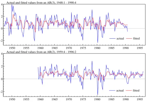
1950 1955 1960 1965 1970 1975 1980 1985 1990 1995 -2

0 2

4 Actual and fitted values from an AR(3), 1948:1 - 1990:4

actual fitted

1950 1955 1960 1965 1970 1975 1980 1985 1990 1995 -2

0 2

4 Actual and fitted values from an AR(2), 1959:4 - 1996:2

actual fitted

Figure 1 Linear AR model of US GNP growth.

1950 1955 1960 1965 1970 1975 1980 1985 1990 1995 -2

0 2

4 Actual and fitted values from a SETAR(2;2,2), 1947:4 - 1990:4

actual fitted

1950 1955 1960 1965 1970 1975 1980 1985 1990 1995 -2

0 2

4 Actual and fitted values from SETAR(2;2,2), 1959:4 - 1996:2

actual fitted

2.3 Smooth transition autoregressive models

2.3.1 The STAR model

In the smooth transition autoregressive model popularized by Granger and Ter¨asvirta (1993), the weight attached to the regimes depends on the realization of exogenous or lagged endo-genous variablesz_t:

Pr(s_t= 2|S_t−1, Y_t−1, X_t) =G(z_t;γ, c),

where the transition functionG(z_t;γ, c)is a continuous function determining the weight of regime 2, and usually bounded between 0 and 1.

The STAR model is closely associated with the work of Ter¨asvirta (1994), (1998)

y_t= ν₁+

p

X

i=1

α_1iy_t−i !

(1−G(z_t;γ, c)) + ν₂+

p

X

i=1

α_2iy_t−i !

G(z_t;γ, c) +ε_t (6)

whereε_t∼IID(0, σ2).

The transition variable z_t can be a lagged endogenous variable (z_t = y_t−d for d > 0),

an exogenous variable (z_t = x_t), or a function of some lagged endogenous and exogenous variables: z_t = g(y_t−d, x_t).Forz_t = ta model with smoothly changing parameters results (see Lin and Ter¨asvirta, 1994). cis the threshold,γ is the smoothness parameter.

The STAR model (6) exhibits two regimes

• associated with the extreme values of the transition function: G(z_t;γ, c) = 1 and

G(z_t;γ, c) = 0;

• transition from one regime to the other is gradual;

• the regime occurring at timetis observable (for givenz_t;γ, c) and can be determined byG(z_t;γ, c).

For multiple-regime STAR models: see Dijk (1999).

Choices for the transition functionG(z_t;γ, c) :

• logistic cumulative density function (LSTAR): different behavior for positive versus negative values ofz_trelatively toc

G(z_t;γ, c) = 1

1 + exp{−γ(z_t−c)}.

Forγ → ∞:LSTAR→SETAR:

G(z_t;γ, c) =I(z_t> c);

Forγ →0 :LSTAR→linear AR

• exponential function (ESTAR): different behavior for small versus large deviations ofz_t

from the thresholdc:

G(z_t;γ, c) = 1−exp−γ(z_t−c)2 .

Forγ → ∞andγ →0 :ESTAR→linear AR:

G(z_t;γ, c) = 0.

• quadratic logistic function:

G(z_t;γ, c) = 1

1 + exp{−γ(z_t−c₁)(z_t−c₂)}.

Forγ → ∞:quadratic LSTAR→3-regime SETAR:

G(z_t;γ, c) = 1−I(c₁ < z_t< c₂);

Forγ →0 :quadratic LSTAR→linear AR

G(z_t;γ, c) = 0.5.

Properties of STAR models

• Little is known about the conditions under which STAR models are stationary; • Stationarity has to be evaluated by numerical procedures;

• Even under stationarity: Rich variability of the implied dynamics – unique equilibrium

– multiple equilibria – limit cycles

– strange attractors (chaos)

STAR models of US Industrial Production

Ter¨asvirta and Anderson (1992): 2-regime LSTAR model of the annual growth rate of US Industrial Production (quarterly data from 1961-1986):

∆₄y_t= ν₁+

9

X

i=1

α_1i∆₄y_t−i !

(1−G(·)) + ν₂+

9

X

i=1

α_2i∆₄y_t−i !

G(·) +ε_t

with the transition function

G(y_t−3;γ, c) = 1

1 + exp{−45(∆y_t−3−0.0061)/σ_y}.

Properties of business cycle

• expansion: ∆y_t−3 >0.61%

largest root ofα₁(L): modulus= 0.76and period= 61quarters • contraction:∆y_t−3 <0.61%

largest root ofα₂(L): modulus= 1.1and period= 8.9quarters

Multivariate Smooth Transition Models

y_t= ν₁+

p

X

i=1

A_1iy_t−i !

(1−G(z_t;γ, c)) + ν₂+

p

X

i=1

A_2iy_t−i !

G(z_t;γ, c) +ε_t

wherey_t= (y_1t,· · ·, y_Kt)0, ε_t∼IID(0,Σ), A_miis a(K×K)matrix,ν_mis(K×1). Tsay (1998) describes a specification procedure for multivariate threshold models.

Suppose now that y_t isI(1),but a linear combination e_t = β0y_tis stationary with mean µ.

Then a smooth transition equilibrium correction model is of interest:

Asymmetric VECMs

∆y_t=α₁(1−G(e_t−1;γ, µ)) (e_t−1−µ) +α₂G(e_t−1;γ, µ) (e_t−1−µ) +ε_t.

LSTAR: positive versus negative deviations from equilibrium

G(e_t−1;γ, µ) = 1

1 + exp{−γ(e_t−1−µ)}.

SETAR results forγ → ∞

G(e_t−1;γ, µ) =I(e_t−1 > µ)

ESTAR: small versus large deviations from equilibrium

G(e_t−1;γ, µ) = 1−exp−γ(e_t−1−µ)2 .

Interesting case: random walk behavior in regime 1 (β0α₁ = 0) and mean adjustment in regime 2 (β0α₂ <0)

2.3.2 Maximum likelihood estimation

STAR model

y_t = x0_tβ₁(1−G(z_t;γ, c)) +x0_tβ₂G(z_t;γ, c) +ε_t, ε_t∼IID(0, σ2)

Non-linear least squares (NLS) estimation ofθ= (β₁0, β₂0;γ, c)0 :

ˆ

θ= arg min

θ RSS= arg minθ T

X

t=1

ε2_t(θ)

whereε_t(θ) =y_t−[x0_tβ₁(1−G(z_t;γ, c)) +x0_tβ₂G(z_t;γ, c)].

• Under the assumption of normality,ε_t∼NID(0, σ2) :NLS=ML.

• Estimation via numerical optimization procedure (see e.g. Hendry, 1995, Appendix A5).

– local maxima! – convergence?

• Starting values:

– Conditional uponγ andc:OLSestimation ofβ= (β₁00, β₂0)0

ˆ

β(γ, c) =

T

X

t=1

x_t(γ, c)x_t(γ, c)0−1x_t(γ, c)y_t

wherex_t(γ, c) = (x0_t(1−G(z_t;γ, c)), x0_tG(z_t;γ, c))0;

– Grid search overγandc: minRSS(γ, c).

• Concentrating the likelihood (RSS) function:

– Conditional uponγ andc:OLSestimation ofβ= (β₁00, β₂0)0; – NLS ofγandc: minRSS(γ, c).

• Problem: precise estimation ofγ

– reason: for large values ofγ,the shape of the logistic function changes only little – accurate estimate ofγrequires many observations in the immediate neighbourhood

of the thresholdc.

2.3.3 Model selection

An empirical specification procedure

Ter¨asvirta (1994) based on the Granger and Ter¨asvirta (1993) recommendation of a specific-to-general procedure for non-linear models.

(1) Specify appropriate linear AR(p) model;

(2) Test the null hypothesis of linearity against the STAR alternative; (3) If linearity is rejected, selectz_tand specifyG(z_t;γ, c);

(4) Estimate the STAR model;

(5) Evaluate the STAR model using diagnostic tests; (6) If misspecification is detected, modify the model; (7) Use the model for descriptive or forecasting purposes.

Testing for STAR nonlinearity

Problem: Under the null of linearity, some ‘nuisance’ parameters are not identified

null hypothesis nuisance parameters

(ν₁, α₁₁, . . . α_1p) = (ν₂, α₂₁, . . . α_2p) γ; c

γ = 0 (ν₁, α₁₁, . . . α_1p)−(ν₁, α₁₁, . . . α_1p); c

→ conventional statistical theory can not be applied (see Davies, 1977, Davies, 1987 and Hansen, 1996b)

→non-standard distributions

→critical values have to be determined by means of simulation methods.

Solution proposed by Luukkonen, Saikkonen and Ter¨asvirta (1988):

Replace the transition functionG(z_t;γ, c)by a suitable Taylor approximation. In the reparametrized model, the identification problem is no longer present. Linearity can be tested by means of a Lagrange multiplier (LM) statistic, which has a standard asymptoticχ2−distribution under the null.

→Test against LSTAR: Luukkonen et al. (1988). →Test against LSTAR: Granger and Ter¨asvirta (1993).

Diagnostic checking in STAR models

Eitrheim and Ter¨asvirta (1996) discuss formal diagnostic tests for STAR models

• Jarque-Bera test for normality of the residuals • LM type test for serial autocorrelation

• LM test for remaining nonlinearity (two-regime STAR against the alternative of an ad-ditive STAR model)

Hans–Martin Krolzig Hilary Term 2002

Regime–Switching Models

2.4 Markov-switching vector autoregressions

2.4.1 The MS-VAR model

In Markov-switching vector autoregressive (MS-VAR) models it is assumed that the regimes_t

is generated by a hidden discrete-state homogeneous and ergodic Markov chain:

Pr(st|S_t−1, Y_t−1, X_t) = Pr(st|s_t−1;ρ)

defined by the transition probabilities

p_ij = Pr(s_t+1=j|s_t=i).

The conditional process is a VAR(p) with

• shift in the mean (MSM-VAR): once-and-for-all jump in the time series

y_t−µ(s_t) =A₁(s_t) (y_t−1−µ(s_t−1)) +. . .+A_p(s_t) (y_t−p−µ(s_t−p)) +u_t,

• shift in the intercept (MSI-VAR): smooth adjustment of the time series

y_t=ν(s_t) +A₁(s_t)y_t−1+. . .+A_p(s_t)y_t−p+u_t,

A major advantage of the MS-VAR is its flexibility, see Krolzig (1997).

Special MS-VAR Models

MSM MSI Specification

µvarying µinvariant νvarying νinvariant

A_j Σinvariant MSM–VAR linear MVAR MSI–VAR linear VAR

invariantΣvarying MSMH–VAR MSH–MVAR MSIH–VAR MSH–VAR

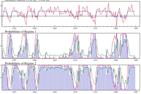
1955 1960 1965 1970 1975 1980 1985 0

2.5

MSM(2)-AR(4), 1952 (2) - 1984 (4)

1955 1960 1965 1970 1975 1980 1985 .5

1 Probabilities of Regime 1

1955 1960 1965 1970 1975 1980 1985 .5

1 Probabilities of Regime 2

Figure 3 Hamilton’s MSM(2)-AR(4) model.

Markov-switching autoregressive models of US GNP

Hamilton (1989): 2-regime MS-AR model for the quarterly growth rate of U.S. GNP:

∆y_t−µ(s_t) =X4

k=1

α_k(∆y_t−k−µ(s_t−k)) +u_t, u_t|s_t∼NID(0, σ2)

Two regimes “state of the business cycle”

µ(s_t) = (

µ₁ >0 ifs_t= 1(‘expansion’)

µ₂ <0 ifs_t= 2(‘contraction’)

generated by an ergodic Markov chain

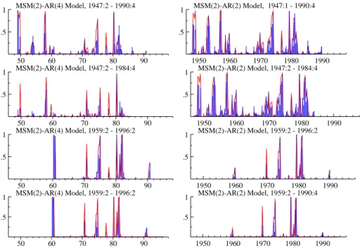
50 60 70 80 90 .5

1 MSM(2)-AR(4) Model, 1959:2 - 1996:2 50 60 70 80 90 .5

1 MSM(2)-AR(4) Model, 1959:2 - 1996:2 50 60 70 80 90 .5

1 MSM(2)-AR(4) Model, 1947:2 - 1990:4

50 60 70 80 90 .5

1 MSM(2)-AR(4) Model, 1947:2 - 1984:4

1950 1960 1970 1980 1990 .5

1 MSM(2)-AR(2) Model, 1959:2 - 1996:2 1950 1960 1970 1980 1990 .5

1 MSM(2)-AR(2) Model, 1947:1 - 1990:4

1950 1960 1970 1980 1990 .5

1 MSM(2)-AR(2) Model, 1959:2 - 1990:4 1950 1960 1970 1980 1990 .5

1 MSM(2)-AR(2) Model, 1947:2 - 1984:4

Figure 4 MSM(2)-AR models of US GNP growth.

50 60 70 80 90 .5

1‘High’ Growth Regime, H

1948:2-1990:4

50 60 70 80 90 .5

1

1948:2-1984:4

50 60 70 80 90 .5

1‘Recession’ Regime, L

50 60 70 80 90 .5

1

50 60 70 80 90 .5

1

1960:2-1990:4

50 60 70 80 90 .5

1

50 60 70 80 90 .5

1

1960:2-1996:2

50 60 70 80 90 .5

1

2.4.2 State-Space Representation

The framework for the statistical analysis of MS-VAR models is the state-space form. The advantage of viewing MS-VAR models in this way is that general concepts as the likelihood principle and a recursive filter algorithm can be introduced. The state-space model consists of the set of measurement and transition equations.

Measurement or observation equation (conditional process): The measurement equation describes the relation between the unobserved state vector ξ_t and the observed time series vectory_t. Here, the predetermined variablesY_t−1and the vector of Gaussian disturbances u_t

enter the model.

Example: MSI(M)-VAR(1) model

y_t = Mξ_t+A₁y_t−1+u_t

whereM=

h

ν₁ · · · ν_M i

andξ_t=   

I(s_t= 1)

.. .

I(s_t=M)

 

 withI(s_t=m) =

(

1 ifs_t=m

0 otherwise

State or transition equation (regime generating process): The state vector ξ_t follows a Markov chain subject to a discrete adding-up restriction. The Markov chain governing the state vectorξ_tcan be represented as a first-order vector autoregression (cf. Hamilton, 1994b):

ξ_t+1 =Fξ_t+v_t+1, v_t+1 ≡ξ_t+1−E[ξ_t+1|{ξ_t−j}∞_j=0]

MSM-VAR processes as linearly transformed VAR processes

MSM(M)–VAR(p) Process,p≥0

A(L) (y_t−µ(s_t)) =u_t ⇐⇒     

y_t = µ(s_t) +z_t µ_t = Mξ_t,

A(L)z_t = u_t, u_ti.i.d. WN(0,Σ_u).

State Space Representation

y_t−µ_y = Mζ_t+Jz_t ζ_t = Fζ_t−1+v_t

zt = Azt−1+ut

⇐⇒           

y_t−µ_y = h

M J

i " _ζ

t zt # " ζ_t zt # = " F 0 0 A # " ζ_t−1

zt−1

# + " v_t ut #

ζ_t =   

ξ_1,t

.. .

ξ_M−1,t   −    ¯ ξ₁ .. . ¯ ξ_M−1

   F =   

p_1,1−p_M,1 . . . p_M−1,1−p_M,1

..

. ...

p_1,M−1−p_M,M−1 . . . p_M−1,M−1−p_M,M−1   ,

M = h µ₁−µ_M . . . µ_M−1−µ_M i

,

zt =

      z_t z_t−1

.. .

z_t−p+1     

, A=      

A₁ . . . A_p−1 A_p

IK 0 0

. .. .._. .._.

0 . . . I_K 0     

, ut=       u_t 0 .. . 0      ,

J = e0₁⊗I_K.

A VARMA-Representation Theorem

MSM(M)−VAR(p)

y_t = µ_y+Mζ_t+z_t

z_t = A(L)−1u_t, A(L) =I_K−A₁L−. . .−A_pLp ζ_t = F(L)−1v_t, F(L) =I_M−1− FL

Moving-average representation:

y_t=µ_y+MF(L)−1v_t+A(L)−1u_t

Final-equations-form VARMA(M+Kp−1,M+Kp−2):

2.4.3 Related models

Mixture of normals

The mixture of normals model is characterized by serially independently distributed regimes:

Pr(s_t|S_t−1, Y_t−1) = Pr(s_t;ρ).

This is a special case of the MS-AR model, which results when the transition probabilities are independent of the history of the regime.

The conditional probability distribution ofy_tis independent ofS_t−1,

p(y_t|Y_t−1, S_t−1) =p(y_t|Y_t−1),

and the regimes are Granger non-causal fory_t. Even so, this model can be considered as a restricted MS-VAR model where the transition matrix has rank one. Moreover, if only level of the time series is regime-dependent, the model is observationally equivalent to time-invariant linear processes with non-normal errors.

Time-varying transition probabilities (endogenous switching)

All the previously mentioned models are special cases of an endogenous selection model: The transition probabilities p_ij are not time-invariant parameters, but functions of the observed time series vectory_t−dor some exogenous variablesx_t:

Pr(s_t= 1|S_t−1, Y_t−1, X_t) =F(z_t, s_t−1;γ, c) = (

1−F₁₂(z_t;γ, c) if s_t−1 = 1 F₂₁(z_t;γ, c) if s_t−1 = 2.

For example, in the case of an exponential function the time-varying transition probabilities are given by:

p_ijt=F_ij(z_t;γ, c) = 1−exp−γ_ij(z_t−c_ij)2 fori6=j

andp_iit = 1−PM_j=1p_ijt.

In contrast to an MS-AR model, the regime switching rule also depends on the history of the observed variables. Since the observed variables contain additional information on the conditional probability distribution of the states, the regime generating process is no longer Markovian:

Pr(st|S_t−1, Y_t−1)a.e.6= Pr(st|s_t−1).

−5 −4 −3 −2 −1 0 1 2 3 4 5 0.2

0.4

Regime−dependent densities

p(y

t|st=1,Yt−1)

p(y

t|st=2,Yt−1)

−5 −4 −3 −2 −1 0 1 2 3 4 5

0.1 0.2

0.3 Density of yt given Yt−1

p(y_t|Y_t−1) for Pr(s_t=1|Y_t−1)=.3 p(y_t|Y_t−1) for Pr(s_t=1|Y_t−1)=.5

−5 −4 −3 −2 −1 0 1 2 3 4 5

0.0 0.5

1.0 Regime inference after observation of yt

Pr(s_t=1|Y_t) for Pr(s_t=1|Y_t−1)=.3 Pr(s_t=1|Y_t) for Pr(s_t=1|Y_t−1)=.5

Figure 6 Regime inference.

2.4.4 Regime inference

The discrete support of the state in the MS-AR model allows to derive the complete conditional distribution of the unobservable state variable

• instead of deriving the first two moments, as in the Kalman filter (cf. Kalman, 1960, Kalman and Bucy, 1961, and Kalman, 1963) for Gaussian linear state-space models, • the grid-approximation suggested by Kitagawa (1987) for non-linear, non-normal

state-space models.

Literature

• The filtering and smoothing algorithms for time series models with Markov-switching regimes are closely related to Hamilton (1988, 1989, 1994a) building upon ideas of Cosslett and Lee (1985).

• The basic filtering and smoothing recursions had been introduced by Baum, Petrie, Soules and Weiss (1970) for the reconstruction of hidden Markov chains.

• Lindgren (1978) applied their algorithms to regression models with Markovian regime switches.

Filtering

The filter introduced by Hamilton (1989) can be described as an iterative algorithm for calcu-lating the optimal inference ofξ_t+1 on the basis of the information set intconsisting of the observed values ofy_t, namelyY_t= (y_t0, y_t0₋₁, . . . , y0_1−p)0. It might also be viewed as a discrete version of the Kalman filter for the state-space model

y_t = X_tBξ_t+u_t, ξ_t+1 = Fξ_t+v_t+1.

For given parameters, the discrete-state algorithm under consideration summarizes the condi-tional probability distribution of the state vectorξ_tby

ˆ

ξ_t|t=E[ξ_t|Y_t] =   

Pr(ξ_t=ι₁|Y_t)

.. .

Pr(ξ_t=ι_N|Y_t)   .

Since each component ofξˆ_t|tis a binary variable,ξˆ_t|tpossesses not only the interpretation as the conditional mean, which is the optimal inference of ξ_t givenY_t, but it also presents the probability distribution ofξ_tconditional onY_t.

The filtering algorithm computes ξˆ_t|t by deriving the joint probability density of ξ_t and y_t

conditioned on observationsY_t.

By invoking the law of Bayes, the posterior probabilitiesPr(ξt|y_t, Y_t−1)are given by

Pr(ξt|Y_t)≡Pr(ξt|y_t, Y_t−1) = p(yt|ξt, Yt−1)Pr(ξt|Yt−1)

p(y_t|Y_t−1) ,

with the prior probability

Pr(ξ_t|Y_t−1) =X

ξt−1

Pr(ξ_t|ξ_t−1)Pr(ξ_t−1|Y_t−1)

and the density

p(yt|Y_t−1) =X

ξt

p(y_t, ξt|Y_t−1) =X

ξt

Pr(ξt|Y_t−1)p(yt|ξ_t, Y_t−1).

Note that the summation involves all possible values ofξ_tandξ_t−1. Letη_tbe the vector of the densities ofy_tconditional onξ_tandY_t−1

η_t=   

p(y_t|θ₁, Y_t−1)

.. . p(y_t|θ_N, Y_t−1)

  =   

p(y_t|ξ_t=ι₁, Y_t−1)

.. .

p(y_t|ξ_t=ι_N, Y_t−1)   ,

Then, the contemporaneous inferenceξˆ_t|tis given in matrix notation by

ˆ

ξ_t|t = ηt ˆ ξ_t|t−1

10

N(ηtξˆt|t−1)

, (7)

where denotes the element-wise matrix multiplication and 1_N = (1, . . . ,1)0 is a vector consisting of ones. The filter weights for each regime the conditional density of the observation

y_t, given the vectorθ_mof AR parameters of regimem, with the predicted probability of being in regime m at time t given the information set Y_t−1. Thus, the instruction (7) describes the filtered regime probabilities ξ_t|t as an update of the estimate ξ_t|t−1 ofξ_t given the new informationy_t.

The transition equation implies that the vectorξˆ_t+1|tof predicted probabilities is a linear func-tion of the filtered probabilitiesξˆ_t|t:

ˆ

ξ_t+1|t= Fξˆ_t|t. (8)

The sequence{ξˆ_t|t−1}T_t=1can therefore be generated by iterating on (7) and (8), which can be summarized as:

ˆ

ξ_t+1|t = F(ηt ˆ ξ_t|t−1)

10_(η

tξˆt|t−1)

. (9)

In the prevailing Bayesian context, ξˆ_t|t−1 is the prior distribution ofξ_t. The posterior distri-butionξˆ_t|tis calculated by linking the new informationy_twith the prior via Bayes’ law. The posterior distributionξˆ_t|tbecomes the prior distribution for the next stateξ_t+1and so on.

Smoothing

The filter recursions deliver estimates forξ_t, t = 1, . . . , T based on information up to time point t. This is a limited information technique, as we have observations up tot=T. In the following, full-sample information is used to make an inference about the unobserved regimes by incorporating the previously neglected sample informationY_t+1.T = (y0_t+1, . . . , y0_T)0 into the inference aboutξ_t. Thus, the smoothing algorithm gives the best estimate of the unobserv-able state at any point within the sample.

The smoothing algorithm proposed by Kim (1994) may be interpreted as a backward filter that starts at the end pointt=T of the previously applied filter.

The full–sample smoothed inferences ξˆ_t|T can be found by iterating backward fromt=T − 1,· · ·,1by starting from the last output of the filterξˆ_T|T and by using the identity

Pr(ξ_t|Y_T) = X

ξt+1

Pr(ξ_t, ξ_t+1|Y_T)

= X

ξt+1

For pure AR models with Markovian parameter shifts, the probability laws for y_t and ξ_t+1

depend only on the current stateξ_tand not on the former history of states. Thus, we have

Pr(ξt|ξ_t+1, Y_T) ≡ Pr(ξt|ξ_t+1, Y_t, Y_t+1.T)

= p(Yt+1.T|ξt, ξt+1, Yt)Pr(ξt|ξt+1, Yt)

p(Y_t+1.T|ξ_t+1, Y_t) = Pr(ξ_t|ξ_t+1, Y_t).

It is therefore possible to calculate the smoothed probabilitiesξˆ_t|T by getting the last term from the previous iteration of the smoothing algorithm ξˆ_t+1|T, while it can be shown that the first term can be derived from the filtered probabilities ξˆ_t|t,

Pr(ξ_t|ξ_t+1, Y_t) = Pr(ξt+1|ξt, Yt)Pr(ξt|Yt) Pr(ξ_t+1|Y_t)

= Pr(ξt+1|ξt)Pr(ξt|Yt)

Pr(ξ_t+1|Y_t) . (11)

If there is no deviation between the full information estimate,ξˆ_t+1|T, and the inference based on the partial information, ξˆ_t+1|t, then there is no incentive to update ξˆ_t|T = ˆξ_t|t and the filtering solutionξˆ_t|tcannot be further improved.

In matrix notation, (10) and (11) can be condensed to

ˆ ξ_t|T =

F0_(ˆξ

t+1|T ξˆt+1|t)

ξˆ_t|t, (12)

2.4.5 Maximum Likelihood estimation

The Likelihood Function

In econometrics the so-called Markov model of switching regressions considered by Goldfeld and Quandt (1973)

y_t=x0_tβ_m+u_mt, u_mt∼NID(0, σ2_m)form= 1,2

has been one of the first attempts to analyze regressions with Markovian regime shifts. Gold-feld and Quandt (1973) claimed to derive maximum likelihood estimates by maximizing their “likelihood” function, which would be in terms of our model

Q(θ, ρ, ξ₀) =YT

t=1

η_t(θ)0ξ_t|0(ρ, ξ₀),

whereη_tis again an(M×1)vector collecting the conditional densitiesp(yt|Y_t−1, θ_m), m= 1, . . . , M, andξ_t|0= Ftξ₀are the unconditional regime probabilities.

Unfortunately, the functionQ(θ, ρ, ξ₀)isnotthe likelihood function as pointed out by Cosslett and Lee (1985).

Derivation of the likelihood function as a by–product of the filter:

L(λ|Y) := p(Y_T|Y₀;λ)

= YT

t=1

p(Y_t|Y_t−1, λ)

= T Y t=1 X ξt

p(yt|ξ_t, Y_t−1, θ) Pr(ξt|Y_t−1, λ)

= YT

t=1

η0_tξˆ_t|t−1

= YT

t=1

η0_tFξˆ_t−1|t−1.

The conditional densitiesp(y_t|ξ_t−1 =ι_i, Y_t−1)are mixtures of normals. Thus, the likelihood function is non-normal:

L(λ|Y) =

T Y t=1 N X i=1 N X j=1

p_ij Pr(ξ_t−1 =ι_i|Y_t−1, λ)p(y_t|ξ_t=ι_j, Y_t−1, θ)

= YT

t=1 N X i=1 N X j=1

p_ij ξˆ_{i.t−1|t−1}

(2π)−K/2_|Σ

j|−1/2exp

−1₂u0_jtΣ−_j1u_jt

,

where u_jt = y_t−E[y_t|ξ_t = ι_j, Y_t−1]and N = Mp+1 in MSM specifications orN = M

Normal Equations of theMLEstimator

The maximum likelihood (ML) estimates can be derived by maximization of likelihood func-tionL(λ|Y)subject to the adding-up restrictions:

P1M = 1

10_Mξ₀ = 1

and the non-negativity restrictions

ρ≥0, σ≥0, ξ₀≥0.

If the non-negativity can be ensured, theMLestimateλ˜ is given by the first-order conditions (FOCs) of the constrained log-likelihood function

lnL∗(λ) := lnL(λ|Y_T)−κ0₁(P1_M −1_M)−κ₂(10_Mξ₀−1). (13)

Then the FOCs are given by the set of simultaneous equations

∂lnL(λ|Y)

∂θ0 = 0

∂lnL(λ|Y) ∂ρ0 −κ

0

1(10M ⊗IM) = 0

∂lnL(λ|Y) ∂ξ₀0 −κ21

0

M = 0,

where it is assumed that the interior solution of these conditions exits and is well-behaved, such that the non-negativity restrictions are not binding.

The derivation of the log-likelihood function concerning the parameter vector θleads to the score function

∂lnL(λ|Y)

∂θ0 =

1

L

Z

∂p(Y|ξ, θ)

∂θ0 Pr(ξ|ξ0, ρ)dξ = 1

L

Z

∂lnp(Y|ξ, θ)

∂θ0 p(Y|ξ, θ)Pr(ξ|ξ0, ρ)dξ =

Z

∂lnp(Y|ξ, λ)

∂θ0 Pr(ξ|Y, λ)dξ

= XT

t=1

X

ξt

∂lnp(y_t|ξ_t, Y_t−1, λ)

∂θ0 Pr(ξt|YT, λ)

Maximization of the constrained likelihood function with respect to the parameter vectorρof the hidden Markov chain leads to

∂lnL(λ|Y)

∂ρ0 =

1

L

Z

p(Y|ξ, θ)∂Pr(ξ|ξ0, ρ) ∂ρ0 dξ

= 1

L

Z

∂ln Pr(ξ|ξ₀, ρ)

∂ρ0 p(Y|ξ, θ)Pr(ξ|ξ0, ρ)dξ =

Z

∂ln Pr(ξ|ξ₀, ρ)

Thus, the MLestimator of the vector of transition probabilities ρ is equal to the transition probabilities in the sample calculated with the smoothed regime probabilities:

˜ p_ij =

P_T

t=1_PPr(st=j, st−1 =i|YT;λ) T

t=1Pr(st−1=i|YT;λ)

.

The EM Algorithm

As shown in Hamilton (1990), the Expectation-Maximization (EM) algorithm introduced by Dempster, Laird and Rubin (1977) can be used in conjunction with the filter to obtain the maximum likelihood estimates of the model’s parameters.

The EM algorithm is an iterative ML estimation technique designed for a general class of models where the observed time series depends on some unobservable stochastic variables. For the hidden Markov-chain model an early precursor to the EM algorithm was provided by Baum et al. (1970) building upon ideas in Baum and Eagon (1967). The consistency and asymptotic normality of the proposed MLestimator were studied in Baum and Petrie (1966) and Petrie (1969). Their work has been extended by Lindgren (1978) to the case of regression models with Markov-switching regimes.

Each iteration of the EM algorithm consists of two steps:

• In the expectation step (E), the unobserved states ξ_t are estimated by their smoothed probabilitiesξˆ_t|T. The conditional probabilitiesPr(ξ|Y, λ(j−1))are calculated with the filter and smoother by using the estimated parameter vectorλ(j−1)of the last maximiz-ation step instead of the unknown true parameter vectorλ.

• In the maximization step (M), an estimate ofλis derived as a solutionλ˜of the FOCs of

MLestimation, where the conditional regime probabilitiesPr(ξ_t|Y, λ) are replaced by the smoothed probabilitiesξˆ_t|T(λ(j−1)_{)of the last expectation step. Thus, the dominant} source of non-linearities in the FOCs is eliminated. If the score, i.e. the gradient of

lnL(λ|Y_T), would have been linear inξ, this procedure were equivalent to replacing the unobserved latent variablesξin the FOCs with their expectationξˆ_t|T.

Equipped with the new parameter vectorλthe filtered and smoothed probabilities are updated and so on. Thus, each EM iteration involves a pass through the filter and smoother, followed by an update of the first order conditions and the parameter estimates and is guaranteed to increase the value of the likelihood function.

Determination of the number of regimes in MS-VAR models

Testing for the number of regimes in an MS-VAR model is a difficult enterprise:

Conventional testing approaches are not applicable due to the presence of unidentified nuis-ance parameters under the null of linearity.

null hypothesis nuisance parameters

µ₁=µ₂ p₁₂, p₂₁ p₁₂= 0(s₀ = 1) µ₂

The presence of the nuisance parameters gives the likelihood surface sufficient freedom so that one cannot reject the possibility that the apparently significant parameters could simply be due to sampling variation. The scores associated with parameters of interest under the alternative may be identically zero under the null.

Davies (1977, 1987) derived an upper bound for the significance level of the likelihood ratio test statistic under nuisance parameters.

Formal tests of the Markov-switching model against linear alternative employing standardized likelihood ratio test designed to deliver (asymptotically) valid inference have been proposed by Hansen (1992, 1996a), Garcia (1998), but they are computationally demanding.

The results of Ang and Bekaert (1998) indicate that critical values of theχ2(r+n)distribution can be used approximately whereris the number of restricted parameters andnis the number of nuisance parameters.

Alternatives

• Information criteria:

AIC = −2 logL/T + 2n/T,

SC = −2 logL/T +nlog(T)/T,

HQ = −2 logL/T + 2nlog(log(T))/T,

whereLis the maximized likelihood,nis the number of parameters andT is the sample size: see Akaike (1985), Schwarz (1978), and Hannan and Quinn (1979).

Hans–Martin Krolzig Hilary Term 2002

Regime–Switching Models

3 Prediction and structural analysis with regime-switching models

Forecasting and structural analysis with regime-switching models is considerably more in-volved than with linear ones. Various techniques have been proposed to overcome these prob-lems (see, inter alia, Granger and Ter¨asvirta, 1993). Though the main probprob-lems are common to all non-linear models, we will focus on the MS-VAR approach in the following.

3.1 Predictions of linear and nonlinear stochastic processes

For the mean square prediction error (MSPE) criterion,

min

ˆ

y E

h

(y_t+h−y)ˆ 2Ω_ti,

the optimal predictor ofy_t+his given by the conditional expectation for the given information setΩ_t:

ˆ

y_t+h|t=E[y_t+h|Ω_t],

whereΩ_tis the available information set, i.e. the past of the stochastic process up to time t,

Ω_t=Y_t. The prediction error associated with the optimal predictoryˆ_t+h|tis given by

ˆ

3.1.1 Linear AR(1) model

y_t=αy_t−1+ε_t, ε_t∼IID(0, σ2).

One-step prediction

ˆ

y_t+1|t=E[αy_t+ε_t+1|Ω_t] =αy_t.

Multi-step prediction

ˆ

y_t+h|t=E[αy_t+h−1+ε_t+h|Ω_t] =αyˆ_t+h−1|t=αhy_t=Fh(y_t, α).

3.1.2 Nonlinear AR(1) model

y_t=F(y_t−1;θ) +ε_t, ε_t∼IID(0, σ2)

whereF(y_t−1;θ)is some nonlinear function. One-step prediction

ˆ

y_t+1|t=E[F(y_t;θ) +ε_t+1|Ω_t] =F(y_t;θ).

Multi-step prediction, sayh= 2 :

ˆ

y_t+2|t = E[F(y_t+1;θ) +ε_t+2|Ω_t] = E[F(y_t+1;θ)|Ω_t]

6

3.1.3 Methods of calculating multi-step forecasts in nonlinear models

(1) ‘Naive’ approach

ˆ

y_t(₊₂n)_|t=F yˆ_t+1|t;θ

→biased.

(2) ‘Exact’ approach (closed form forecast)

ˆ

y_t(₊₂e)_|t =

Z _+∞

−∞ F(F(yt;θ) +εt+1;θ) f(εt+1)dεt+1 =

Z _+∞

−∞ F(yt+1;θ) g(yt+1|Ωt)dyt+1 =

Z _+∞

−∞ E[yt+2|yt+1]g(yt+1|Ωt)dyt+1

wheref(ε_t+1)is the pdf ofε_t+1 andg(y_t+1|Ω_t) =p(y_t+1−F(y_t;θ))is the pdf ofy_t+1

conditional onΩ_t.

→approximation by numerical integration; time-consuming forh >2

→normal forecast error method: assumes normality ofg(y_t+h−1|Ω_t). (3) ‘Monte-Carlo’ method

ˆ

y_t(₊₂mc_|)_t= 1 N

N

X

i=1

F(F(y_t;θ) +ε_i;θ)

whereN is large andε_iis drawn from the presumed distribution ofε_t.

→approximation ofg(y_t+h−1|Ω_t)by simulation (4) ‘Bootstrap’ method

ˆ

y(_t+2bs)_|t= 1 T

T

X

i=1

F(F(y_t;θ) + ˆε_i;θ)

where the residualsεˆ_ifrom the estimated model are used. →distribution-free

(5) ‘Direct’ approach (Multi-step estimation)