PROGRAMA DE DOCTORADO EN FÍSICA
TESIS DOCTORAL:
Dynamic Properties of Liquid Metals and their
Free Surface with First Principles Molecular
Dynamics.
Presentada por Beatriz González del Río para optar al
grado de
Doctor/a por la Universidad de Valladolid
Dirigida por:
Luis Enrique González Tesedo
C O N T E N T S
1 i n t r o d u c t i o n 1
1.1 The simulation of the liquid state. . . 1
1.2 Liquid metals and their application . . . 3
2 t h e o r y o f s i m p l e l i q i d s : a n i n t r o d u c t i o n 5 2.1 Statistical Mechanics . . . 5
2.2 Time-Correlation Functions . . . 6
2.3 Fundamental Properties . . . 7
2.3.1 Structural properties . . . 8
2.3.2 Dynamic properties . . . 10
2.4 Extension to Binary Systems . . . 13
2.4.1 Structural properties . . . 13
2.4.2 Dynamic properties . . . 14
2.5 Free Liquid Surfaces . . . 16
2.5.1 Ionic density profile . . . 17
2.5.2 Reflectivity . . . 17
3 m o d e l i n g t h e l i q i d s tat e 19 3.1 The Hydrodynamic Regime. . . 19
3.1.1 Single particle . . . 19
3.1.2 Collective dynamics . . . 20
3.2 Generalized Hydrodynamics . . . 22
3.2.1 Models for the Intermediate Scattering Function . . . 24
3.3 Mode Coupling Theory . . . 27
3.3.1 Velocity autocorrelation function . . . 28
4 c o m p u tat i o n a l m e t h o d 29 4.1 Density Functional Theory . . . 29
4.1.1 Kohn-Sham approach . . . 30
4.1.2 Orbital Free approach . . . 31
4.1.3 Kinetic Energy Density Functionals. . . 32
4.1.4 Approximate functionals . . . 33
4.2 Pseudopotentials. . . 35
4.2.1 Local pseudopotentials . . . 36
4.3 Molecular Dynamics . . . 37
4.3.1 Verlet, integration of the equations of motion. . . 38
5 a c c u r at e l o c a l p s e u d o p o t e n t i a l s 39 5.1 Force-Matching for Local Pseudopotentials: Liquid Alkaline Earths . . . 39
5.1.1 Computation details . . . 39
5.1.2 Results and discussion . . . 40
5.2 Globally Optimized Local Pseudopotentials . . . 57
5.2.1 Introduction. . . 57
5.2.2 Theory and Algorithms . . . 58
5.2.3 Globally Optimized LPSs . . . 61
5.2.4 Conclusions . . . 70
6 b u l k l i q i d m e ta l s 71 6.1 Ab initio study of several static and dynamic properties of bulk liquid Ni near melting. . . 71
6.1.1 Computational details. . . 72
6.1.2 Results and discussion. . . 72
6.2 First principles study of bulk liquid Ti near melting. . . 84
6.2.1 Introduction. . . 84
6.2.2 Computational details. . . 85
6.2.3 Results. . . 86
6.2.4 Conclusions . . . 97
6.3 AIMD simulations of liquid Pd and Pt near melting . . . 97
6.3.1 Introduction. . . 97
6.3.2 Computational details. . . 98
6.3.3 Results: Bulk Properties. . . 98
6.3.4 Conclusions.. . . 102
7 c o l l e c t i v e d y n a m i c s c o u p l i n g 105 7.1 Liquid Zn: ab initio study and theoretical analysis. . . 105
7.1.1 Introduction. . . 105
7.1.2 Computational details . . . 107
7.1.3 Theory. . . 108
7.1.4 Collective dynamics . . . 110
7.1.5 Velocity autocorrelation function . . . 120
7.1.6 Conclusions . . . 121
7.2 Collective dynamics in liquid Sn with OF-AIMD . . . 122
7.2.1 Introduction. . . 122
7.2.2 Computational details . . . 123
7.2.3 Collective dynamics. . . 123
7.2.4 Conclusions . . . 128
8 l i q i d a l l o y s . 131 8.1 Liquid Ag-Sn alloy. Anab initiomolecular dynamics study. . . 131
8.1.1 Introduction. . . 131
8.1.2 Technical details . . . 132
8.1.3 Results. . . 133
8.1.4 Conclusions . . . 144
9 l i q i d s l a b s . 147 9.1 Anab initiostudy of bulk liquid Ag and its liquid-vapor interface . . . 147
9.1.1 Computational details . . . 148
9.1.2 Results and discussion . . . 148
9.2 Intrinsic profiles of liquid metals and their reflectivity.. . . 164
9.2.1 Introduction. . . 164
9.2.2 Theory. . . 165
9.2.3 Results and discussion. . . 166
9.2.4 Conclusions.. . . 168
9.3 Collective dynamics in the free liquid surface of Sn. . . 169
9.3.1 Introduction. . . 169
9.3.2 Computational details . . . 170
Contents V
9.3.4 Conclusions . . . 179
9.4 Collective dynamic properties in liquid Indium slab. . . 181
9.4.1 Introduction. . . 181
9.4.2 Computational details. . . 181
9.4.3 Results and discussion. . . 182
9.4.4 Conclusions . . . 187
10 f i n a l c o n c l u s i o n s a n d f u t u r e w o r k 189 a m o d e c o u p l i n g t h e o r y . f u r t h e r e x p r e s s i o n s . 191 b av e r a g e k i n e t i c e n e r g y d e n s i t y f u n c t i o n a l . 193 c l i b l p s c r e at i o n a n d f i n a l g o l p s 195 c.1 Lithium (Li) bulk-derived local pseudopotential (BLPS) construction. . . 195
c.2 Final globally optimized local pseudopotentials (goLPSs). . . 195
d g e n e r a l i z e d h y d r o d y n a m i c m o d e l . 197 e l i q i d s n t e m p e r at u r e - d e p e n d e n t p r o p e r t i e s . 199 e.1 Static structure factor. . . 199
e.2 Single particle dynamics. . . 200
e.3 Collective dynamics. . . 200
f c o l l e c t i v e d y n a m i c s i n l i q i d a l l o y s . 203
g p u b l i c at i o n s 205
L I S T O F F I G U R E S
Figure 1.1 Relationship between experimentation, theory and simulation; and how this last one acts as a bridge between the former two [10]. . . 2 Figure 5.1 x-components of the forces on Li atoms obtained from KSDFT-MD/PAW (black
contin-uous curve) and OFDFT-MD/BLPS (red dashed curve) calculations for one of the atomic reference configurations (]3000 from TS_1) sampled from the KSDFT-MD simulation of liquid Li. . . 64 Figure 5.2 x-components of the forces on Li atoms obtained from KSDFT-MD/PAW (black
continu-ous curve) and OFDFT-MD/goLPS (blue dashed curve) calculations for one of the refer-ence atomic configurations (]3000 from TS_1) sampled from the KSDFT-MD simulation of liquid Li. . . 66 Figure 5.3 x-components of the forces on Li atoms obtained from KSDFT-MD/PAW (black
continu-ous curve), OFDFT-MD/BLPS (green dotted curve), and OFDFT-MD/goLPS (pink dashed curve) calculations for a non-reference atomic configuration randomly sampled from the KSDFT-MD simulation of liquid Li at TS_1. . . 67 Figure 5.4 Liquid Li pair correlation functions obtained from KSDFT-MD/NLPS (light blue
contin-uous curve), KSDFT-MD/PAW (red dashed curve), OFDFT-MD/BLPS (green dash-dotted curve), and OFDFT-MD/goLPS (dark blue continuous curve). Circles: XRD data [192]. . 67 Figure 5.5 Liquid Li static structure factor obtained from KSDFT-MD/NLPS (light blue
continu-ous curve), KSDFT-MD/PAW (red dashed curve), OFDFT-MD/BLPS (green dash-dotted curve), and OFDFT-MD/goLPS (dark blue continuous curve). Circles: XRD data [192]. Pink filled squares: ND data at 470 K [193]. . . 68 Figure 6.1 Pair distribution function,g(r), of l-Ti. Continuous line: present AIMD calculations at
T=2000 K. Open circles: XS diffraction data from Waseda [192,208] at T=1973 K. Full diamonds: NS diffraction data from Holand-Moritzet al. [214] at T= 1965 K. The inset shows the computed bond angle distribution,g3(θ). . . 87 Figure 6.2 Static structure factor,S(q), of liquid Ti at T=2000 K. Continuous line: present AIMD
cal-culations. Open circles and blue squares: experimental XS diffraction data from Waseda [192,208] and Leeet al. [209] at T=1973 K. Red diamons: experimental NS diffraction data from Holand-Moritzet al. [214] at T= 1965 K. The inset shows a detailed comparison for the second maximum. . . 87 Figure 6.3 Self-intermediate scattering function,Fs(q,t), of l-Ti for severalq-values. Full circles:
Experimental data of Horbachet al.[216] for T=1953 K and (from right to left)q= 0.50, 0.90 and 1.30 Å−1. Full lines: Calculated AIMD results for T = 0.506, 0.87, 1.24 and 3.0 Å−1respectively. . . 89 Figure 6.4 Normalized AIMD calculated velocity autocorrelation function of liquid Ti at 2000 K
(full line). The inset represents its power spectrumZ(ω). . . 89 Figure 6.5 Normalized intermediate scattering functions,F(q,t), at severalq-values (in Å−1units),
for liquid Ti atT = 2000K. Dotted lines: present AIMD results. Full lines: fittings of the AIMD results to the analytical model indicated in the text. . . 90 Figure 6.6 Memory functionN(q,t)for severalqvalues (full line) along with its two exponential
components. The dashed line represents the slow component and the dotted line stands for the fast component. . . 91 Figure 6.7 Generalized specific heat ratio,γ(q), as obtained from the generalized hydrodynamic
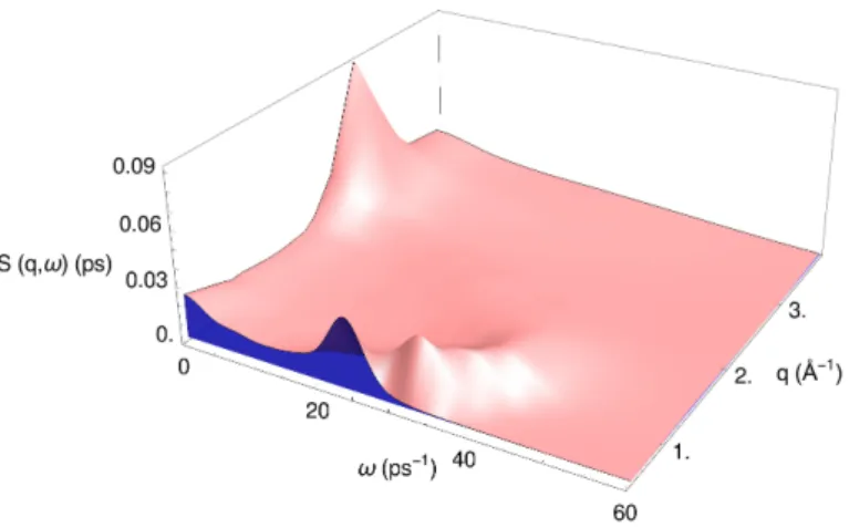
model (circles) and the generalized viscoelastic model (lozenges). . . 92 Figure 6.8 Dynamic structure factors,S(q,ω), of liquid Ti at T=2000 K and severalqvalues. . . 92
Figure 6.9 Dispersion relation for l-Ti at T = 2000 K. Open circles and grey squares: AIMD results from the positions of the inelastic peaks in the S(q,ω)and from the maxima in the spectra of the longitudinal current,CL(q,ω), respectively. Full circles with error bars: IXS experimental data at T= 2020 K, from Saidet al. (Ref. [215] ). The open triangles represent the AIMD results for the HWHM of the inelastic peaks ofS(q,ω)whereas the full triangles with error bars stand for the corresponding IXS experimental data (Ref. [215]). Broken line: linear dispersion with the hydrodynamic sound velocity,cs= 4407 m/s. (Ref. [241]). . . 93 Figure 6.10 The HWHM of the central quasielastic peak of theS(q,ω). Open circles: AIMD results
from the positions of the obtainedS(q,ω). Full circles with error bars: IXS experimental data at T= 2020 K, from Saidet al.(Ref. [215]). . . 94 Figure 6.11 Transverse current correlation function, CT(q,t), at severalq-values for l-Ti atT =
2000K. . . 94 Figure 6.12 Same as before, but forCT(q,ω). . . 94 Figure 6.13 Transverse dispersion relation for liquid Ti atT =2000K. Open circles: AIMD results
from the positions of the peaks in the spectraCT(q,ω). The lozenges with error bars (full circles with error bars) are the positions of the transverse-like inelastic modes in the calculated (experimental) dynamic structure factors,S(q,ω), shown in next Fig. 6.14 95 Figure 6.14 AIMD calculated dynamic structure factorsS(q,w)/S(q)for (top to bottom)q= 0.88,
1.01, 1.24, 1.43 and 1.53 Å−1. The vertical scales are offset for clarity. The arrows point to the locations of the transverse-like excitations . . . 96 Figure 6.15 Total electronic density of states (black line) for bcc Ti (β) and l-Ti at 2000 K. The angular
momentun decomposition of the DOS ins(red dashed line),p(blue dash-dotted line), d(green dashed line). . . 96 Figure 6.16 Static structure factor,S(q), of l-Pd atT =1873K. Full line: AIMD calculations. Open
circles: XD data from Waseda [192]. The inset shows the pair distribution functiong(r). 99 Figure 6.17 Same as the previous figure, but for l-Pt atT =2053K. . . 99 Figure 6.18 Normalized AIMD calculated velocity autocorrelation function of l-Pd, l-Pt and l-Ni near
their respective melting points. The inset represents the corresponding power spectrum Z(ω). . . 100 Figure 6.19 Upper part: Intermediate scattering functions,F(q,t), of l-Pd atT =1873K (full lines)
and l-Pt atT = 2053K (dashed lines) at several values ofq/qp. Lower part: Same as before but for the dynamic structure factors,S(q,ω) . . . 101 Figure 6.20 Longitudinal dispersion relation for l-Pd atT =1873K (circles) and for l-Pt atT =2053
K (diamonds). . . 101 Figure 6.21 AIMD calculated dynamic structure factorsS(q,ω)/S(q)of l-Pd atT =1873K and
sev-eralq-values. The vertical scales are offset for clarity. The arrows point to the locations of the TA modes. . . 102 Figure 6.22 Same as the previous figure, but for l-Pt atT =2053K. . . 102 Figure 6.23 Total electronic DOS (black line) for l-Pd and l-Pt near their respective melting points, as
obtained from the present AIMD calculations. The angular momentum decomposition of the DOS ins(red dashed line) andd(blue dashed line). . . 103 Figure 7.1 S(q)for l-Zn near melting. Full lines: simulation results. The symbols denote
exper-imental measurements, triangles: x-ray data from Ref. [192], circles: x-ray data from Ref. [262], squares: neutron data from Ref. [261]. The inset showsg(r)with the same meaning for lines and symbols. . . 110 Figure 7.2 Detail ofCT(q,t)forq=1.84(full line) and3.71−1(dashed line). The latter has been
List of Figures IX
Figure 7.4 CT(q,ω)for wavevectors shown in the graphs. (a) Belowqp. (b) Aboveqp. (c) Results forq=2.54Å−1; circles: simulation data, lines: fit results and its two components. (d) Same as (c), but forq=3.37Å−1.. . . 112 Figure 7.5 CL(q,ω)for wavevectors shown in the graphs. (a) Belowqp. (b) Aboveqp. (c) Results
forq= 2.07Å−1; circles: simulation data, lines: fit results and its three components. (d) Same as (c), but forq=3.95Å−1. . . 113 Figure 7.6 S(q,ω)for someqvalues in the 1psBZ. . . 114 Figure 7.7 Comparison of IXS measurements atq = 1.06Å−1 and AIMDI(q,E)obtained from
the properly modifiedS(q,ω)(see text) forq=0.96and1.11Å−1.. . . 115 Figure 7.8 Comparison among S(q,ω) (full line), CL(q,ω)(dashed line) and CT(q,ω)
(dash-dotted line), scaled so as to fit in the same graph, for twoqvalues in the 1psBZ. The vertical lines denote the position of the maximum ofCT(q,ω). . . 115 Figure 7.9 Left panel: longitudinal and transverse natural frequencies. Circles: high energy modes.
Triangles: low energy modes. Full symbols: longitudinal modes. Open symbols: trans-verse modes. Right panel: corresponding apparent frequencies. Symbols have the same meaning as in the left panel. . . 116 Figure 7.10 Comparison between AIMD calculatedCT(q,ω), shown by symbols, and MC results,
shown as lines. Theqvalues shown are0.96Å−1(displaced 0.03 units upwards),2.35 Å−1(displaced 0.015 units upwards), and3.28Å−1. The lines are repeated slightly dis-placed above (dashed lines) in order to observe more clearly the double-mode structure where it exists. . . 117 Figure 7.11 Isolines for the weighting functionγ(q,k,p)atq=0.96(a),1.57(b),2.98(c), and4.63
(d) Å−1. The plotted contours correspond to 35 (closest to the diagonal), 50, 100, 150, · · ·, units. . . 118 Figure 7.12 MT(q,t)for the wavevectors shown. Circles: AIMD results. Dashed line: fast part.
Thin solid line: MC component. Thick solid line: total theoretical function. . . 118 Figure 7.13 Comparison between AIMD calculatedCL(q,ω), shown by symbols, and MC results,
shown as lines. Theqvalues shown are1.75Å−1(full line and circles), and2.07Å−1 (dashed line and squares) in the left panel, and3.27Å−1(full line and circles) and4.07 Å−1(dashed line and squares) in the right panel. . . 119 Figure 7.14 Comparison between AIMD calculated S(q,ω), shown by symbols, and MC results,
shown as lines. Theqvalues are shown in the graphs. . . 120 Figure 7.15 Normalized velocity autocorrelation function for l-Zn. Symbols denote the AIMD
re-sults. The full line is the theoretical MC function, with the dashed and dash-dotted lines representing its longitudinal and transverse components, respectively. The inset shows the corresponding power spectra. . . 121 Figure 7.16 Comparison of OF-AIMDI(q,ω)obtained from the properly modifiedS(q,ω)(full line)
and IXS measurements by Hosokawaet al.(open circles) [247] forq=0.66, 0.79, 0.92 and 1.06 Å−1. . . 125 Figure 7.17 OF-AIMD dispersion relations for l-Sn at T=573 K. Black circles:S(q,ω)dispersion. Red
circles:CL(q,ω)dispersion. Blue squares:CT(q,ω)dispersion. The second propagat-ing mode inCT(q,ω)is displayed as filled squares. . . 125 Figure 7.18 Dispersion relations of the maximums using the mDHO model. (a)F(q,t)fit (black
Figure 7.19 a) Dispersion relation of the maximums of each mDHO in theCL(q,ω)(red triangles) and the totalCL(q,ω), which is the sum of both mDHO and the diffusive term (purple stars). (b) Dispersion relation of the natural frequencies of each mDHO inCL(q,ω)(red triangles) andCT(q,ω)(blue squares). Open and closed symbols differentiate between first and second mode. . . 126 Figure 7.20 Solid line: normalized velocity autocorrelation function,Z(t), obtained for l-Sn at T=573
K. The inset represents the power spectrumZ(ω). Dashed and dotted lines represent the longitudinal and transverse components ofZ(t)andZ(ω), respectively. . . 127 Figure 7.21 FT of the longitudinal current correlation functions at different wave vectors. Black
line: results obtained from MC theory. Red dashed curve: results obtained directly from OF-AIMD. . . 128 Figure 7.22 FT of the transverse current correlation functions at different wave vectors. Black line:
results obtained from MC theory. Red dashed curve: results obtained directly from sim-ulation. . . 129 Figure 7.23 First memory function of the transverse current correlation functions at different wave
vectors. Dashed-dotted line: OF-AIMD results. Dotted line: MC component. Dashed line: binary component. Full line: First memory function obtained from theory as the sum of the binary and MC components. . . 129 Figure 8.1 Partial pair distribution functionsgij(r)of the liquid AgxSn1−x alloy atx= 0.27, 0.50,
0.64 and 0.75. Full, dashed and dotted lines correspond togAgAg(r),gSnSn(r)and gAgSn(r), respectively. . . 134 Figure 8.2 Ashcroft-Langreth partial static structure factorsSij(q)of the liquid AgxSn1−xalloy
atx= 0.27, 0.50, 0.64 and 0.75. Full, dashed and dotted lines correspond toSAgAg(q), SSnSn(q)andSAgSn(q), respectively. . . 134 Figure 8.3 Bhatia-Thornton partial static structure factors and total structure factor of the liquid
AgxSn1−xalloy atxAg= 0.27, 0.50, 0.64 and 0.75. Continuous, dashed and dotted lines correspond toSNN(q),SCC(q)andSNC(q), respectively. The thick continuous lines stand for the calculatedST(q), whereas the open circles are the corresponding experi-mental data of Kabanet al. [285] Note thatSNN(q)is indistinguishable fromST(q)in the scale of the graph.. . . 136 Figure 8.4 Normalized self, relative and ideal VACFs for the liquid AgxSn1−x alloy atT = 1273
K andxAg= 0.27, 0.50 and 0.75. Full blue, dashed red, full thick black lines and green circles correspond to Zs
Ag(t), ZsSn(t), ZAgSn(t), andZ0
AgSn(t), respectively. The insets show the comparison between the self-VCFs of the alloy and those of pure liquid Ag (squares) and Sn (triangles) at the same temperature. . . 137 Figure 8.5 Partial intermediate scattering functionsFij(q,t)of the liquid AgxSn1−xalloy at three
List of Figures XI
Figure 8.6 Partial dynamic structure factors Sij(q,ω)of the liquid AgxSn1−x alloy forxAg = 0.27,0.50and0.75. Left pannel: correspondingqmin, namely,0.42Å−1,0.43Å−1,0.45 Å−1forxAg = 0.27,0.50and0.75respectively. Right pannel: q = 1.03Å−1 (xAg = 0.27), q = 1.06 Å−1 (xAg = 0.50) andq = 1.11Å−1 (xAg = 0.75). Circles, red down triangles, blue up triangles and lines correspond toSAgAg(q,ω),SSnSn(q,ω) SAgSn(q,ω)andSNN(q,ω), respectively. The insets show103Sij(q,ω). TheSAgSn(q,ω) for theq-values shown in the right pannel are not displayed because they are negative for allω. . . 141 Figure 8.7 Partial longitudinal current correlation functions,CL
ij(q,ω), for the liquid Ag–Sn alloy atT =1273K and three concentrations. The full, dashed and dot-dashed lines, and the red open circles and blue stars representCL
AgAg(q,ω),CLSnSn(q,ω),CLAgSn(q,ω), CL
NN(q,ω), andCLcc(q,ω)/(xAgxSn)respectively. . . 143 Figure 8.8 Longitudinal dispersion relationsωL
AgAg(q)(red circles),ω L
SnSn(q)(blue squares), andωL
NN(q)(black triangles), for the AgxSn1−xliquid alloy at several concentrations. The continuous and broken lines show the longitudinal dispersion relations of pure liq-uid Ag and Sn atT =1273K, respectively. . . 143 Figure 8.9 AIMD results for the total DOS (full line) of the liquid AgxSn1−x alloy at three
con-centrations. The dotted, dashed and dash-dot lines refer tos,p, anddchannels. For comparison we have also plotted the DOS for pure l-Sn and l-Ag at the same tempera-ture as obtained by the same AIMD method. . . 145 Figure 9.1 Intrinsic and average electronic density profiles for Hg at 300 K. Also shown is the
ex-perimental pair correlation function of the bulk liquid. . . 167 Figure 9.2 Reflectivities for Hg at 300 K. Symbols correspond to experimental data using a hydrogen
atmosphere or in vacuum. Continuous line: AIMD results obtained from the intrinsic profile. Dashed line: AIMD results obtained by depleating by 10% the height of the first layer in the intrinsic profile. . . 167 Figure 9.3 Intrinsic electronic density profiles for Bi and Pb. Also shown are the experimental pair
correlation functions of the bulk liquids. The different functions are shifted vertically for clarity. . . 168 Figure 9.4 Reflectivities for liquid Bi and Pb (multiplied by two for clarity). . . 168 Figure 9.5 Non coulombic part of the local pseudopotential before (full curve) and after (dashed
curve) force-matching. . . 170 Figure 9.6 Difference between thexandzcomponents of the forces as computed with KS-AIMD
simulations [305] and OF-AIMD calculations, before (solid line) and after (dashed line) force-matching. . . 170 Figure 9.7 Transverse pair correlation function for different layers at the free liquid surface ofl-Sn
at T= 600 K and T= 1000 K. Open circles: bulk experimental data of Itamiet al. [269]. Black line: gT(r)calculated at the outmost layer. Red line: gT(r)calculated at the second layer. Green line:gT(r)calculated at the central layer. Insets: distribution of the number of in-plane neighbours for different regions of the slab. . . 172 Figure 9.8 Average ionic DP (full curve, shifted upwards by2.5units) and intrinsic ionic DP (dashed
curve) at T=600 K and 1000 K. At 1000 K the lower full curve corresponds to the intrinsic ionic DP obtained using the simulation data from [305]. . . 173 Figure 9.9 Comparison of the intrinsic electronic density profiles and reflectivities at 600 K (full
line) and 1000 K (dashed line) with the experimental reflectivity (dots) [47].. . . 173 Figure 9.10 S(q,ω)at differentqvalues and depths: bulk region (green curve), second layer (red
curve) and first layer (black curve). . . 174 Figure 9.11 CL(q,ω)at differentqvalues and depths. Same legend as Fig. 9.10 . . . 174 Figure 9.12 FT transverse in XY plane current correlation functions at differentqvalues and depths.
Figure 9.13 FT transverse perpendicular to the surface current correlation functions at differentq values and depths. Same legend as Fig. 9.10. . . 175 Figure 9.14 q-dependent adiabatic sound velocity,cs(q), inl-Sn at 600 K. Black circles: First layer.
Red squares: Second layer. Blue triangles: Bulk region. Filled green diamonds: IXS data for bulk l-Sn at 593 K by Hosokawaet al. [322]. Inset: Dispersion relation of the intermediate scattering function. Open symbols: Results from the fit to the model 175. X: OF-AIMD results from the direct FT. The horizontal arrow atq = 0 stands at the experimental adiabatic sound velocity [324] . . . 176 Figure 9.15 Dispersion relation ofCL(q,ω)at different scattering depths. Open and full symbols:
High and low energy modes respectively. Black circles: First layer. Red squares: Second layer. Blue triangles: Bulk region. Dashed line: theoretical dispersion relation of the capillary waves in the system [323]. . . 177 Figure 9.16 Comparison of dispersion relations forCL(q,ω)in the bulk region of the slab (blue
triangles) and in bulk l-Sn from Chapter 7 (red triangles). . . 177 Figure 9.17 Dispersion relations for CT
p(q,ω) at different depths. Open and full symbols: low
energy and high energy modes, respectively. Black circles: First layer. Red squares: Second layer. Blue triangles: Bulk region. X: OF-AIMD results from the direct FT. . . 178 Figure 9.18 Dispersion relations forCT
z(q,ω)at different depths. Open, dashed and full symbols:
low energy, Lamb wave modes and high energy modes, respectively. Black circles: First layer. Red squares: Second layer. Blue triangles: Bulk region. X: OF-AIMD results from the direct FT. Dashed, dotted and dashed-dotted lines: Lamb waves dispersion relation corresponding to n=4, 5 and 6, respectively. . . 179 Figure 9.19 Comparison of dispersion relations forCT
p(q,ω)in the second layer (red squares) and
theCT(q,ω)in bulk l-Sn from Chapter 7 (green squares). . . 180 Figure 9.20 Comparison of dispersion relations forCT
z(q,ω)in the second layer (red squares) and
the CT(q,ω)in bulk l-Sn from Chapter 7 (green squares). Discontinuous line: dis-persion relation of capillary waves. Continuous and dash-dotted lines: Lamb waves dispersion relation corresponding to n=4 and n=6, respectively. . . 180 Figure 9.21 Scheme representing the combination of twoCL(q,t)not in the XY plane giving rise to
a wave propagating in the XY plane and oscillating perpendicular to the surface.. . . 180 Figure 9.22 Non coulombic part of the local pseudopotential before (black curve) and after (red
curve) force-matching. . . 182 Figure 9.23 Comparison of thezcomponents of the forces as computed with KS-AIMD simulations
(black curve) and OF-AIMD simulation (red curve), before and after force-matching.. . . 182 Figure 9.24 OF-AIMD calculated IDP. Inset: intrinsic surface structure factor from OF-AIMD (black
line) and experimental data [316] (open circles). . . 183 Figure 9.25 Dynamic structure factor after detailed balance condition and experimental convolution,
I(q,ω), at several wave vectors in all the regions studied. Continuous lines: OF-AIMD results. Open circles: IXS experimental results at the smallest possible probing depth, 40 Å [316]. . . 184 Figure 9.26 OF-AIMD dynamic structure factor after detailed balance condition,SQ(q,ω), at
sev-eral wave vectors in all the regions studied.. . . 184 Figure 9.27 CL(q,ω)at different wavevectors and probing depths. . . 185 Figure 9.28 Longitudinal viscosity at different wavelengths and depths. . . 186 Figure 9.29 q-dependent adiabatic sound velocity at different depths in the FLS. Same legend as Fig.
9.28. The horizontal arrow indicates the experimental value at melting [253]. . . 187 Figure A.1 Two-center bipolar coordinates . . . 192 Figure C.1 Non-Coulombic parts of the initial BLPS (for Ga and Li) and local channel of NLPS (for
List of Figures XIII
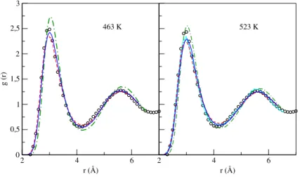
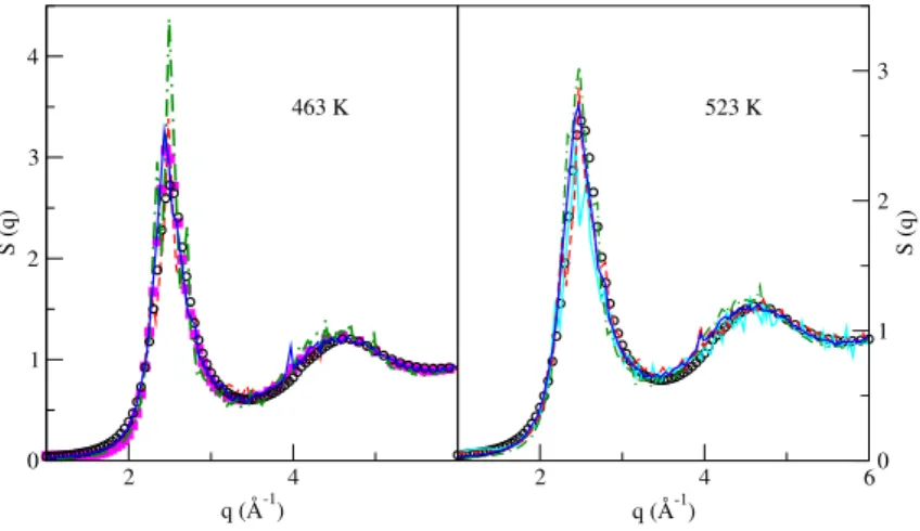
Figure E.1 Static structure factor, S(q), at different temperatures. Full lines: OFDFT results. Red circles: experimental X-ray (XR) results by Waseda [192]. Blue circles: neutron scatter-ing (NS) by Itami [269]. . . 199 Figure E.2 Self diffusion coefficients at different temperatures. Black line: OFDFT results. Full
circles: Experimental results by Brunson and Gerl [294]. Open circles: Experimental results by Ma and Swalin [329]. Full squares: Experimental results under microgravity by Itami et al. [330]. Open squares: AIMD results by Itami et al. [269]. Full triangles: Classical MD (CMD) results by Itami et al. [269]. Open triangles: CMD results by Mouas et al. [331]. . . 200 Figure E.3 Intermediate scattering function,F(q,t), for several q-values at T= 573 K (left) and T=
1273 K (right). Full line: OFDFT results. Dashed line: KSDFT results by Calderín and co-workers [228]. . . 201 Figure E.4 Adiabatic sound velocity,cs, at different temperatures. Full circles: OFDFT results. Full
squares: experimental results from Hosokawa and coworkers [322]. Full triangle: exper-imental result from Blairs [233]. Stars: extrapolated results using experimental equation from [233]. . . 201 Figure E.5 Shear viscosity coefficients at different temperatures. Black line: OFDFT results. Full
L I S T O F T A B L E S
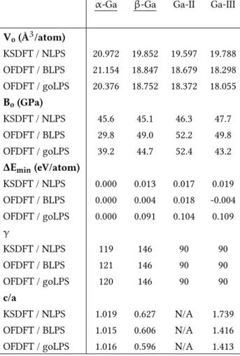
Table 1 Ga bulk crystal properties calculated with the three different methods (KSDFT/NLPS, OFDFT/BLPS, and OFDFT/goLPS): equilibrium volume (V0), bulk modulus (B0), equi-librium total energy relative toα-Ga (∆Emin=Emin−Eα−Ga
min ) for other bulk phases, lattice vector angleγ, and the ratio between two cell lattice vectorsc/a. Underlined solid phases were used as reference data in the goLPS construction. . . 63 Table 2 Li bulk crystal properties calculated with the four different methods (KSDFT/NLPS,
OFDFT/BLPS, KSDFT/PAW and OFDFT/goLPS): equilibrium volume (V0), bulk mod-ulus (B0), equilibrium total energy relative to bcc-Li (∆Emin=Emin−Ebcc−Li
min ) for other bulk phases. Underlined solid phases were used as reference data in the goLPS construction. . . 65 Table 3 Differences between forces (Eq. 154) for the liquid Li configurations used as references,
calculated with KSDFT/PAW and OFDFT along with the BLPS and goLPS. . . 65 Table 4 Differences between forces (Eq. 154) for the liquid Li configurations used to test
trans-ferability, calculated with KSDFT/PAW and OFDFT along with the BLPS and goLPS. . . 66 Table 5 Self-diffusion coefficients of liquid Li in the thermodynamic states studied. . . 68 Table 6 Ca bulk crystal properties calculated with the three different methods (KSDFT/PAW,
OFDFT/LPS, and OFDFT/goLPS): equilibrium volume (V0), bulk modulus (B0), equilib-rium total energy relative to fcc-Ca (∆Emin=Emin−Efcc−Ca
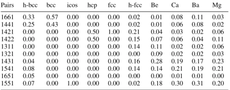
min ) for other bulk phases. Underlined solid phases were used as reference data in the goLPS construction. . . 69 Table 7 Common neighbour analysis of the AIMD configurations of l-Ti at 2000 K compared
with several local structures. . . 88 Table 8 Input data for the different thermodynamic states studied in this work. ρis the total
ionic number density andT is the temperature.Ncis the total number of configurations. 98 Table 9 Comparison between calculated number densities and experimental densities by Waseda
[192,271] at temperatures ranging from 573 K to 1873 K. . . 124 Table 10 Thermodynamic input data of the liquid AgxSn1−x alloy atT = 1273K, used in the
present AIMD simulation study. The total ionic number density,ρ, was taken from Ref. [278]. . . 133 Table 11 Calculated coordination numbersnijand the Warren SRO parameterα1for the liquid
AgxSn1−xalloys at the thermodynamic states given in Table 10. . . 135 Table 12 Diffusion coefficients (in 10−4cm2/s) and parameterγAgSnof the liquid AgxSn1−x
alloy at the thermodynamic states given in Table 10.. . . 138 Table 13 Calculated values of the adiabatic sound velocitycs(in m/s) and the shear viscosityη
(in GPa ps) for the liquid AgxSn1−xalloy at the thermodynamic states given in Table 10. For comparison, we also include the AIMD values obtained for pure liquid Ag and Sn.[228,230] The experimental data were taken from Ref.[297]. . . 144 Table 14 Simulation details.. . . 165 Table 15 Calculation details for each of the thermodynamic states studied. . . 171 Table 16 Comparison of NLPS and BLPS KSDFT-PBE bulk properties of the bcc, fcc, sc, and CD
phases of Li. The bulk modulus (B) is in GPa, the equilibrium volume per atom (V0) is in Å, and the equilibrium total energy (E0) is in eV/atom. All total energies are listed relative to bcc-Li equilibrium total energy. . . 196
1
I N T R O D U C T I O N1.1 t h e s i m u l at i o n o f t h e l i q i d s tat e .
At present, three major research fields can be distinguished in Physics: Particle and High Energy Physics which deal with very small bodies; Cosmology, dealing with the very big; and Non-Linear Physics and Nanophysics, which deal with complex behaviors. This thesis corresponds to this last field in which we will study liquid metals throughab initiosimulation techniques based on Density Functional Theory [1–3].
One of the major difficulties in describing liquid systems, is the lack of ideal models like those of the ideal gas or the harmonic solid which can be exactly solved. Nevertheless, there have been various models which have attempted to describe, in a more or less accurate way, the behavior of liquid systems of diverse nature. An example is thelattice model, in which the similarity between liquids and solids is exploited; or theperturbative model where a similar philosophy to other fields in Physics is followed in the sense that liquid systems are described in terms of perturbations of a reference system whose properties are known.
A different approach for the study of the behavior of liquid systems is through computer simulation techniques; in particular, Molecular Dynamics (MD). In fact, MD methods are an extremely useful tool to investigate the behavior of both macroscopic and low dimension systems since it not only allows to compare the reliability of different theoretical models but also provides information which would be very difficult (or even impossible) to acquire experimentally. The computation power to perform complex calculations, enables to solve the equation of motion of a group of particles in time with an almost total control over the conditions of the system either thermodynamic (pressure, external fields) or microscopic (interactions, composition). In other words, the liquid state can be simulated in a precise way obtaining exact results given the level of approximations used in the simulation.
The first MD study was performed by Alder and Wainwright in 1957 [4]. They studied the solid-liquid phase transitions of a system of particles interacting through a hard-spheres potential,
V(r) =
∞ r6σ
0 r > σ
(1)
Later, in 1959, they published a work where they detail the purpose, methodology, and applications and limi-tations of MD [5]. In 1964, in a study which became a milestone in the development of this technique, Rahman [6] presented a simulation with 864 argon atoms at 94.4 K and a density of 1.374 gcm−3with a Lennard-Jones (LJ) potential:
V(r) =4[(σ/r)12− (σ/r)6]
The final results enabled the calculation of different microscopic correlation functions. For this particular study and his whole career in general, Rahman is considered as one of the pioneers in the application of computational methods for the study of physical problems, and many of the codes used nowadays are inheritors of the ones developed by him in this period. Following this line of work, between 1967 and 1968, Verlet performed simulations of LJ systems calculating different thermodynamic [7] dynamic and structural properties [8], improving technical aspects like the algorithm for propagating the coordinates, which ended up as the Verlet algorithm. A review of the most relevant work performed in the mid 70’s can be found in Ref. [9].
Figure 1.1:Relationship between experimentation, theory and simulation; and how this last one acts as a bridge between the former two [10].
In the 70s, when computational simulation was widely used by the scientific community, a question arose of whether simulation techniques belonged to theory or experimentation. Even though it may seem just a nomi-nal problem, behind it lay important conceptual aspects. The simulated systems are not real but mere numeric calculus used to described a specific case. However, the method shares several points with experiments: simula-tion as well as experiments are prepared, are set to run, data is generated, and these are finally analyzed, while theoretical work follows other paths based on reductionism, mathematical formulae and the prevision of new phenomena. How was this dilemma solved? It is accepted that simulations conform a field of its own, playing a fundamental role connecting theory and experiment, figure1.1.
In the 80s an important step in the simulation methods was taken by including explicitly the electrons in the calculation. Before then, the interaction was modeled by pair potentials whose parameters were adjusted to experimental data. From the first simulations of argon by Rahman and Verlet, where a LJ potential was used, more sophisticated models were introduced to describe very different systems. For example, potentials to describe the interaction in water [11], proteins [12] or liquid metals [13]. However, apart from the success of these type of methods called Classical Molecular Dynamics (CMD), they faced some important limitations (for example, the problem of transferability of the interaction potential), which did not allow a precise general description of the systems able to reproduce the experimental results.
In 1985, Car and Parrinello published a revolutionary work [14] where they described a method which included the electrons in the simulation, creating what is calledab initioMolecular Dynamics (AIMD), or “ first principles” MD. In this method the forces were obtained through calculations of the electronic structure in each step of the generated trajectory in the simulation. Therefore, the interactions were treated in a more fundamental level than CMD. Complex phenomena, like distortion and polarization of the water molecule, as well as bonds being formed [15], emerged from the simulation. As a counterpart, theab initiomethods are much more complex and demanding in computational terms.
1.2 l i q u i d m e ta l s a n d t h e i r a p p l i c at i o n 3
1.2 l i q i d m e ta l s a n d t h e i r a p p l i c at i o n
Liquid metals are a great example of systems which combine a relevance both in industrial applications and basic science. Research in liquid metals has increased in recent years due to their numerous applications in diverse fields: fusion energy, as plasma facing components [18]; medicine, for tumor therapy, bone disease repair and nerve connections [20]; nanoelectronics, for low dimension circuits [21]; and soft robotics, for wearable technology [22].
Fusion energy could be the solution to many energetic and environmental challenges being faced today by human kind. That is why many research is focused in developing the technology required to maintain plasma at such high temperature without destroying the machinery containing it. Liquid metals have become a promising plasma facing component because their properties will not be modified by the displacement of atoms by their collision with particles escaping from plasma. Moreover, they can withstand the high temperatures inside the fusion reactor. The most favorable materials are liquid lithium (Li) and liquid tin (Sn). Some experiments have already been carried out to study their performance at high temperatures. However, computer simulations would be of great help in understanding the properties and behavior at different situations.
For biomedical applications, all the compounds must have specific thermal and electrical properties, fluidic features, plasticity, chemical stability, mechanical performance, biocompatibility and low cost. Promising candi-dates for alloying are: gallium (Ga), indium (In), Sn, bismuth (Bi), cadmium (Cd), and zinc (Zn). All these elements can be potentially described with computer simulations, as well as their liquid binary and ternary alloys.
On the other hand, liquid metals, in particular the monatomic, have been recognized for many years as the prototype of simple liquids, since they englobe most of the physical properties of real fluids without the com-plications that can be present in each system in particular [23]. MD simulations with realistic ionic potentials are a very useful tool for the investigation of liquids at a microscopic level since they provide information on the atomic trajectories which complement the information obtained from experiments, providing access to some dynamic properties which are very difficult (or even impossible) to obtain experimentally.
2
T H E O R Y O F S I M P L E L I Q U I D S : A N I N T R O D U C T I O N 2.1 s tat i s t i c a l m e c h a n i c sThis section is devoted to a brief summary of the principles of classical mechanics and to the discussion of the connection between statistical mechanics and thermodynamics. Consider an isolated, macroscopic system consisting ofNidentical particles, each of which has three translational degrees of freedom. The dynamical state of the system at a given time is completely identified by the3Ncoordinates,~ri, and3Nmomenta,~pi, of the particles. The values of these variables define aphase point,ξ, in a6N-dimensionalphase space,Γ,
Γ ≡{~ri(t),~pi(t)} , i=1...N (2)
andξ = (~r1,~p1, ...,~rN,~pN). The evolution of the phase point will describe a curve orphase trajectory in the phase space,ξ(t), determined by Hamilton’s equations,
∂~ri
∂t = −
∂H ∂~pi
, ∂~pi
∂t =
∂H ∂~ri
(3)
whereH=H(~ri,~pi;t)is the Hamiltonian of the system. In principle, the trajectory could be calculated directly from equation3, but in a thermodynamic system the dimension ofΓ is of the order of the Avogadro’s number, making the task impossible. Therefore, a statistical treatment is necessary.
The aim of equilibrium statistical mechanics is to calculate observable properties of the system either as aver-ages over a phase-space trajectory or as averaver-ages over an ensemble of systems, each of which is a replica of the system of interest. An ensemble is an arbitrarily large collection of imaginary systems, all of which are replicas of the system of interest insofar as they are characterized by the same macroscopic parameters. The systems of the ensemble differ from each other in the assignment of the coordinates and momenta of the particles, and the ensemble is represented by a cloud of phase points whose distribution is described by a phase-space probabil-ity densprobabil-ityf(Γ) =f(~ri,~pi;t). The quantityf(ξ)dΓ is the probability that at timetthe physical system is in a microscopic state represented by the phase pointξinside the volumedΓ, representing,
dΓ =
N Y
i=1
d~rid~pi (4)
The probability densityf(Γ)must be normalized, meaning its integral over the entire phase space must be unity. Given a complete knowledge of the probability density, it would be possible to calculate the average value of any function of the coordinates and momenta. The explicit form of the equilibrium probability density depends on the macroscopic parameters chosen to characterize the ensemble. A particularly simple case is one where the systems of the ensemble are assumed to have the same number of particles, same volume and same total energy. An ensemble constructed this way is calledmicrocanonicalensemble. When the temperature is kept constant instead of the total energy, the ensemble is calledcanonical.
Thermodynamic properties of a system, with some exceptions, can be represented as averages of certain func-tions of the coordinates and momenta of the constituent particles called dynamic variables,A(~ri,~pi). These dynamic variables can be averaged over the ensemble to obtain the associated thermodynamic property,hAi,
hAi= Z
Γ
dΓ f(~ri,~pi)A(~ri,~pi) (5)
Another alternative to calculate the statistical average ofA(~ri,~pi)is as a time average over the dynamical evolution through the phase space. After a suitable lapse of time the system will have sampled the spaceΓ accordingly to the conditions imposed by the force field, and its mean value will be given by,
¯
A= lim
T→∞ 1 T
ZT
0
dtA(~ri,~pi;t) (6)
It is reasonable to suppose that the phase trajectory of the system will pass more frequently through phase points with a higher probability while those with a zero probability will never be visited. Therefore, for reasonable long times, the trajectory ofA(t)will have sampled the entire ensemble, and the ensemble average and time average will coincide,
hAi=A¯ (7)
This result, introduced by Boltzmann, is known as theergodic hypothesis, and is essential for the development of MD.
2.2 t i m e - c o r r e l at i o n f u n c t i o n s
In a thermodynamic system in equilibrium, the value of a dynamic variableA(t)will be constant1. However, if the scale is reduced so is the statistics over which the study is made, andA(t)starts to fluctuate around its mean value. These microscopic spontaneous fluctuations which move away the system from its equilibrium state conform the main object in the description of the dynamical properties of the system [24,25].
A crucial aspect about these fluctuations in the system comes through thefluctuation-dissipation theorem, which indicates that the laws and mechanisms describing the behavior of the fluctuations are the same as those that manifest in the system’s response to an external perturbation. The connection between these different aspects is enormously meaningful: on one hand, it establishes the possibility to analyze the behavior of a system in a non-equilibrium state from the information obtained from equilibrium; moreover, it connects directly with the experiment, whose methodology consist in analyzing the reaction of a system to perturbations at certain conditions.
The fluctuations of a given space-time variableA(~r,t)are treated through thecorrelation functions. These magnitudes are defined as the statistical average of the product of the dynamic variable in two different space-time points:
CA(~r1,t1,~r2,t2)≡ hA(~r1,t1)A(~r2,t2)i (8)
where h. . .i stands for the ensemble average. CA is an autocorrelation function; a correlation function can connect, in general, two different dynamic variables. Some of their main properties are:
• If the system is in equilibrium, the behavior ofCAcannot depend on the choice of the time origin, therefore:
CA(t1,t2) =CA(t1+τ,t2+τ) (9)
With the choiceτ= −t2the time dependency simplifies:
CA(t1−t2) =hA(t1−t2)A(0)i (10)
If the system is homogeneous and isotropic,CAwill only depend on the distance between points,|~r1−~r2|:
CA(|~r1−~r2|) =hA(|~r1−~r2|)A(0)i (11)
2.3 f u n d a m e n ta l p r o p e r t i e s 7
• Applying Schwartz’s inequality, the time correlation function has an upper limit of its initial values:
CA=hA(t)A(0)i6 p
hA(t)A(t)ihA(0)A(0)i=
=hA(0)A(0)i=CA(0)
(12)
The normalization ofCA(t)is performed by its initial value.
• For long times,A(t)will be completely uncorrelated to its initial valueA(0):
CA t→∞
−−−→ hA(0)i2 (13)
• To study time fluctuations, it is more appropriate that the value taking part in the correlations is the fluc-tuation itself with respect to the mean value:
δA(t) =A(t) −hAi (14)
Therefore, the correlation function decays, in a more proper way, to zero.
• Transforming againδA→Afollowing the previous definition, the spectrum of the time correlation func-tion can be defined,CA(ω), through the Fourier Transform (FT):
CA(ω) = 1
2π Z+∞
−∞
dteiωtCA(t) (15)
Many experimental techniques, as neutron scattering (NS), inelastic neutron scattering (INS) or X-Ray scattering (XRS), consist of spectroscopic readings, or spectrum measurements likeCA(ω).
• It is useful to consider the transformation between position and time spaces:
CA(q) = Z
d~re−i~q·~rCA(r) (16)
Working inrspace the spatial correlations are analyzed directly (distances, angles); however,qspace is more appropriate for the study of collective phenomenons and for comparison with actually measured quantities.
2.3 f u n d a m e n ta l p r o p e r t i e s
The main dynamic variables in the study of the thermal movement are the number density, defined as:
ρ(~r,t) =
N X
i=1
δ(~r−~Ri(t)) (17)
whereδ(~r)represents the Dirac delta and~Ri(t)is the position of thei-th particle, and the density current due to the overall motion of the particles:
~J(~r,t) =
N X
i=1
~vi(t)δ(~r−~Ri(t)) (18)
2.3.1 Structural properties
The interaction among particles in a liquid system produces correlations between its positions making their space distribution neither perfectly homogeneous nor purely disordered, but characteristic of the peculiarities of their interactions. Theradial distribution function,g(~r), takes into account the spatial correlations appearing in a real system due to the interaction potential. In particular,ρg(~r)is the probability density of finding a particle at a certain distancerfrom a particle at the origin. In a simulation, it is calculated from the distance of each atom of the system to all its neighbours. An histogram is made from the results, in such a way that the integration ofρg(~r)in a sphere of any radius results in the same number of neighbours as an atom has inside that sphere. g(~r)can be understood as a function which adjusts locally the numeric density. In isotropic systems the radial dependency is simplified:g(~r) =g(r).
The general shape ofg(r)for a dense monatomic liquid shows some distinctive characteristics. At smallrit is almost zero due to the high energies required to force atoms to overlap. Theg(r)shows a pronounced peak atr= rmaxwhich is close to the atomic diameter and is identified as the nearest neighbour distance; moreover it also characterizes the sphere of nearest neighbours. Beyond this region, the presence of several oscillations indicates that the average arrangement of particles around an arbitrary atom proceeds through ’clusters’ resembling the shells of neighbours occurring in a crystal. The analogy is however incomplete, both because of the inherent isotropy of the liquid and for the ill-defined character of the shells, which are considerably broader than those of a crystal at finite temperatures. These oscillations decrease in amplitude with increasingr, and eventuallyg(r) approaches the (unit) mean density of the system and the system effectively behaves as a structureless continuum.
The radial distribution function is defined through the following averages:
ρg(~r) = 1
N
*X
i6=j
δ(~r−~Rij) +
, ρ2g(~r−~s) =
*X
i
δ(~r−~Ri) X
j6=i
δ(~s−~Rj) +
(19)
where Nis the number of atoms and~Rij = ~Ri−~Rj. For systems interacting through a pair potential, ther-modynamic quantities like temperature or pressure are accessible from the potential and the radial distribution function [26].
We denote the FT ofρ(~r)asρ(q), namely,
ρ(~q) =
N X
j=1
e−i~q·~Rj (20)
Note, however, thathρ(~r)i= ρ, which is not zero, and therefore, in the same spirit as discussed in equation 14, it is advantageous to consider the fluctuations around this average value, i.e.,
δρ(~r) =ρ(~r) −ρ , δρ(q~) =ρ(~q) − (2π)3ρδ(~q) (21)
An experimentally accessible quantity which is closely related tog(r)is thestatic structure factordefined by,
S(~q) = 1
2.3 f u n d a m e n ta l p r o p e r t i e s 9
S(q)can be determined from NS and XRS experiments. It is connected tog(r)through the FT:
S(~q) = 1
Nhδρ(~q)δρ(−~q)i=
= 1 N * X j
e−i~q·~Rj− (2π)3ρδ(~q)
X
l
ei~q·~Rl− (2π)3ρδ(~q) !+
=
= 1+ 1
N
*
X
j
e−i~q·~Rj− (2π)3ρδ(~q)
X
l6=j
ei~q·~Rl− (2π)3ρδ(~q)
+
=
= 1+ 1
N *Z
d~re−i~q·~r
X
j
δ(~r−~Rj) −ρ
Z
d~sei~q·~s
X
l6=j
δ(~s−~Rl) −ρ
+
=
= 1+ 1
N Z
d~r Z
d~se−i~q·(~r−~s)
*
X
j
δ(~r−~Rj) −ρ
X
l6=j
δ(~s−~Rl) −ρ
+
=
= 1+ 1
N Z
d~r Z
d~se−i~q·(~r−~s)hρ2g(~r−~s) −ρ2−ρ2+ρ2i=
= 1+ρ Z
d~te−i~q·~tg(~t) −1 (23)
The difference between usingρ(~q)or the correctδρ(~q)in the calculation ofS(~q)only affects the value atq=0. This is important from a theoretical point of view, makingS(0)finite and moreover related to thermodynamic quantities as mentioned below. However, from a computational point of view from MD simulations, the value q= 0is never attainable, and therefore it is safe to computeS(q)ashρ(~q)ρ(−~q)i/N. For this reason, in the following we will not make distinctions bewteen the dynamic magnitudes and their corresponding fluctuations in the definitions of the correlation functions.
In isotropic systems,S(~q) =S(q), and the previous integral turns out to be:
S(q) =1+4πρ Z∞
0
drr2[g(r) −1]sinqr
qr (24)
Broadly speaking, the shapes ofS(q)andg(r)in typical simple liquids are remarkably similar, although of course the physical meaning to be attributed to the various features is completely different in the wave vector domain. Thus, the first sharp peak ofS(q)reflects the existence of a dominant nearly regular arrangement of the particles in real space at valueqpeak≈ 2π
rmax. The sharp decrease ofg(r)at small distances is responsible for the subsequent maxima and minima ofS(q), which become more and more damped asqincreases. Eventually, at large wave vectors,S(q)probes the ’hard core’ region whereg(r)is vanishingly small: here the contribution of the integral in equation24becomes negligible, andS(q)→1. In the opposite extreme,S(q→0)reflects in an average sense the features ofg(r), including its asymptotic approach to unity at very large separations. As a consequence,S(0)can be expected to be associated with some macroscopic property of the system. It can be shown [26],
lim
q→0S(q) =ρkBT κT
(25)
whereκT is the isothermal compressibility. The very low values ofS(q → 0)are typical for all liquids near melting, and reflect our very limited ability to compress such systems. This situation is to be compared with those taking place in an ideal gas (whereg(r)≡1for allr, makingS(q) =1at anyq) and in a fluid near the liquid-gas critical point (where the onset of huge density fluctuations over macroscopic distances causesS(0)to diverge).
2.3.2 Dynamic properties
Single particle
The main dynamic quantity used to study the diffusion of the particles in the liquid is thevelocity autocorrelation function,Z(t), defined as,
Z(t) = 1
3h~vi(t)·~vi(0)i (26)
where~vi(t)is the velocity of thei-th particle.Z(t)is a measure of the projection of the particle velocity at time tonto its initial value, averaged over all initial conditions.
The value ofZ(t)att=0can be derived from the equipartition theorem,
Z(0) = kBT
m (27)
For times long compared with any microscopic relaxation times, the initial and final velocities are expected to be completely decorrelated, so thatZ(t → ∞) = 0. Z(t)also has a slowly decaying part and the detailed behavior depends on both density and temperature. In a low density system,Z(t)will decay slowly because the particles will collide with a low frequency. However, if the density is high, the autocorrelation can even take negative values, decaying in damped oscillations. This phenomenon is called’cage effect’, and represents the fact that the particles are surrounded by neighbours and their movement will consist in a number of collisions inside this cage.
There exists a general relationship between the self-diffusion coefficient,D, and the time integral ofZ(t). Consider a set of identical, tagged particles having positions around a point~r(0). If the particles diffuse in time tto positions around~r(t), the self-diffusion coefficient is given by a well-known relation due to Einstein,
D= lim
t→∞ 1 6t
D
|~r(t) −~r(0)|2E (28)
This result is a direct consequence of Fick’s law of diffusion. It is also a relation typical of a stochastic “random-walk” for which the mean-square displacement of the walker becomes a linear function of time after a sufficiently large number of random displacements have occurred. The connection between|~r(t) −~r(0)|2, the mean square displacement, andZ(t)is,
D
|~r(t) −~r(0)|2E= Zt
0 dt1
Zt
0
dt2h~v(t2)·~v(t1)i=
=3 Zt
0 dt1
Zt
0
dt2Z(t2−t1) =6 Zt
0 dt1
Zt−t1
0
dt2Z(t2−t1) =
=6 Zt
0 dτ
Zt−τ
0
dt1Z(τ) =6 Zt
0
dτ(t−τ)Z(τ)
(29)
where the properties of symmetry with respect to time inversion and invariance under time translation have been used. It can be finally shown that,
D=
Z∞
0
Z(t)dt (30)
This equation is an example of an important class of relations, often called “Green-Kubo formula”, whereby a macroscopic, phenomenological transport coefficient is written as the time integral of a microscopic time-correlation function.
2.3 f u n d a m e n ta l p r o p e r t i e s 11
The typical time dependence of the mean square displacement at very short times displays a parabolic increase associated with free-particle behavior. After the initial parabolic behavior, the bulk of the results are consistent with the linear time dependence typical of the diffusive regime.
Collective dynamics
The collective dynamics is studied through the time correlation function associated with the dynamics ofq -dependent density fluctuations defined by theintermediate scattering function,F(~q,t):
F(~q,t) = 1
Nhρ(~q,t)ρ(−~q,0)i= 1 N
*XN
j=1 N X
l=1
e−i~q·(~Rj(t)−~Rl(0)) +
(31)
This function describes the time dependency of the density fluctuations at different length scales. As with the static properties, if the system is homogeneous and isotropic, the vector dependency in~qis reduced to the modulus,F(q,t). The static structure factor is obtained asF(q,0) =S(q).
We may FTF(q,t)back to the space domain to obtain thevan Hove correlation function,
G(r,t) = 1 (2π)3
Z
d~qei~q·~rF(q,t) = 1
N *XN
j=1 N X
l=1
δ(~r+~Rl(0) −~Rj(t)) +
(32)
which is proportional to the probability of finding a particle at(~r,t)given that att=0there is a particle at the origin. It can be split into a ’self ’-contribution withj=lwhich accounts for the single-particle properties, and a ’distinct’ part withj6=lresponsible for collective properties. This separation also appears in theF(q,t).Fs(q,t)
describes the evolution of the correlations where only one particle takes part.
Alternatively, fromF(q,t)we may proceed with a time FT into the frequency domain to obtain thedynamic structure factor,S(q,ω):
S(q,ω) = 1
2π Z+∞
−∞
dtF(q,t)eiωt (33)
As with the static structure factor, it can be measured directly through INS or XRS, being proportional to the differential cross section. In the case of INS, the double-differential cross section takes the form,
d2σ
dΩdω =
qf qi
h
b2cohS(~q,ω) +b2incS(~q,ω)i (34)
whereqiandqfare the incident and scattered wavevectors, andbcohandbincare the coherent and incoherent scattering lengths of the nuclei conforming the system. The incoherent term appears when nuclei with spin different from zero are studied. In the case of inelastic X-ray scattering (IXS) which acts as a coherent probe only, the double-differential cross section takes the form,
d2σ
dΩdω =
e2 mec2
qf qi
(if)1/2|f(q)|2S(q,ω) (35)
whereiandfrepresent the polarization of the incident and scattered photons; andf(q)is the atomic form factor2. Moreover, now the dynamic structure factor has a coherent part only.
One of the most interesting phenomena to study in liquid state dynamics is the existence of propagating modes in the system. These propagating modes represent collective fluctuations that travel in an analogous way as the phonon in a solid. A maximum inS(q,ω)atω6=0is proof of the existence of these type of propagating modes
in the liquid. However, these peaks are difficult to observe in experimental measurements, and their calculation through simulations can also be challenging. In fact, there is not yet a theory correctly describing the behavior of these modes outside the hydrodynamic regime (q →0). Therefore, is not possible to know beforehand if a system can support these modes or not and, if so, in which frequency range.
Another important dynamic variable is the particle current due to the overall motion of the particles,~J(~r,t), previously defined in equation18, and its FT,
~J(~q,t) =
N X
j=1
~vj(t)e−i~q·
~
Rj(t) (36)
which is split into a longitudinal component,~JL(~q,t), and a transverse component,~JT(~q,t), to the wave vector
~
q. Thelongitudinal and transverse current correlation functionsare defined as the autocorrelation functions of the respective components of the current,
CL(q,t) = 1
Nh~JL(~q,0)·~JL(~q,t)i (37)
CT(q,t) = 1 2Nh
~J
T(~q,0)·~JT(~q,t)i (38)
Their respective spectra in the frequency domain are defined asCL(q,ω)andCT(q,ω). The spectrum of the longitudinal current correlation function is directly related to the spectrum of the dynamic structure factor through the relation
q2CL(q,ω) =ω2S(q,ω) (39)
From these relations it can be deduced that both correlation functions contain in essence the same information; however, it is interesting to analyze both.
The transverse current correlation function,CT(q,t), is not associated with any measurable quantity and can only be determined by means of computer simulations. It provides information on the shear modes and its shape evolves from a Gaussian, in bothqand t, at the free-particle (q → ∞) limit, towards a Gaussian inqand an exponential intat the hydrodynamic limit (q→0), i.e.
CT(q→0,t) = 1 βme
−q2η|t|/mρ (40)
whereηis the shear viscosity coefficient,β= (kBT)−1is the inverse of the temperature times the Boltzmann constant andmis the atomic mass. Whereas at both limits the correspondingCT(q,t)take positive values for all times, at intermediateq-values it may show a more complicated behavior, including well defined oscillations within a limited q-range. It is established that liquids, from the macroscopic point of view, cannot support shear waves as solids do. From the atomic scale, this means that transverse current fluctuations will vanish through diffusive processes. This situation is not so when deformations in the wave length and frequencies of the microscopic scale are considered. In this case, the system can sustain transverse modes. Their existence is revealed through side peaks inCT(q,ω). From the calculatedCT(q,t), the shear viscosity of the liquid,η, can be obtained.
Using Mori-Zwanzig’s formalism, which will be introduced in the next chapter, a generalized shear viscosity coefficient,η(q,z), can be defined in terms ofMT(q,t)which is the first-order memory function ofCT(q,t), namely
˜
CT(q,z) = 1 βm
z+M˜(q,z)−1≡ 1
βm
z+ q
2
mρη˜(q,z) −1
(41)
whereC˜T(q,z)andM˜ (q,z)are the Laplace transforms ofCT(q,t)andM(q,t)respectively.
2.4 e x t e n s i o n t o b i n a r y s y s t e m s 13
2.4 e x t e n s i o n t o b i n a r y s y s t e m s
2.4.1 Structural properties
In Chapter8of this thesis, it will be necessary to generalize the previously given expressions for the distribution and correlation functions. In general, the correlation functions will present double subscripts, each one related to each of the species in the alloy. In this way, it will describe the correlation among particles of the same type and between atoms of different types. For example, three partial distribution functions can be defined, gij(r), describing the surrounding of particles of typejaround one of typei. From these functions we can study the local structure of the alloy. From the knowledge ofgij(r), the distribution of nearest neighbours (NNs) can readily be obtained. Ifnijdenote the number ofj-type particles around ani-type particle within a sphere of radiusRij, then
nij=4πρ xj ZRij
0
r2gij(r)dr, (42)
where xj is the concentration of thej-type particles and Rij can be identified with the position of the first minimum of the corresponding radial distribution functionG(r) = 4πr2gij(r)[28]. A way of quantifying the aforementioned ordering tendencies is provided by the Wagner [27] short range order (SRO) parameter for the first neighbour shell,α1, which is defined as
α1=1−
nij xj(xinj+xjni)
(j6=i=1,2), (43)
wherexjis the concentration of thej-type particles,ni =nii+nij(i,j= 1, 2) andnijis the number ofj-type particles around ani-type which are located within a sphere of radiusRij. A positive value ofα1indicates that the liquid presents an homocoordinating tendency, i.e. particles of the same type tend to be surrounded by atoms of their same type. On the other hand, a negative value ofα1indicates the contrary, i.e. a tendency towards heterocoordination. For a random distribution of atoms,α1=0.
Several types of static structure factors are used in the literature to study alloys.
Ashcroft-Langreth
The Ashcroft-Langreth (AL) partial static structure factors are the ones directly describing the different correla-tions between the particles [32].
Sij(q) =δij+4πρ
√
xixj Z∞
0
drr2sinqr
qr [gij(r) −1] (44)
Bathia-Thornton
The Bhatia-Thornton (BT) partial structure factors [24,31] are ideally suited for investigating chemical and topo-logical ordering tendencies in a binary liquid alloy. These are the concentration-concentration, SCC(q), the number-number,SNN(q), and the number-concentration,SNC(q), partial structure factors, and they can be ob-tained from the above AL partial structure factors. Their long-wavelength limits provide microscopic information on the ordering tendencies of the liquid alloy, speciallySCC(q→0).
NN: Number-number.Describes the global structure of the alloy without specifying the type of each particle.
Mathematically it is the static correlation function of the number density in the Fourier space:ρ(q) =ρ1(q) + ρ2(q).
CC: Concentration-concentration. Describes how the particles distribute and gather attending to their chemical species. The correlation function taking part here is the fluctuations’ concentration:∆x(q) = (V/N)[x2ρ1(q) − x1ρ2(q)],
SCC(q) =x1x2[x2S11(q) +x1S22(q) −2(x1x2)1/2S12(q)] (46)
As with equation 25, in the limitq → 0 the static structure factors can be related to thermodynamic in-formation. In particular, SCC(0)takes a value equal tox1x2 if we have an ideal alloy, while deviations from this value indicate the tendency of the system: homocoordinating, if it tends to form pairs of same particles (SCC(q)> x1x2)or heterocoordination, if it tends to form pairs of different particles(SCC(q)< x1x2).
NC: Number-concentration.Describes the cross correlation between density fluctuations and density
con-centration,
SNC(q) =x1x2 h
S11(q) −S22(q) + (x2−x1)S12(q)/(x1x2)1/2 i
(47)
In an ideal alloy there is no such correlation andSNC(q) =0.
Total static structure factor
From the partial AL static structure factorsSij(q), the total neutron weighted static structure factorST(q)is readily evaluated using the expression
hb2iS(TINS)(q) =
2 X
i=1
hb2ii−hbii2
xi+ 2 X
i,j=1
(xixj)1/2hbiihbjiSij(q) (48)
wherehbiiis the coherent scattering length,4πhb2
iiis the total scattering cross-section andhb2i= P2
i=1xihb2ii is the average cross-section per atom. In the case of IXS, the total static structure factor only presents the coherent term, namely,
S(TIXS)(q) =
2 X
i,j=1
(xixj)1/2
fi(q)fj(q)
hf2(q)i Sij(q) (49)
wherefi(q)are the atomic scattering form factors andhf2(q)i=P2
i=1xif2i(q).
AsST(q)is a weighted sum of the partial static structure factors, the experimental determination of the latter involves three independent measurements with different scattering lengths of theiandjspecies. If this is not possible, a common practice to derive them has been the application of the concentration method, which is based on the assumption that the partial pair distribution functions are independent of the alloy concentration.
The presented formulations to calculate the partial static structure factors contain the same information, given the relationships between them through linear combinations. However, each one is better suited to study different aspects of the alloy’s properties.
2.4.2 Dynamic properties
![Figure 1.1: Relationship between experimentation, theory and simulation; and how this last one acts as a bridge between the former two [ 10 ].](https://thumb-us.123doks.com/thumbv2/123dok_es/6147212.180981/18.892.203.680.111.462/figure-relationship-experimentation-theory-simulation-acts-bridge.webp)